Analytic gas orbits in an arbitrary rotating galactic potential using the linear epicyclic approximation

Abstract

A code, Epic5, has been developed which computes, in the two-dimensional case, the initially circular orbits of guiding centra in an arbitrary axisymmetric potential with an arbitrary, weak perturbing potential in solid body rotation. This perturbing potential is given by its Fourier expansion. The analytic solution solves the linear epicyclic approximation of the equations of motion. To simulate the motion of interstellar matter and to damp the Lindblad resonances, we have in these equations introduced a friction which is proportional to the deviation from circular velocity. The corotation resonance is also damped by a special parameter. The program produces, in just a few seconds, orbital and density maps, as well as line of sight velocity maps for a chosen orientation of the galaxy.

We test Epic5  by comparing its results with previous simulations and observations from the literature, which gives satisfactory agreement. The aim is that this program should be a useful complement to elaborate numerical simulations. Particularly so are its abilities to quickly explore the parameter space, to construct artificial galaxies, and to isolate various single agents important for developing structure of interstellar matter in disc galaxies.

1 Introduction

Since the emergence of high spatial resolution two-dimensional velocity field for galaxies, the interpretation of observed velocity fields has become one of the key concerns of the extragalactic scientific community (e.g., Boulesteix et al. 1987; Adam et al. 1989; Bacon et al. 1992; Bacon et al. 2001; Allington-Smith et al. 1997; Hernandez et al. 2003). Of particular importance is the class of galaxies which host bars and/or spiral arms, as they are estimated to be the most abundant types of galaxies in the local Universe (Loveday, 1996).

The theoretical foundation for understanding the kinematics and dynamics of spiral galaxies has been worked out over the last century. Bertil Lindblad (1963, 1964) conceived a picture of circulation of stars between the spiral arms of a quasi-steady rotating spiral potential. Simultaneously, Lin & Shu (1964) presented their density wave theory approaching the problem from a different theoretical point of view. Subsequently, Shu et al. (1973) and Roberts et al. (1979) derived solutions for the circulation of the interstellar medium through such a spiral potential and predicted large scale galactic shocks along the spiral arms. These processes make bars and/or spiral arms potential actors to redistribute angular momentum which will lead to dramatic effects such as intense star formation, build up of bulges, or onset of nuclear activity. In turn, the host galaxies may undergo dramatic secular evolution on time-scales compared to the galaxy dynamical time (see Kormendy & Kennicutt 2004 for a comprehensive discussion).

Beginning with Holmberg (1941) in the pre-computer era and in the 1950s with electronic computers (e.g. P.O. Lindblad 1960), a large number of simulations of development and evolution of structure in galaxies have been made with a variety of computer codes. These studies have often aimed at establishing the details of the flow of gas in and around bars (eg. Athanassoula 1992), as well as the mechanisms which trigger starbursts and nuclear activity in the centers of galaxies (e.g., Shlosman et al. 1989). However, they often involve extensive computational power leading to relatively long computing times.

Several successful attempts have been carried out in order to deliver analytic solutions for observable parameters for some of the effects involved in the above questions (Sakhibov & Smirnov 1989; Canzian 1993; Wada 1994; Lindblad & Lindblad 1994; Schoenmakers et al. 1997; Wong et al. 2004; Fathi et al. 2005; Byrd et al. 2006; van de Ven & Fathi 2010), though they have all exclusively treated one specific morphological feature in each analytic model. While a linear analysis can be a guide for a physical understanding of complicated numerical results from simulations, in these analytic studies, bars and spiral arms have been accounted for separately, and interpretations have been based on marginalizing the effect of the other features. A notable difference between these results and numerical simulations is that the stepwise integration in a detailed simulation requires appreciable computing times, while for analytical calculations the computing time is negligible.

In this paper, we present an analytic solution within the epicyclic approximation, in which we introduce an arbitrary gravitational potential and a damping coefficient for adequate appearance of the corotation resonance. Our solution has been coded as a development of the program Epic (Lindblad & Lindblad, 1994) which was based on the first order epicyclic approximation. The current code, Epic5, derives the response of interstellar matter, originally in circular orbits, to the gravitational potential in a matter of few seconds, which makes it an efficient code for surveying a large parameter space. In section 2, we present the analytical solution for the epicyclic theory with a generic potential, and we describe our code Epic5. We compare results generated by Epic5  with Wada (1994) in section 3, and in section 4, we demonstrate a standard case of a barred galaxy. In section 5 we compare results obtained by Epic5 with observations and simulations made for the galaxy NGC 1365. Finally, we conclude in section 6.

2 Method

The epicyclic description of nearly circular stellar orbits in a circularly symmetric galaxy was developed by B. Lindblad (1927) in order to theoretically explain the observed velocity ellipsoid in the Milky Way galaxy. Later on, B. Lindblad (1958) introduced a rotating perturbing potential in the theory and pointed out the resonances that carry his name. P.O. Lindblad & P.A.B. Lindblad (1994), as well as Wada (1994), introduced gas dynamical friction in the epicyclic approximation. This form of damping the motions would make the first order approximation valid also over the Lindblad resonances, but still not over the corotation resonance.

The potential we are considering in our problem is:

$$\Phi(r,\theta)=\Phi_{0}(r)+\Phi_{1}(r,\theta)$$ (1)

where ($r,\theta)$ are the polar coordinates in a frame co-rotating with the potential at the pattern speed frequency $\Omega_{\rm p}$. $\Phi_{0}(r)$ is the axisymmetric potential, and $\Phi_{1}(r,\theta)$ is an arbitrary perturbing potential developed as a Fourier series

$$\centering\Phi_{1}(r,\theta)=-\sum_{m=1}^{\rm n}\left[\rm P_{\emph{\rm}c,\emph{m}}(\emph{r})\cos\left(\emph{m}\,\theta\right)+P_{\rm s,\emph{m}}(\emph{r})\sin\left(\emph{m}\,\rm\theta\right)\right]\@add@centering$$ (2)

or

$$\centering\Phi(r,\theta)=\Phi_{0}(r)-\sum_{\emph{m}=1}^{\rm n}\Psi_{\emph{m}}(r)\cos\emph{m}\left(\theta-\vartheta_{\emph{m}}(r)\right)\@add@centering$$ (3)

where

$$\centering\Psi_{\emph{m}}^{2}(r)=\rm P_{\emph{\rm}c,\emph{m}}^{2}+P_{\rm s,\emph{m}}^{2}\,\,\,\,\,\,\,\,\text{ and }\,\,\,\,\,\,\,\,\tan(\emph{m}\vartheta_{\emph{m}})=\rm P_{\emph{\rm}c,\emph{m}}/P_{\rm s,\emph{m}}\@add@centering$$ (4)

We consider small deviations, $\xi$ and $\eta$, from circular motion following the usual notation, where

$$r =r_{0}+\xi$$ (5)

$$\theta =\theta_{0}+(\Omega-\mbox{$\Omega_{\rm p}$})\,t+\frac{1}{r_{0}}\eta$$ (6)

and $\Omega(r_{0})$ is the angular frequency of circular motion. In addition, we introduce a frictional force proportional to the velocity deviation from circular motion with the coefficient $-2\lambda$. As Wada (1994) points out, this is analogous to the Stokes’ formula (eg. Yih, 1979, p. 365) where the drag on a sphere moving slowly in a viscous fluid is proportional to the first power of the velocity. The equations of motion, as derived in appendix A, can then be written as:

$$\centering\ddot{\xi}+2\lambda\dot{\xi}-2\Omega\dot{\eta}-4\Omega A\xi\@add@centering =-\frac{\partial\Phi_{1}}{\partial r}=$$

$$= \sum_{m=1}^{n}\big{[}C_{m}\cos m(\theta-\vartheta_{m})+E_{m}\sin m(\theta-\vartheta_{m})\big{]}$$ (7)

$$\ddot{\eta}+2\Omega\dot{\xi}+2\lambda\dot{\eta}+4\lambda A\xi =-\frac{1}{r}\frac{\partial\Phi_{1}}{\partial\theta}=-\sum_{m=1}^{n}D_{m}\sin m(\theta-\vartheta_{m})$$ (8)

where

$$C_{m}=\frac{d\Psi_{m}}{dr};\,\,\,\,\,\,D_{m}=m\frac{\Psi_{m}}{r};\,\,\,\,\,\,E_{m}=m\Psi_{m}\frac{d\vartheta_{m}}{dr}$$

The solution for the motion of the guiding center will then be:

$$\xi=\sum_{m=1}^{n}\big{[}d_{m}\cos m(\theta-\vartheta_{m})+e_{m}\sin m(\theta-\vartheta_{m})\big{]}$$ (9)

$$\eta=\sum_{m=1}^{n}\big{[}g_{m}\sin m(\theta-\vartheta_{m})+f_{m}\cos m(\theta-\vartheta_{m})\big{]}$$ (10)

where the amplitudes $d_{m}$, $e_{m}$, $g_{m}$ and $f_{m}$ are given in appendix A.

2.1 The code: Epic5

The code Epic5 is an extension of the code developed by Lindblad & Lindblad (1994) and computes the analytic solution (9) and (10), as well as its corresponding density and velocity maps, generated by the arbitrary potential. Epic5 derives the axisymmetric potential, $\Phi_{0}$, from a given rotational velocity curve and the perturbing potential, $\Phi_{1}$, is introduced by its Fourier decomposition, P${}_{\rm c,\emph{m}}$ and P${}_{\rm s,\emph{m}}$ (eq. 2).

In addition to the velocity curve and the parameters of the potential, another free input parameter is a constant pattern speed of the potential, $\Omega_{\rm p}$. The damping coefficient of the frictional force, $\lambda$, which was introduced in the analysis to simulate orbits of interstellar matter, is assumed to have a linear tendency with radius. This linearity is determined by the given values of $\lambda$ at the outer inner Lindblad resonance (oILR) and at the outer Lindblad resonance (OLR) of the system (it is taken at 0 kpc if no ILR is present and if no OLR is present, it is taken at $r_{max}$ in the rotation curve). These two values are also given as input parameters in Epic5. This definition of the damping coefficient, $\lambda$, that allows it to vary along the radius, is desirable since it should depend on the gas density.

As can be seen from eqs. 29-32, the introduction of the friction coefficient $\lambda$ has damped the amplitudes and eliminated the singularities at the Lindblad resonances where $\kappa^{2}-\omega_{m}^{2}=0$. However, the singularity at corotation, $\omega_{m}=0$, remains. As shown by Binney & Tremaine (2008, Ch 3.3.3(b)), the stellar motions close to corotation turn into pendulum like oscillations around the Lagrange equilibrium points $L_{4}$ and $L_{5}$. With increasing distance from corotation, the angular amplitude increases until the orbit reaches the equilibrium points $L_{1}$ and $L_{2}$ and flips into a circumcentral orbit (see Figs. 16 and 26 in P.A.B. Lindblad et al. 1996, hereafter LLA96). In the simulations of LLA96 the points $L_{4}$ and $L_{5}$ represent density minima and $L_{1}$ and $L_{2}$ density maxima along the corotation radius.

Actually, our equations of motion (9) and (10) are no longer valid around corotation because when inserting $\theta$ from eq. (6) into the differential equations (7) and (8) we have assumed $\eta/r_{0}<<(\Omega-\Omega_{p})$ which is not true close to corotation where $\Omega-\Omega_{p}$ approaches zero. We then see from eq. (8) that for small $\xi$, $\dot{\xi}$ and $\dot{\eta}$ we get a pendulum like oscillation in $\eta$, and we should not get a linearized equation.

P.O. Lindblad (1960) has pointed out that a time dependent potential can damp all resonances, including the corotation resonance. For a potential that varies as $e^{\gamma t}$, besides the twisting of the orbits around corotation, $\omega_{m}$ in the denominator of eqs. (29) to (32) is replaced by $\sqrt{(}\omega_{m}^{2}+\gamma^{2})$. In similarity to this, in Epic5 the corotation singularity is avoided by replacing the factor $\omega_{m}$ in the denominator of eqs. (29)-(32) by $\omega_{\epsilon}$, where

$$\frac{1}{\omega_{\varepsilon}}=\frac{\omega_{m}}{\omega_{m}^{2}+\varepsilon_{m}^{2}}$$ (11)

where $\varepsilon_{m}=m\varepsilon$ and $\varepsilon$ is an additional input parameter in the code. As illustrated in Fig. 1, the amplitudes of the motion of the guiding center, growing large and of opposite sign on both sides of corotation, are smoothed and brought to zero at the exact resonance distance. $1/\omega_{\varepsilon}$ reaches a maximum of $1/2\varepsilon_{m}$ at the distance $\omega_{m}=\varepsilon_{m}$ from corotation. This means that the stellar elliptical orbits, trapped around corotation, in our case collapses to circular rotation at the corotation radius. This may not be an entirely inappropriate approximation to the solution in the corotation case.

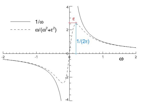
Figure 1: Damping of the amplitudes $\xi$ and $\eta$ at corotation. Solid line: Variation of the amplitudes with $\omega$ according to the first order epicyclic theory with $\varepsilon=0$. Dashed line: Variation of the amplitudes introduced in Epic5.

The derivation of the density is made applying the continuity equation. Using the equation (F-5) in Binney & Tremaine (2008), in our notation the ratio between the perturbed and unperturbed surface densities will be

$$\frac{\rho}{\rho_{0}}=1-\xi-\frac{1}{r}\frac{\partial\eta}{\partial\theta}-\frac{\partial\xi}{\partial r}$$ (12)

where we have assumed the unperturbed surface density $\rho_{0}$ to have a flat distribution.

Epic5 generates a number of supporting plots and diagrams like the rotation curve, the circular frequencies showing the resonances, $\omega$ vs $\kappa$, the perturbing potential, the total potential, radial and tangential perturbing forces, the phase variation of the perturbing potential, orbits, densities, as well as line of sight velocity fields for various position angles of the line of nodes.

The resolution in $r$ required by Epic5 in the tabulated values of the Fourier components of the perturbing potential is related to the increase of the phase shifts $\vartheta_{m}$ with $r$. It is convenient to express this relation in terms of the wavelength of the mode $m=2$ in the spiral structure. If $\lambda_{m}$ is the wavelength of mode $m$, we have approximately for a tightly wound spiral

$$\frac{\rm d\vartheta_{\emph{m}}}{\rm d\emph{r}}=\frac{2\pi}{\emph{m}\lambda_{m}}=\frac{\pi}{\lambda_{2}}$$ (13)

Our requirement for Epic5 to interpret the potential tables $\rm P_{\emph{\rm}c,\emph{m}}(r)$, $\rm P_{\rm s,\emph{m}}(r)$ is $\Delta(m\vartheta_{m})<\pi/2$ or

$$\Delta r<\frac{\lambda_{2}}{2\,n\,}$$ (14)

where $\Delta r$ is the radial increment in the potential table and $n$ is the maximum value of $m$.

Finally, we can choose between counter-clock and clock wise rotation for an easier comparison with observed cases.

3 Epic5 vs Wada’s (1994) model

Wada (1994, hereafter W94) independently provided an analytical model, similar to Epic, representing the behavior of a non-self-gravitating gas in a rotating potential with a weak bar-like distortion. Like the original version of Epic (Lindblad & Lindblad, 1994) there was no solution for the corotation region.

In the model Wada used the Toomre potential for the axisymmetric potential, and for the perturbation the potential given by Sanders (1977)

$$\Phi(R,\psi)=\Phi_{0}(R)(1+\Phi_{\rm b}(R)\cos{2\psi})$$ (15)

$$\Phi_{0}=-\sqrt{\frac{27}{4}}\frac{a\,v^{2}_{\rm max}}{\sqrt{R^{2}+a^{2}}}\;\;\;\;\;\&\;\;\;\;\;\Phi_{\rm b}=\varepsilon_{0}\,a\frac{R^{2}}{(R^{2}+a^{2})^{1.5}}$$ (16)

In these equations, $v_{\rm max}$ is the maximum rotational velocity, $a$ is the core radius and $\varepsilon_{0}$ is a parameter which represents the strength of the bar potential.

We test our code by using the same potential, circular frequency and parameters as W94. W94, however, chooses the friction to be proportional to the velocity in the radial direction only.

W94 considers a core radius, $a$, equal to 1 and a maximum rotational velocity, $v_{\rm max}$, equal to $(4/27)^{1/4}$, simplifying the expressions of $\Phi_{0}$ and $\Phi_{\rm b}$. W94 assumed a weak bar strength, $\varepsilon_{0}$, equal to 0.05 and a pattern speed equal to 0.1.

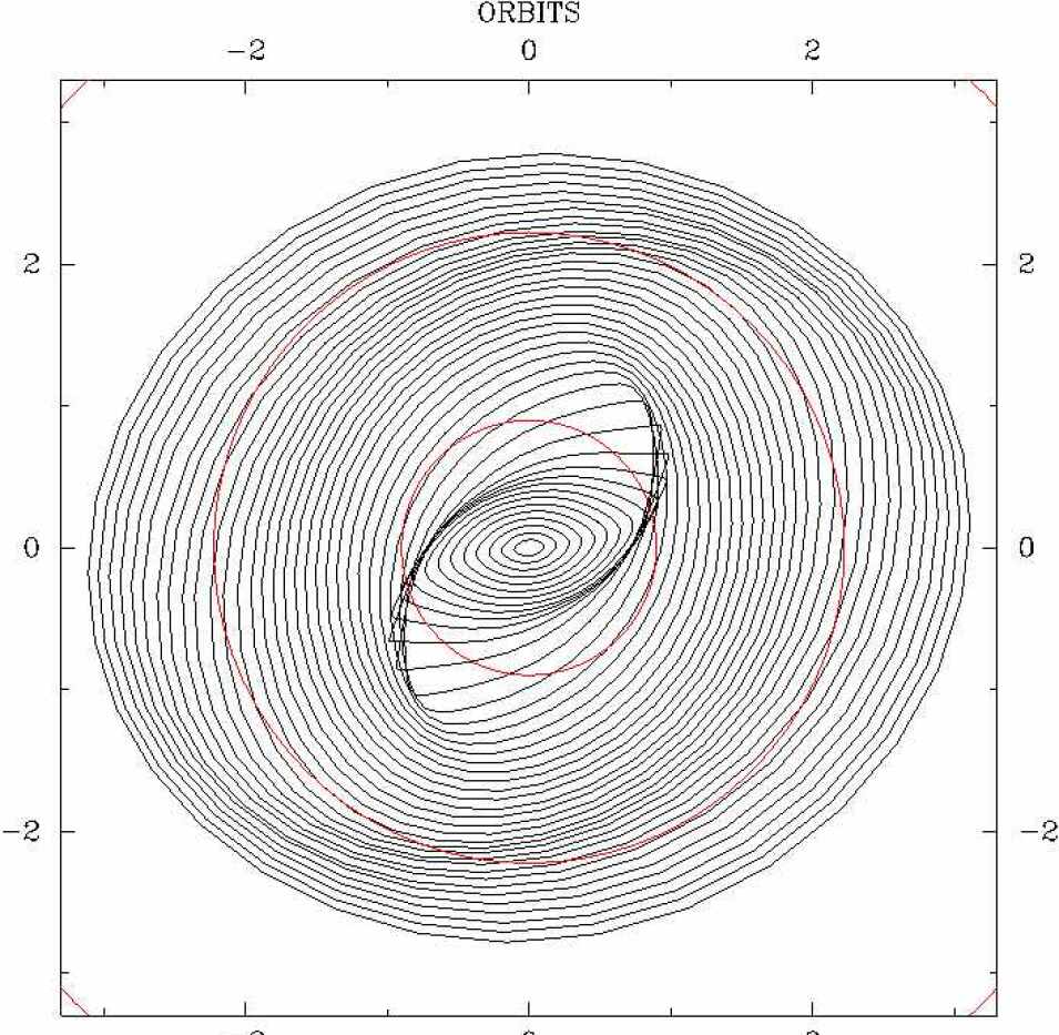
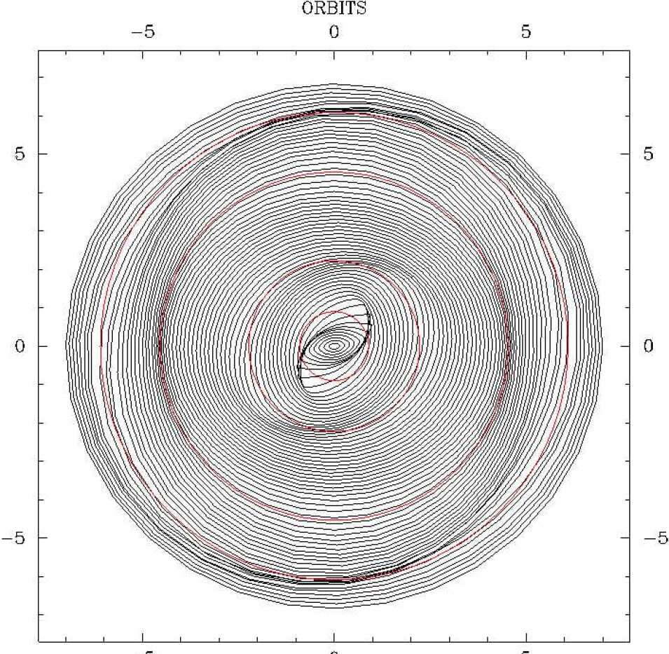
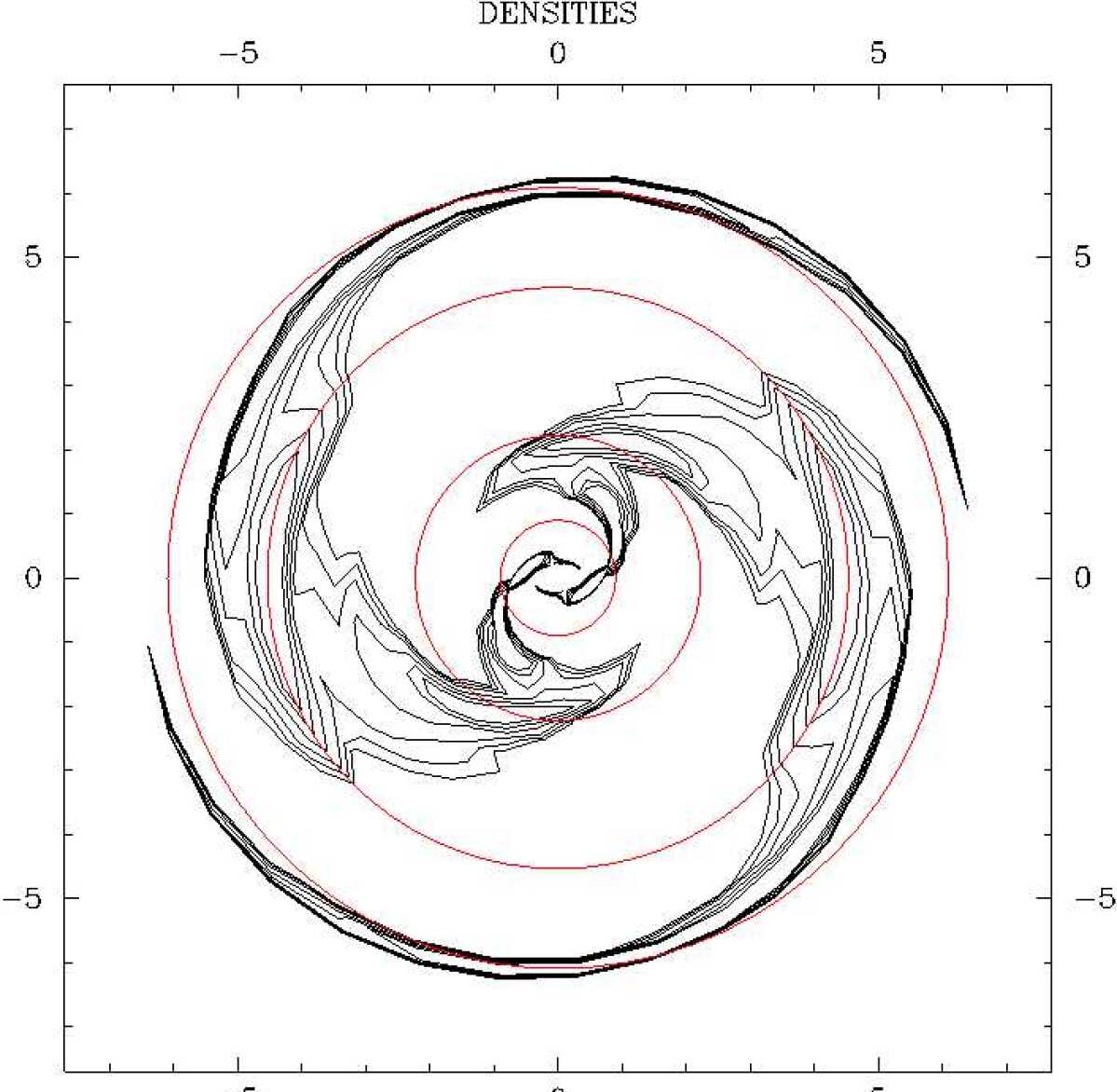
Figure 2: Results from Epic5 for the W94 case. Upper graph: Orbits generated by Epic5 inside corotation. Middle graph: Orbits generated by Epic5 including the outer Lindblad resonance (OLR). Lower graph: Density contours given by Epic5 according to eq. (12). Contours at 1.01, 1.05, 1.1, 1.2, 1.3 and 1.4. Red circles show the positions of resonances iILR, oILR, CR and OLR. The rotation is counter clockwise.

We use in this section the same potentials and derive the input needed for Epic5 from them (the rotational velocity curve and the Fourier components of the perturbed potential). We have also used the same pattern speed of 0.1, a friction coefficient of 0.02 at the oILR and 0.01 at the OLR and a corotation softening coefficient of 0.02. We have located the bar horizontally, equally to its position in W94, and consider a counter-clockwise rotation.

Using these input parameters for our code, we have derived the resonance radia at the same radia as W94: inner/outer Lindblad resonance (iILR and oILR) at 0.90 and 2.22 respectively, corotation (CR) at 4.53 and outer Lindblad resonance (OLR) at 6.09 (see Fig. 1 in W94). We present the orbits generated by Epic5 in the upper panel of Fig. 2, corresponding to the ones presented in Fig. 4 in W94. The leading arms around the iILR and trailing arms around oILR are well presented in both cases. Epic5 damps as well the orbits around corotation, allowing us to present orbits until radia further than CR (see middle panel in Fig. 2).

Epic5 estimates the density map generated by the input potential in the lower panel in Fig. 2, showing the continuation of the spiral arms out to the OLR.

4 Epic5: a demonstration

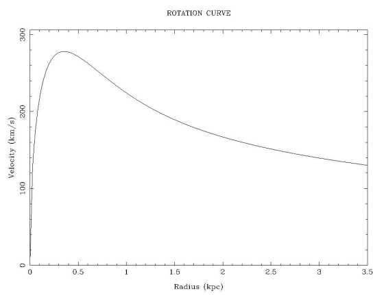
Figure 3: Rotation curve given by two superimposed exponential disks with masses of $11.5\times 10^{9}$ M_⊙ and $2.87\times 10^{9}$ M_⊙ and with scale lengths of 0.194 kpc and 1.15 kpc respectively.

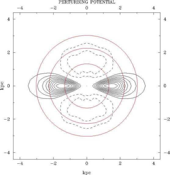
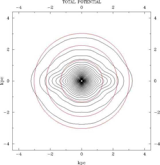
Figure 4: Bar potential. Left graph: Perturbing potential. Dashed lines show the positive contribution and the solid lines the negative contribution. The red circles mark the oILR, corotation and OLR for a pattern angular velocity of 70 km s^-1 kpc^-1. Right graph: Total potential.

We demonstrate in this section a case to illustrate what Epic5 is able to produce. The rotation curve in this case, shown in Fig. 3, is that given by two superimposed exponential disks with masses of $11.5\times 10^{9}$ M_⊙ and $2.87\times 10^{9}$ M_⊙ and with scale lengths of 0.194 kpc and 1.15 kpc respectively (reasonable values for the inner part of barred galaxies, Lindblad et al. 2010). To this, is added an ad hoc perturbing bar potential, described by its Fourier components of cosine of 2, 4, 6, 8 and 10 times $\theta$ for each value of the radius, as seen in Fig. 4 (left graph). This results in the total potential shown in Fig. 4 (right graph). The relative bar strength $|\Phi_{1}|_{\rm min}/|\Phi_{0}|_{\rm min}$ is equal to 0.026.

Fig. 5 shows the variations of $\Omega$, $\Omega\pm\kappa/2$ and $\Omega\pm\kappa/4$ with radius. Our assumed pattern velocity of 70 km s^-1 kpc^-1, which places the oILR close to the minimum of the perturbing potential, is shown as a straight line in the figure, and the resonances are shown by the vertical lines. The iILR lies very close to the center, oILR at 1.33 kpc, CR at 2.26 kpc, and OLR at 3.03 kpc.

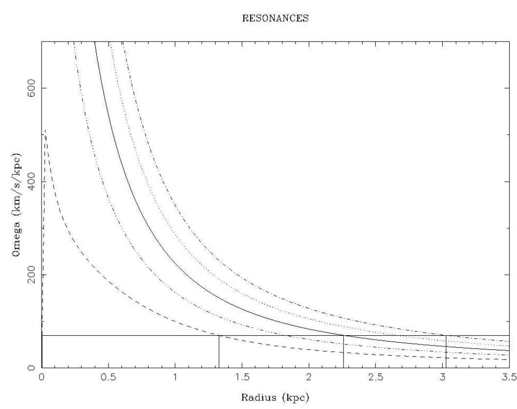
Figure 5: Angular velocity, $\Omega$, against radius derived from the rotation curve (solid line). The dashed line shows $\Omega-\kappa/2$, the dotted-dashed line shows $\Omega+\kappa/2$, the dotted and dashed-triple dotted lines show $\Omega\pm\kappa/4$. The pattern speed of 70 km s^-1 kpc^-1 is shown by the horizontal solid line, and the resonances are indicated by the vertical lines.

Computing the orbits, we have assumed the damping coefficients constant at $\lambda=60$ km s^-1 kpc^-1 and $\varepsilon=60$ km s^-1 kpc^-1. The resulting orbits are seen in Fig. 6. The damping coefficients have been adjusted such that the orbits, presenting a laminar flow pattern, do not cross. This is also a condition for Epic5 to be able to produce meaningful density and velocity maps. This choice means that these coefficients and the strength of the bar are correlated. The densities, as given by Epic5 are shown in Fig. 7 (left graph), and the line of sight velocities in the plane of the galaxy as seen with a position angle of the line of nodes of 0^o  is given in Fig. 7 (right graph).

We see how the orbits well inside the oILR are orientated perpendicular to the bar but twisting against the direction of rotation. At the oILR they are tilted about 45^o against the position of the bar, and close to corotation they are elongated along the bar. The orbits show sharp kinks on the leading side of the bar. This is connected to large velocity jumps at the corresponding positions and strong enhancements of the intensities parallel to the bar on the leading side from the ILR to CR. Such dust lanes along the leading side of the bar are well-known common features in barred galaxies (e.g. Athanassoula 1992). From corotation the response splits and a trailing spiral arm continues out to OLR. The very faintest density contours close an ellipse between CR and OLR elongated perpendicular to the bar.

Using the same case, we have varied $\Omega_{p}$ to observe changes in the response. The density and velocity maps generated by Epic5 for $\Omega_{p}$ equal to 60 km s^-1 kpc^-1  and to 80 km s^-1 kpc^-1  are shown in Fig. 8. We have used a constant damping coefficient $\lambda$ and $\varepsilon$ equal to 60 km s^-1 kpc^-1 for the slow and fast potential. The trailing arms extending from CR and going towards OLR are shorter and fainter as the potential gets slower. Moreover, a faster bar generates more prominent, and also more tightly wound, dust lanes inside CR, with larger velocity jumps, as shown in Fig. 8, right graphs. When the pattern speed gets larger, the resonance distances decrease. As seen from Fig. 4 (left graph), the CR and OLR move to stronger perturbing amplitudes, which is partly the reason for the change of response. With an observed bar potential and observed structures similar experiments should help to estimate the pattern velocity and the true positions of the resonances.

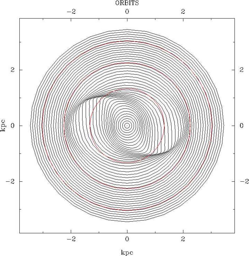
Figure 6: Orbits generated with Epic5. The red circles mark the oILR, corotation and OLR. The rotation is clockwise.

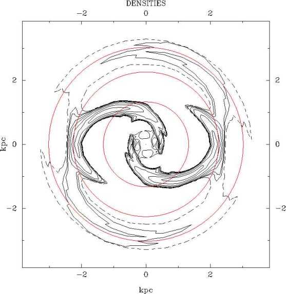
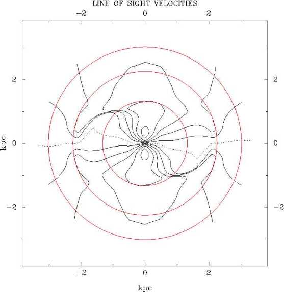
Figure 7: Left graph: Density contour $\rho/\rho_{1}$ in the plane of the galaxy. Contours at 0.99, 1.01, 1.02, 1.05, 1.1, 1.2, 1.4 and 1.7. Right graph: Velocity field in the plane of the galaxy with a position angle of 0^o and an increment of velocity between contours of 50 km s^-1. The direction of rotation is clockwise.

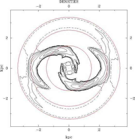
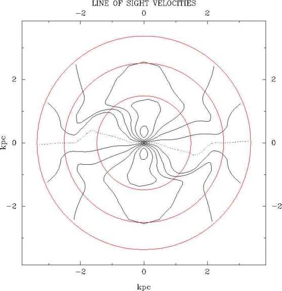
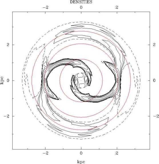
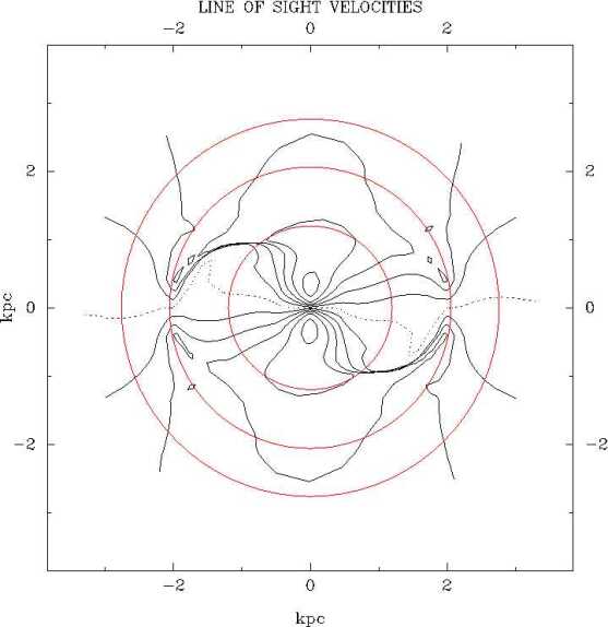
Figure 8: Upper and lower left graph: Density contour $\rho/\rho_{1}$ in the plane of the galaxy, for $\Omega_{p}$ equal to 60 km s^-1 kpc^-1and 80 km s^-1 kpc^-1, respectively. Contours at 0.99, 1.01, 1.02, 1.05, 1.1, 1.2, 1.4 and 1.7. Upper and lower right graph: Velocity field in the plane of the galaxy with a position angle of 0^o and an increment of velocity between contours of 50 km s^-1. Upper graph for a $\Omega_{p}$ equal to 60 km s^-1 kpc^-1 and lower for 80 km s^-1 kpc^-1. The direction of rotation is clockwise.

5 Epic5 applied to NGC 1365

To evaluate the limitations and abilities of Epic5 we want to compare it to hydrodynamic simulations of a nearby barred galaxy. For this, the strongly barred Seyfert galaxy NGC 1365 (Fig. 9) would be suitable. This galaxy has been extensively observed (see the review by P.O. Lindblad 1999) and a hydrodynamic simulation of the gas flow pattern was derived by LLA96. Also Zánmar Sánchez et al. (2008) observed and modeled the gas flow in the bar.

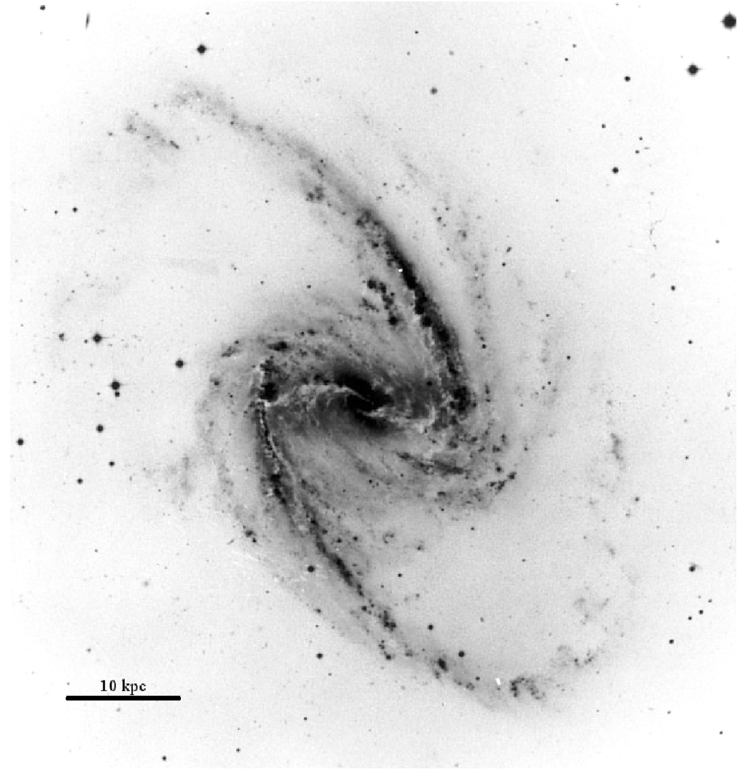
Figure 9: Optical image of NGC 1365 obtained at the prime focus of the ESO 3.6 m telescope.

A total hybrid velocity field has been derived by Lindblad et al. (1996) based on the HI velocity field of Jörsäter & van Moorsel (1995) and complemented with optical long slit spectra. We have here accepted the rotation curve based on this as derived by LLA96 (Fig. 10). It agrees closely with the rotation curve given by Zánmar Sánchez et al. (2008). We have derived the perturbed potential from the total surface density following the analysis using Bessel functions described in Binney & Tremaine (2008, Ch. 2.6.2) and LLA96 (their Appendix A). For this analysis, we used the Fourier series decomposition of the total surface density, obtained by LLA96 from a J-band image as given in their Figs. 7 and 9, and a normalized triangle density distribution along the vertical direction, with a $z_{0}$ scale parameter equal to 1 kpc. We smoothed the rotational velocity curve and the Fourier components along the radius and interpolated the curves in order to achieve enough resolution for the $\lambda_{2}$ criterion of the spiral potential (eq. 14). We use a clock-wise rotation in order to reproduce the observed galaxy.

When comparing with observations, we have taken the results given by Epic5, located in the galactic plane, and transformed them into the sky plane. For this purpose, we have used a position angle, PA, equal to 40^o and an inclination angle, $i$, of 42^o  (Jörsäter & van Moorsel 1995, also used in LLA96). In addition, we have assumed the systemic velocity to be 1632 km s^-1 and a scale of 0.1 kpc/arcsec.

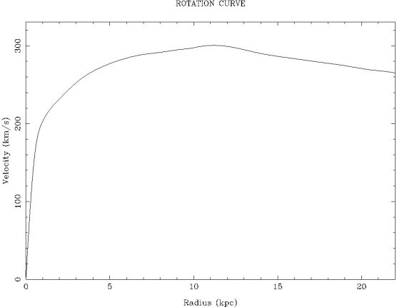
Figure 10: Rotational velocity curve of NGC 1365 (from LLA96).

5.1 Comparing with observations and simulations

The hydrodynamic simulations presented in LLA96 are performed using a flux-splitting 2nd-order code FS2, solving the flow of an ideal isothermal non-viscous gas (van Albada, 1985). LLA96 applies two different potentials derived from NGC 1365: bar only and bar + spiral. We have followed the same procedure in order to compare the results.

5.1.1 Bar potential

When deriving the bar only potential, only the cosine contributions to the Fourier series has been considered, and only up to a radius of around 100 arcsec, where the phase shift of the different modes start a steep increase (see Figs. 8, 9 and 11 in LLA96). The bar is positioned horizontally along the x-axis (Fig. 11, upper left).

As in LLA96, we have used a pattern speed of 20 km s^-1 kpc^-1. As illustrated in Fig. 11 (lower left), this pattern speed fixed the resonance radia to: the inner inner Lindblad resonance (iILR) at 0.4 kpc, the outer inner Lindblad resonance (oILR) at 2.7 kpc, the corotation radius (CR) at 14.4 kpc and the outer Lindblad resonance (OLR) at 21 kpc. We have used a constant friction coefficient $\lambda$ of 7 km s^-1 kpc^-1, and a corotation damping coefficient $\varepsilon$ of 5 km s^-1 kpc^-1. We are using an amplitude for the perturbing potential $\rm A_{\rm bar}=0.5$, half the amplitude used in LLA96. Thus, we have a potential with a bar strength, $|\Phi_{1}|_{\rm min}/|\Phi_{0}|_{\rm min}$, of 0.01. Increasing the bar amplitude, means that we have to increase the damping coefficients correspondingly to avoid self-crossing orbits, that are not realistic in a gaseous flow, and the results will be nearly the same. This may imply that the bar in NGC 1365 is actually too strong to be dealt with Epic5.

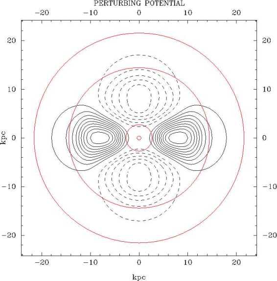
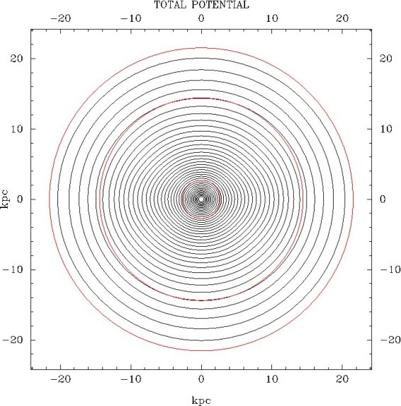
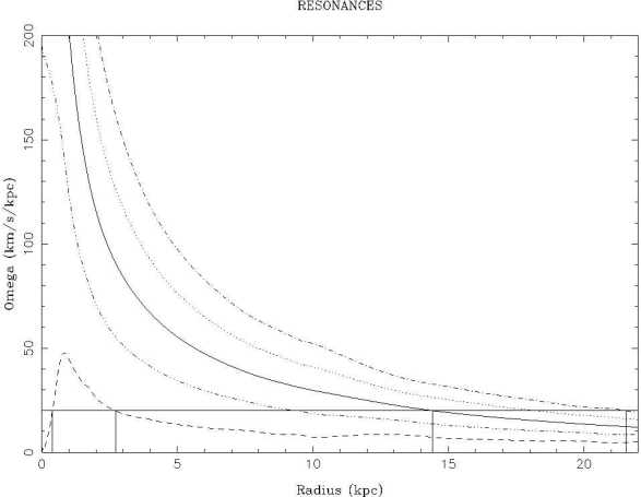
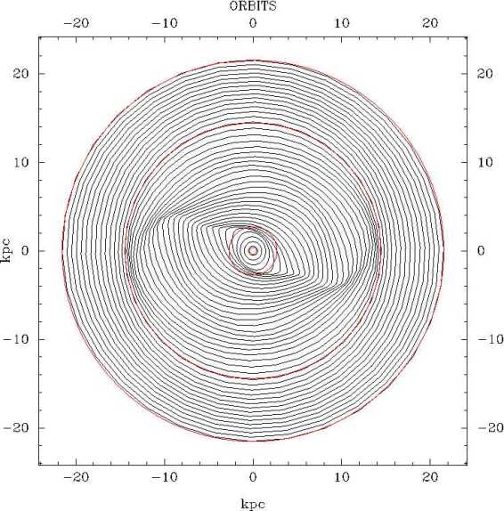
Figure 11: Upper left graph: Bar perturbing potential contours of NGC 1365, dashed lines correspond to positive contribution and solid lines to the negative contribution. Upper right graph: Total potential contours of NGC 1365 for a bar strength, $|\Phi_{1}|_{\rm min}/|\Phi_{0}|_{\rm min}$, of 0.01. Red curves: inner and outer Inner Lindblad Resonance (ILR), corotation and Outer Lindblad Resonance (OLR). Lower left graph: Angular velocities as in Fig. 5. The adopted pattern speed of 20 km s^-1 kpc^-1(horizontal solid line) is indicated as well as the positions of the resonances. Lower right graph: Orbits, seen as face-on, generated by Epic5 and the bar potential with a constant friction coefficient, $\lambda$, equal to 7 km s^-1 kpc^-1and a corotation damping coefficient, $\varepsilon$, of 5 km s^-1 kpc^-1.

Using these input parameters, we obtained with Epic5 the orbits, densities and velocity field shown in Fig. 11 and Fig. 12. The orbits are seen face-on. The density and velocity maps are projected on the sky plane, for comparison with the results of the simulations derived in LLA96 as well as with the observations.

We see from Fig. 11 (lower right) that the orbits in the region around oILR take elliptical shape, twisting in the counter rotation direction from being orientated at large angles to the bar, over 45 degrees at the oILR, to more elongated with the bar outside this resonance. Inside corotation matter circulates clockwise with respect to the bar, and the twisting and increasing deviation from elliptical shape gives rise to density increase forming a small trailing spiral across the oILR. This straightens out to a lane along the leading edge of the bar with sharp shock-like velocity jumps over the lane.

The influence of the inner 1:4 resonance, that occurs around R = 9 kpc, can also be seen in the orbits. Even the 1:6 resonance further out is discernible in the slight crowding of orbits. Strong crowding of orbits are seen at CR at the Lagrangian points L1 and L2 at the end of the bar and, with slightly spiral form, at the OLR in a direction perpendicular to the bar.

Compared to the orbits of the BM model of LLA96 (their Fig. 16), we see that between oILR and CR the BM orbits are more elongated and more orientated along the bar than ours. The 1:4 resonance is clearly seen also here. Around corotation the BM model displays the pendulum like motion referred to before and which is not reproduced by the linear approximation of Epic5.

The interstellar matter density map (Fig. 12 left graph), now projected on the sky plane, should be compared with the optical image of the galaxy (Fig. 9) and LLA96 (their Fig. 15). As expected from the orbits, the map shows a lane on the leading side of the bar that bends into spiral shape over the oILR. At the position of the 1:4 resonance a faint spur is seen, a strong arm appears at the end of the bar along the corotation radius, and a faint trailing arm extends out to the OLR. All these features have their correspondence in the BM density map of LLA96 (their Fig. 15). Fig. 12, right graph, shows the innermost region of the EPIC5 density map, where, as expected, a small nuclear leading spiral is seen across the iILR.

The velocity map, to be compared with LLA96 (their Fig. 20) is shown in Fig. 12 (middle graph). The map is projected on the sky plane with a line of nodes in PA 40^o and an inclination between the galaxy symmetry plane and the sky plane of $i$ = 42^o. The main difference, comparing the Epic5  result against the observations and simulations, is that the twisting of the zero velocity contour towards the bar is much weaker in the Epic5 case, which is connected with the different shapes of the orbits in the bar discussed above. This may partly be due to the difficulty of Epic5  to accept a very strong bar, as in NGC 1365, without getting crossing orbits. The behavior of the velocity contours inside the oILR are similar to that in LLA96, and the sharp velocity jumps, of the order of 100 km s^-1, in the lanes on the leading side of the bar are seen in all cases. The twisting of the contours along the spiral arms with velocity jumps on the inner side of the arms inside corotation are seen both in the simulations and in the Epic5 results.

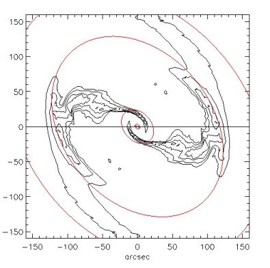
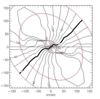
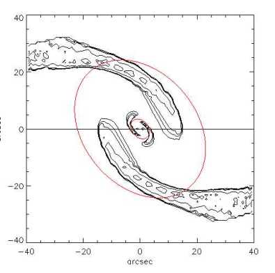
Figure 12: Left graph: Density ratio, $\rho/\rho_{0}$. Contours at 1.06, 1.2, 1.4 and 1.6. Middle graph: Line of sight velocity map derived by Epic5 using the position angle and the inclination of NGC 1365. Contours every 30 km s^-1, and thick solid line for the systematic velocity of the galaxy, 1632 km s^-1. Right graph: Density ratio, $\rho/\rho_{0}$, for the inner 4 kpc. Contours at 1.02, 1.04, 1.06, 1.2, 1.4 and 1.6. Maps seen projected on the sky plane.

5.1.2 Bar + Spiral potential

In the case of the bar + spiral potential we have taken the sine and cosine contribution of the Fourier series of the first three even modes until a radius of around 220 arcsec, just as described in LLA96. The resulting potential is seen in Fig. 13. We have used a pattern speed of 18 km s^-1 kpc^-1 (found for this potential by LLA96) and placed the bar horizontally along the x-axis. This pattern speed makes the resonance radia to be: the inner inner Lindblad resonance (iILR) at 0.38 kpc, the outer inner Lindblad resonance (oILR) at 3.1 kpc, the corotation radius (CR) at 15.8 kpc and the outer Lindblad resonance (OLR) at 23.5 kpc. We have chosen the coefficients $\lambda$ and $\varepsilon$ and parameter $A_{bar}$ the same as in the bar only case. The main difference between this case and the bar only case is that the spiral features are led much easier through corotation, which can be seen both in the orbits, Fig. 13 lower right graph, and the densities, Fig. 14 upper left graph. This was noticed also by LLA96.

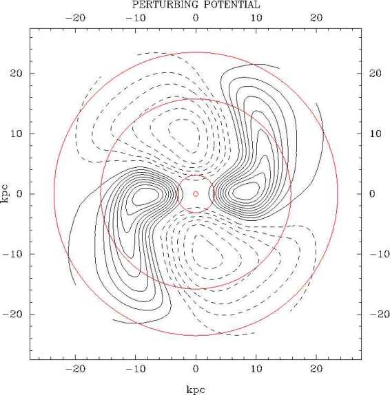
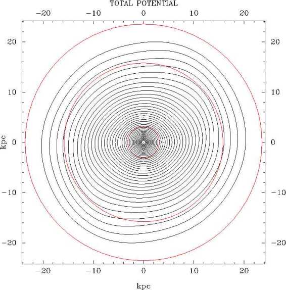
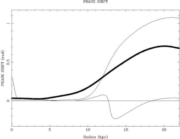
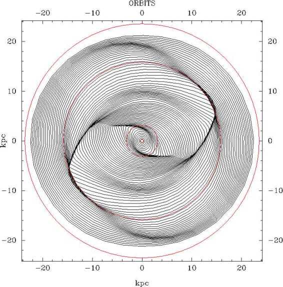
Figure 13: Upper left graph: Bar + spiral perturbing potential contours of NGC 1365. Upper rigth graph: Total potential contours of NGC 1365 corresponding to a perturbing strength of the potential, $|\Phi_{1}|_{\rm min}/|\Phi_{0}|_{\rm min}$, equal to 0.01. Red curves: inner and outer Inner Lindblad Resonance (ILR), corotation and Outer Lindblad Resonance (OLR). Lower left graph: Phase shift of the perturbed potential, $\vartheta_{m}(r)$, presented in the appendix A, for the three considered modes of its Fourier development. Thick solid line correspond to $m$ equal 2. Lower right graph: Orbits seen as face-on generated by Epic5 using the bar + spiral potential and a constant friction coefficient, $\lambda$, equal to 7 km s^-1 kpc^-1 and a corotation damping coefficient, $\varepsilon$, of 5 km s^-1 kpc^-1.

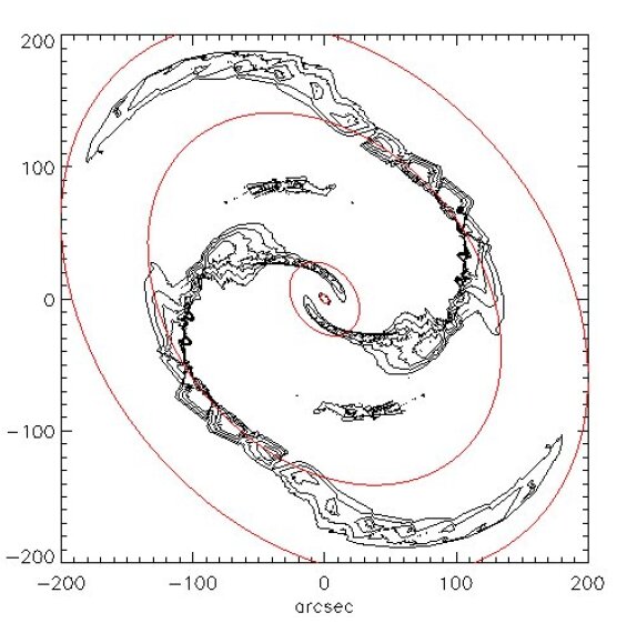
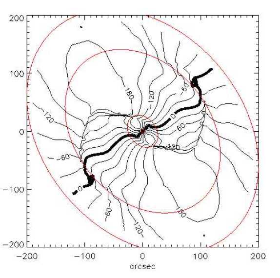
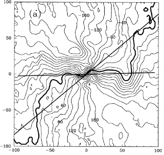
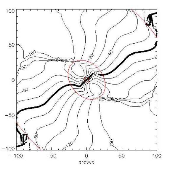
Figure 14: Upper left graph: Density ratio, $\rho/\rho_{0}$, for bar + spiral potential. Contours at 1.06, 1.2, 1.4 and 1.6. Upper right graph: Line of sight velocity map derived by Epic5  using the position angle and the inclination of NGC 1365. Contours every 30 km s^-1, and thick solid line for the systematic velocity of the galaxy, 1632 km s^-1. Lower left graph: Optical radial velocity field in the inner 100 arcsec of NGC 1365 taken from LLA96. Lower right graph: Line of sight velocity map derived by Epic5 for a bar + spiral potential in the inner 100 arcsec. Maps seen projected on the sky plane.

Fabry-Perot interferometry of NGC 1365, covering the H$\alpha$ regime has been obtained by Zánmar Sánchez et al. (2008). By kind permission we have got access to their total H$\alpha$ intensity data, which are reproduced in Fig. 15 (left map). In Fig. 15 (right map) we have for comparison color coded the Epic5  intensities from Fig. 14. Clearly the Epic5 model agrees well with the H$\alpha$ structure. The hot spots in the nuclear region and the active Seyfert nucleus is of course not reproduced by Epic5.

The velocity field obtained with Epic5 is shown in Fig. 14, together with the optical radial velocity field of NGC 1365 (inner 100 arcsec) taken from LLA96. In the innermost part, well inside the oILR, the contours indicate rapid rotation in nearly circular orbits. Between oILR and CR we again see how the isovelocity contours are concentrated to the leading edge of the bar. In the Epic5  case the contours are squeezed to a shock-like jump of about 100 km/s. The optical map cannot make such a sharp jump because it is smoothed due to the limited spatial resolution given by the limited set of long slits on which it is based. Over corotation we see similar shock behavior on the inner side of the spiral arms. The residual map obtained by subtracting the rotational velocity, Fig. 10, from the Epic5 model velocity field is presented in Fig. 16. In this Fig. 16 is also presented the residual velocities taken from Jörsäter & van Moorsel (1995). They subtracted from the observed HI velocity map, the rotational velocity derived from their observations considering a warp disc model after a radius of 250 arcsec. The general behavior is similar in the two cases with shocks along the bar and spiral arms. It is informative to compare the Epic5  map with the orbital map in Fig. 13 (lower right) to envision how the orbital circulation results in the observed line of sight velocity map.

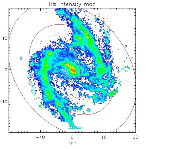
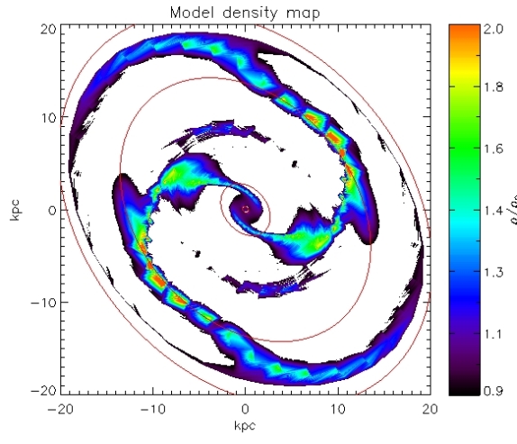
Figure 15: Upper left map: H$\alpha$ intensity map observed using a Fabry-Perot interferometer by Zánmar Sánchez et al. (2008). Shown in arbitrary units. Upper right map: Model density ratio $\rho/\rho_{0}$ obtained by Epic5 , eq. (12). Ratios lower than 0.9 are in white color.

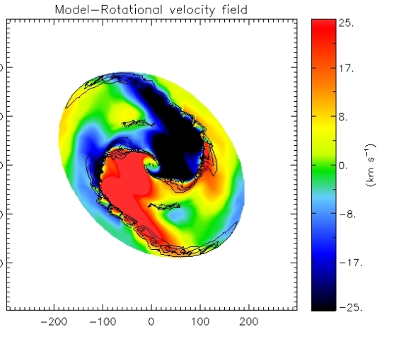
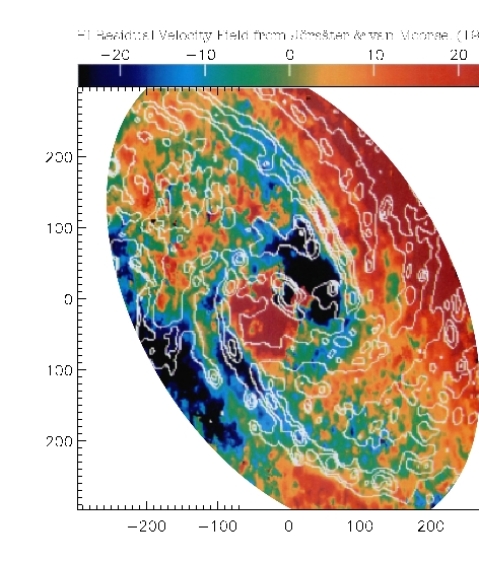
Figure 16: Left graph: Velocity model generated by Epic5 for a bar + spiral potential minus the rotational velocity from Fig. 10. Density contour over-plot in solid black lines. Right graph: HI velocity field observations minus rotational velocity model, figure from Jörsäter & van Moorsel (1995). The contours are from an optical image of NGC 1365. The NW side of the galaxy is the near one, and the rotation is clockwise. $x$-axis and $y$-axis in both graphs in arcsec.

6 Conclusions

Epic5 cannot fully replace elaborate hydrodynamical simulations. Epic5  solves the equations of motion in a solid body rotating, time independent galactic potential. This is done in the first order epicyclic approximation. Epic5  computes the deformation of the initially circular orbits of the guiding center, the velocity fields, and the structure created. Epic5  pictures a steady state created by a weak perturbing potential, it does not give the time evolution of galactic structure. Due to the degeneracy of the strength of the gravitational potential and damping coefficients, we can only derive relative values of the density.

Our comparison with a more elaborate simulation, as well as observations, show that it still can reproduce structural and dynamic properties. One of the advantages with Epic5, involving an analytic solution, is the speed by which it can survey the parameter space. Further, the possibilities, by varying parameters, to isolate artificially various agents important for forming structure of galaxies will be of importance for understanding the formation of galactic structure. Epic5 will be a useful complement to time consuming, elaborate simulations.

We would like to thank to J. A. Sellwood and R. Zánmar Sánchez for letting us use their H$\alpha$ data of NGC 1365. We also want to thank to the reviewer, Gene Byrd, for his useful comments. NP-F acknowledges financial support from NOTSA, and KF is supported by the Swedish Research Council (Vetenskapsrådet).

Appendix A Perturbations in the epicyclic approximation

We present in this paper a solution of the motion of a mass particle in an axisymmetric potential, $\Phi_{0}(r)$, with a weak non-axisymmetric perturbation, $\Phi_{1}(r,\theta)$. We assume that the potential is rotating with a pattern speed $\Omega_{\rm p}$, and we study the system in a corotating frame. We express the potential in polar coordinates:

$$\Phi(r,\theta)=\Phi_{0}(r)+\Phi_{1}(r,\theta)=\Phi_{0}(r)-\sum_{m=1}^{n}\Psi_{m}(r)\,\cos m(\theta-\vartheta_{m}(r))$$ (17)

where $\vartheta_{m}$ is the spiral phase. The rotation of the axisymmetric potential is about the center of gravity, which we have assumed to be at rest. Thus one has to be cautious in the presence of strong $m=1$ perturbation, when the center of mass could be significantly displaced.

In a corotating coordinate system we can write the equations of motions (see also Binney & Tremaine 2008, p.189):

$$\ddot{r}-r\dot{\theta}^{2} =-\frac{\partial\Phi}{\partial r}+2r\dot{\theta}\Omega_{p}+r\Omega_{p}^{2}$$ (18)

$$r\ddot{\theta}+2\dot{r}\dot{\theta} =-\frac{1}{r}\frac{\partial\Phi}{\partial\theta}-2\dot{r}\Omega_{p}$$ (19)

We introduce $\xi(t)$ and $\eta(t)$ as deviations from circular motion and write:

$$\centering r\@add@centering =r_{0}+\xi$$ (20)

$$\theta =\theta_{0}+(\Omega-\mbox{$\Omega_{\rm p}$})\,t+\frac{1}{r_{0}}\eta$$ (21)

where $\Omega$ is the circular angular velocity at a radius $r_{0}$. Assuming $\xi$ and $\eta$ to be small, and linearizing the equations of motion by neglecting higher order terms of $\xi$ and $\eta$, we get:

$$\centering\ddot{\xi}-2\Omega\dot{\eta}-4\Omega A\xi\@add@centering =-\frac{\partial\Phi_{1}}{\partial r}$$ (22)

$$\ddot{\eta}+2\Omega\dot{\xi} =-\frac{1}{r}\frac{\partial\Phi_{1}}{\partial\theta}$$ (23)

where $A$ is the Oort constant, $A=-r/2\,\,\,d\Omega/dr$.

To describe the motion of a gaseous medium, we introduce a frictional force proportional to the deviation from circular motion with a damping coefficient, $2\lambda$ (see Wada 1994, Lindblad & Lindblad 1994). With the introduction of this frictional force the equations of motion, eq. (22) and (23), are transformed into the equations (24).

$$\centering\ddot{\xi}+2\lambda\dot{\xi}-2\Omega\dot{\eta}-4\Omega A\xi\@add@centering =-\frac{\partial\Phi_{1}}{\partial r}=\sum_{m=1}^{n}\big{[}C_{m}\cos m(\theta-\vartheta_{m})+E_{m}\sin m(\theta-\vartheta_{m})\big{]}$$

$$\ddot{\eta}+2\Omega\dot{\xi}+2\lambda\dot{\eta}+4\lambda A\xi =-\frac{1}{r}\frac{\partial\Phi_{1}}{\partial\theta}=-\sum_{m=1}^{n}D_{m}\sin m(\theta-\vartheta_{m})$$ (24)

where

$$\centering C_{m}=\frac{d\Psi_{m}}{dr};\;\;\;\;\;\@add@centering D_{m}=m\frac{\Psi_{m}}{r};\;\;\;\;\;E_{m}=m\Psi_{m}\frac{d\vartheta_{m}}{dr}$$

Provided that we are not close to corotation, where $\Omega=\Omega_{p}$, we can assume that $\eta/r_{0}<<(\Omega-\Omega_{p})$, what makes

$$\theta\sim\theta_{0}+(\Omega-\mbox{$\Omega_{\rm p}$})\,t$$ (25)

with $\kappa^{2}=4\Omega^{2}-4\Omega A$, we can write the full solution of the now linearized eqs. (24) as:

$$\xi =ce^{-\alpha\lambda t}\cos\kappa(t-t_{0})+\sum_{m=1}^{n}\big{[}d_{m}\cos m(\theta-\vartheta_{m})+e_{m}\sin m(\theta-\vartheta_{m})\big{]}$$ (26)

$$\eta =-\frac{2\Omega}{\kappa}ce^{-\beta\lambda t}\sin\kappa(t-t_{0})+\sum_{m=1}^{n}\big{[}g_{m}\sin m(\theta-\vartheta_{m})+f_{m}\cos m(\theta-\vartheta_{m})\big{]}$$ (27)

$\alpha$ and $\beta$ are functions of $\Omega$ and $\kappa$, and $c$ is an arbitrary constant. The second terms on the left side of eqs. (26) and (27) give the forced oscillation due to the perturbing force. The first terms give the damped oscillation with the epicyclic frequency $\kappa$ around these guiding centra. We will leave out these latter terms in what follows and just consider the motions of the guiding center.

We introduce these eq. (26) and eq. (27) into (24), getting a system of equations with the 4$n$ unknown amplitudes, $d_{m}$, $e_{m}$, $g_{m}$ and $f_{m}$:

$$-(\omega_{m}^{2}+4\Omega A)d_{m}-2\omega_{m}\Omega g_{m} =C_{m}-2\lambda\omega_{m}e_{m}$$

$$-(\omega_{m}^{2}+4\Omega A)e_{m}+2\omega_{m}\Omega f_{m} =E_{m}+2\lambda\omega_{m}d_{m}$$

$$2\omega_{m}\Omega d_{m}+\omega_{m}^{2}g_{m} =D_{m}-2\lambda\omega_{m}f_{m}+4\lambda Ae_{m}$$

$$2\omega_{m}\Omega e_{m}-\omega_{m}^{2}f_{m} =-2\lambda\omega_{m}g_{m}-4\lambda Ad_{m}$$ (28)

where $\omega_{m}=m\,(\Omega-\mbox{$\Omega_{\rm p}$})$. The final solution is shown below.

$$d_{m} =\frac{(\kappa^{2}-\omega_{m}^{2})(\omega_{m}C_{m}+2\Omega D_{m})-2\lambda(\kappa^{2}+\omega_{m}^{2})E_{m}-4\lambda^{2}(\omega_{m}C_{m}-2\Omega D_{m})-8\lambda^{3}E_{m}}{\omega_{\varepsilon}\left[\left(\kappa^{2}-\omega_{m}^{2}\right)^{2}+8\lambda^{2}\left(\kappa^{2}+\omega_{m}^{2}\right)+16\lambda^{4}\right]}$$ (29)

$$g_{m} =\frac{-(\kappa^{2}-\omega_{m}^{2})\left[2\Omega\left(\omega_{m}C_{m}+2\Omega D_{m}\right)-\left(\kappa^{2}-\omega_{m}^{2}\right)D_{m}\right]+4\lambda\left[\left(\kappa^{2}-\omega_{m}^{2}\right)A+2\omega_{m}^{2}\Omega\right]E_{m}}{\omega_{\varepsilon}^{2}\left[\left(\kappa^{2}-\omega_{m}^{2}\right)^{2}+8\lambda^{2}\left(\kappa^{2}+\omega_{m}^{2}\right)+16\lambda^{4}\right]}$$

$$\;+\frac{-4\lambda^{2}\left[\left(\omega_{m}C_{m}+2\Omega D_{m}\right)\left(2\Omega-4A\right)-\left(\omega_{m}^{2}+3\kappa^{2}-8\Omega^{2}\right)D_{m}\right]+16\lambda^{3}AE_{m}}{\omega_{\varepsilon}^{2}\left[\left(\kappa^{2}-\omega_{m}^{2}\right)^{2}+8\lambda^{2}\left(\kappa^{2}+\omega_{m}^{2}\right)+16\lambda^{4}\right]}$$ (30)

$$e_{m} =\frac{\omega_{m}^{2}\left(\kappa^{2}-\omega_{m}^{2}\right)E_{m}+2\lambda\left[\left(\kappa^{2}+\omega_{m}^{2}\right)\left(\omega_{m}C_{m}+2\Omega D_{m}\right)-2\Omega\left(\kappa^{2}-\omega_{m}^{2}\right)D_{m}\right]-4\lambda^{2}\omega_{m}^{2}E_{m}+8\lambda^{3}\omega_{m}C_{m}}{\omega_{\varepsilon}^{2}\left[\left(\kappa^{2}-\omega_{m}^{2}\right)^{2}+8\lambda^{2}\left(\kappa^{2}+\omega_{m}^{2}\right)+16\lambda^{4}\right]}$$ (31)

$$f_{m} =\frac{2\omega_{m}\left(\kappa^{2}-\omega_{m}^{2}\right)\Omega E_{m}+2\lambda\left[4\omega_{m}\Omega\left(\omega_{m}C_{m}+2\Omega D_{m}\right)+\left(\kappa^{2}-\omega_{m}^{2}\right)\left(2AC_{m}-\omega_{m}D_{m}\right)\right]+8\lambda^{2}\omega_{m}E_{m}\left(\Omega-2A\right)+8\lambda^{3}\left(2AC_{m}+\omega_{m}D_{m}\right)}{\omega_{\varepsilon}^{2}\left[\left(\kappa^{2}-\omega_{m}^{2}\right)^{2}+8\lambda^{2}\left(\kappa^{2}+\omega_{m}^{2}\right)+16\lambda^{4}\right]}$$ (32)

At the Lindblad resonances $\kappa^{2}-\omega_{m}^{2}=0$, and we can see how the friction terms are damping the resonances when $\lambda\neq 0$. At corotation $\omega_{m}=0$. To damp this resonance, as explained in Section 2 in the paper, we have replaced $\omega_{m}$ in the denominator of eqs. (29) to (32) by $\omega_{\varepsilon}$, where

$$\frac{1}{\omega_{\varepsilon}}=\frac{\omega_{m}}{\omega_{m}^{2}+\varepsilon_{m}^{2}}$$ (33)

where $\varepsilon_{m}=m\varepsilon$ and $\varepsilon$ is an additional parameter.

References

- Adam et al. (1989) Adam G., Bacon R., Courtes G., Georgelin Y., Monnet G., Pecontal E., 1989, A&A, 208, L15
- Allington-Smith et al. (1997) Allington-Smith J. R., Content R., Haynes R., Lewis I. J., 1997, in A. L. Ardeberg ed., Society of Photo-Optical Instrumentation Engineers (SPIE) Conference Series Vol. 2871, Integral field spectroscopy with the Gemini Multiobject Spectrographs. pp 1284–1294
- Athanassoula (1992) Athanassoula E., 1992, MNRAS, 259, 345
- Bacon et al. (2001) Bacon R., Copin Y., Monnet G., Miller B. W., Allington-Smith J. R., Bureau M., Carollo C. M., Davies R. L., Emsellem E., Kuntschner H., Peletier R. F., Verolme E. K., de Zeeuw P. T., 2001, MNRAS, 326, 23
- Bacon et al. (1992) Bacon R., Emsellem E., Nieto J. L., Monnet G., 1992, Bulletin d’information du telescope Canada-France-Hawaii, 26, 11
- Binney & Tremaine (2008) Binney J., Tremaine S., 2008, Galactic Dynamics: Second Edition. Princeton University Press
- Boulesteix et al. (1987) Boulesteix J., Georgelin Y. P., Lecoarer E., Marcelin M., Monnet G., 1987, A&A, 178, 91
- Byrd et al. (2006) Byrd G. G., Freeman T., Buta R. J., 2006, A.J., 131, 1377
- Canzian (1993) Canzian B., 1993, Ap.J., 414, 487
- Fathi et al. (2005) Fathi K., van de Ven G., Peletier R. F., Emsellem E., Falcón-Barroso J., Cappellari M., de Zeeuw T., 2005, MNRAS, 364, 773
- Hernandez et al. (2003) Hernandez O., Gach J.-L., Carignan C., Boulesteix J., 2003, in M. Iye & A. F. M. Moorwood ed., Society of Photo-Optical Instrumentation Engineers (SPIE) Conference Series Vol. 4841, FaNTOmM: Fabry Perot of New Technology for the Observatoire du mont Megantic. pp 1472–1479
- Holmberg (1941) Holmberg E., 1941, Ap.J., 94, 385
- Jörsäter & van Moorsel (1995) Jörsäter S., van Moorsel G. A., 1995, A.J., 110, 2037
- Kormendy & Kennicutt (2004) Kormendy J., Kennicutt Jr. R. C., 2004, ARA&A, 42, 603
- Lin & Shu (1964) Lin C. C., Shu F. H., 1964, Ap.J., 140, 646
- Lindblad (1927) Lindblad B., 1927, Arkiv. matematik astronomi och fysik, Bd 20A, No. 17
- Lindblad (1958) Lindblad B., 1958, Stockholms Obs. Annaler, 20, No.6
- Lindblad (1963) Lindblad B., 1963, Stockholms Obs. Annaler, 22, No. 5
- Lindblad (1964) Lindblad B., 1964, Astrophys. Norvegica, IX, No. 12
- Lindblad et al. (1996) Lindblad P. A. B., Lindblad P. O., Athanassoula E., 1996, A&A, 313, 65 (LLA96)
- Lindblad (1960) Lindblad P. O., 1960, Stockholms Obs. Annaler, 21, No. 4
- Lindblad (1999) Lindblad P. O., 1999, A&ARv, 9, 221
- Lindblad et al. (2010) Lindblad P. O., Fathi K., Hjelm M., Nelson C. H., 2010, Ap.J., 723, 342
- Lindblad et al. (1996) Lindblad P. O., Hjelm M., Högbom J., Jörsaeter S., Lindblad P. A. B., Santos-Lleo M., 1996, A&A Suppl., 120, 403
- Lindblad & Lindblad (1994) Lindblad P. O., Lindblad P. A. B., 1994, in I. R. King ed., Physics of the Gaseous and Stellar Disks of the Galaxy, ASP Conference Series Vol. 66, . p. 29
- Loveday (1996) Loveday J., 1996, MNRAS, 278, 1025
- Roberts et al. (1979) Roberts Jr. W. W., Huntley J. M., van Albada G. D., 1979, Ap.J., 233, 67
- Sanders (1977) Sanders R. H., 1977, Ap.J., 217, 916
- Schoenmakers et al. (1997) Schoenmakers R. H. M., Franx M., de Zeeuw P. T., 1997, MNRAS, 292, 349
- Shlosman et al. (1989) Shlosman I., Frank J., Begelman M. C., 1989, Nature, 338, 45
- Shu et al. (1973) Shu F. H., Milione V., Roberts Jr. W. W., 1973, Ap.J., 183, 819
- van Albada (1985) van Albada G. D., 1985, A&A, 142, 491
- van de Ven & Fathi (2010) van de Ven G., Fathi K., 2010, Ap.J., 723, 767
- Wada (1994) Wada K., 1994, PASJ, 46, 165 (W94)
- Wong et al. (2004) Wong T., Blitz L., Bosma A., 2004, Ap.J., 605, 183
- Yih (1979) Yih C.-S., 1979, Fluid Mechanics: A Concise Introduction to Theory. West River Press, Ann Arbor
- Zánmar Sánchez et al. (2008) Zánmar Sánchez R., Sellwood J. A., Weiner B. J., Williams T. B., 2008, Ap.J., 674, 797