Strongly interacting one-dimensional bosons in optical lattices of arbitrary depth: From the Bose-Hubbard to the sine-Gordon regime and beyond

Abstract

We analyze interacting one-dimensional bosons in the continuum, subject to a periodic sinusoidal potential of arbitrary depth. Variation of the lattice depth tunes the system from the Bose-Hubbard limit for deep lattices, through the sine-Gordon regime of weak lattices, to the complete absence of a lattice. Using the Bose-Fermi mapping between strongly interacting bosons and weakly interacting fermions, we derive the phase diagram in the parameter space of lattice depth and chemical potential. This extends previous knowledge from tight-binding (Bose-Hubbard) studies in a new direction which is important because the lattice depth is a readily adjustable experimental parameter. Several other results (equations of state, energy gaps, profiles in harmonic trap) are presented as corollaries to the physics contained in this phase diagram. Generically, both incompressible (gapped) and compressible phases coexist in a trap; this has implications for experimental measurements.

Introduction — Ultracold atomic gases provide us with unprecedented experimental opportunities for creating interacting quantum many-particle systems bloch ; lewtool , both in lattice and in continuum situations. In response, theoretical lattice and continuum models have been widely analyzed in the past decade and half. However, it is experimentally straightforward to interpolate between the two cases, through periodic optical potentials whose amplitude can be made to vary from zero to a large value haller466pinning . The heating or cooling due to ramping up the strength of the periodic potential is well-studied heating_latticeloading . However, the potential well depth is generally not considered as a parameter tuning the phase diagram, except indirectly via effective Hubbard-model parameters which are strictly valid only in the deep-potential limit. The study of complex many-particle systems as a function of the periodic potential depth, interpolating between continuum and tight-binding limits, is a direction with many interesting effects whose exploration is just beginning. The measurements of Ref. haller466pinning are promising first steps in this direction. This experiment focuses on one-dimensional (1D) physics, where dimensional confinement enhances correlation and interaction effects.

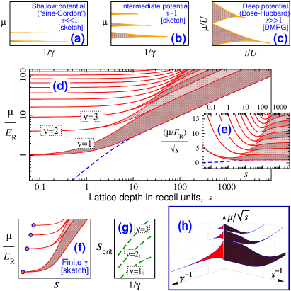
Figure 1: (a-c) Schematics of the $\mu$-$\gamma$ phase diagram for weak, intermediate and deep lattices. The Mott regions are shaded. The deepest lattice is taken to be described by a Bose-Hubbard model EjimaFehskeGebhard_EPL11 . (d,e) Calculated $\mu$-$s$ phase diagram for the strongly interacting ($\gamma^{-1}=0$) limit. Each Mott region corresponds to a different integer filling $\nu$. The dashed blue line is the energy of a single particle placed in an empty system, i.e., the chemical potential for $\nu=0$. (f,g) Inferred schematics for finite $\gamma^{-1}$: phase diagram and critical depths. (h) Structure of the 3D phase diagram (in $\mu$-$\gamma$-$s$ space) showing the ‘Bose-Hubbard’ region (previously studied) and the large-$\gamma$ plane (determined in this work).

In this work, we address the system implemented in the experiment of Ref. haller466pinning , namely, one-dimensional strongly interacting bosons in the presence of a variable-strength optical potential. We provide the most fundamental information needed for understanding the physics in this system, namely, the phase diagram.

Like many other systems, 1D bosons have been widely studied in the tight-binding and continuum limits Cazalilla::2011 , but not much for intermediate depths. The deep-well limit is described by the Bose-Hubbard model, which is a tight-binding model in the sense of each well being described by a single mode. The 1D Bose-Hubbard phase diagram is well-studied theoretically Cazalilla::2011 ; batrouni1996world ; freericks1994phase ; EjimaFehskeGebhard_EPL11 , and the model has been realized often experimentally bloch ; lewtool ; Cazalilla::2011 . In the other limit, i.e., without a periodic potential, the system is the continuum Lieb-Liniger gas LiebLiniger_1960 , described by the Hamiltonian $H=\sum_{j}\partial^{2}/\partial{x_{j}}^{2}+g\sum_{i<j}\delta(x_{i}-x_{j})$. The dimensionless interaction parameter is $\gamma=gm/(\hbar^{2}n)$, with $m$ the mass of bosons and $n$ the one-dimensional density. We are interested in large $\gamma$, in or near the so-called Tonks-Girardeau (TG) regime. The TG gas has been intensively studied theoretically Sen_pseudopotential ; brand2005dynamic ; Brand:PhysRevA72:2004 ; kolomeisky ; buljanlinear ; cazalilla2004differences ; Cazalilla::2011 ; Cazalilla:PhysicalReviewA:2003 ; Dunjko:2001p10842 ; Gangardt:NewJournalOfPhysics5:2003 ; Girardeau:1960p10745 ; paraan ; girardeauwright ; Papenbrock_PRA03 ; MinguzziGangardt_PRL05 . Some calculations exist in the weak lattice limit, via mapping to a sine-Gordon field theory kehrein_PRL99 ; lazarides2011 ; Buchler:2003p10714 . The TG gas has also been experimentally realized in a lattice version with low filling expt_TG_lattice . Ref. haller466pinning studies strongly interacting 1D bosons in the continuum, with the addition of a periodic potential of variable strength. Motivated by this, as well as by the dearth of theoretical studies of the effect of the potential depth, we analyze a Tonks-Girardeau gas in a periodic potential of variable depth. The periodic potential is $V(x)=sE_{R}\sin^{2}(qx)$, with lattice period $\pi/q$. The parameter $s$ gives the potential depth in units of the recoil energy, $E_{R}=\frac{\hbar^{2}q^{2}}{2m}$.

We use the Bose-Fermi transformation Girardeau:1960p10745 to map strongly interacting 1D bosons ($\gamma\rightarrow\infty$) to free fermions. The problem with a periodic potential then turns into a band-structure problem, which we address using the Bloch theorem. This rather simple setup allows us to extract a remarkable amount of information. The most prominent result is the phase diagram in the chemical potential ($\mu$) versus well depth ($s$) plane, i.e., we map out parameter regions which are Mott phases and those which are superfluid phases [Fig. 1(d,e)]. This phase diagram, whose structure to the best of our knowledge was not previously known, is exact and detailed in the $\gamma\rightarrow\infty$ limit, and also provides a significant amount of information about the phase diagram for finite but large $\gamma$.

We also present excitation gaps in the different Mott phases. Defining a “filling” variable $\nu$ as the average density in a well, we present equations of state, i.e, $\mu(\nu)$ curves, for various well depths. In addition, we calculate the effect of an arbitrary-strength periodic potential in the presence of an overall harmonic trap. This is important because, like Ref. haller466pinning , foreseeable experiments are likely to be performed in harmonic confinement. Going beyond the infinitely interacting case, we also provide results for large but finite interactions.

The phase diagram — Fig. 1(a-c) illustrate the phase diagram in the plane of chemical potential $\mu$ and (inverse) interaction strength, for weak, intermediate and strong lattice strength $s$. The deep-potential limit has been represented as the well-studied Bose-Hubbard model (top right). Away from this limit, the phase diagrams are expected to be of the forms sketched, but are not presently known in detail. It should be possible to determine parts of the small-$s$ phase diagrams using the sine-Gordon model, but full results do not yet exist in the literature.

Our calculation determines the small $\gamma^{-1}$ limit, i.e., the region touching the vertical axes in each of the top-panel schematics, for all values of the lattice depth $s$. This can be put into context in terms ofthe 3D phase diagram of Fig. 1(h): our calculation maps out a new plane in $\mu$-$\gamma$-$s$ space.

For $\gamma^{-1}=0$, the bosonic phase diagram is obtained from the free-fermion band structure. A filled fermionic band corresponds to integer filling in the bosonic system. Thus, the fermionic band-gap regions correspond to Mott phase regions in our system. The resulting exact phase diagram is shown in Fig. 1(d,e). This phase diagram is our main result.

The $s\rightarrow\infty$ region satisfactorily reproduces known features of the Bose-Hubbard limit — the Mott regions touch, killing superfluid regions, and each occupies an equal range of $\mu$. In the shallow “sine-Gordon” limit ($s\rightarrow{0}$), the Mott regions shrink to tiny slivers. For $\gamma^{-1}=0$ these Mott slivers continue down to $s=0$, so that an infinitesimal periodic potential can pin a gas if the filling allows commensurate pinning. In the $s=0$ limit, the successive Mott slivers appear at linearly increasing gaps of $\mu$ from each other.

In Fig. 1(f) we sketch the expected phase diagram for large but finite $\gamma$. The Mott regions now start at some finite critical lattice depth $s_{\rm crit}$. The Mott regions are expected to be less robust for larger fillings because of the smaller gaps and stronger perturbative corrections at larger $\nu$ (see below). It remains an open problem to determine the $s_{\rm crit}(\gamma)$ curves for $\nu>1$, sketched in 1(g). The $\nu=1$ curve can be obtained from a sine-Gordon description haller466pinning . The other curves should be be progressively higher [Fig.  1(g)] but are otherwise unknown.

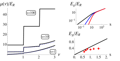
Figure 2: Left: Equation of state for various optical lattice depths. Solid curves correspond to $\gamma\rightarrow\infty$, dashed curves to $\gamma=11$. Right top: energy gaps $E_{g}$ in $\nu=1$, $\nu=2$ and $\nu=3$ Mott phases (top black, middle blue and bottom red) as a function of lattice depth. The gaps scale as $s^{\nu}$ at small $s$ and as $s^{1/2}$ at large $s$. Right bottom: calculated $\nu=1$ energy gap (line) shown with experimental values from trapped-system measurements haller466pinning .

Bose-Fermi mapping — To obtain the wavefunction of either $N$ hardcore bosons or $N$ noninteracting fermions in an arbitrary single-particle 1D potential, we take the first $N$ single-particle eigenfunctions $u_{i}(x)$. The many-body wavefunction is then $\psi_{f}(x_{1},x_{2},...,x_{N})=\sum_{P}\left(-1\right)^{P}\sum_{i}u_{i}(Px_{i})$ (where $P$ denotes a permutation) for fermions and $\psi_{b}(x_{1},x_{2},...,x_{N})=\sum_{P}\sum_{i}u_{i}(Px_{i})$ for bosons Girardeau:1960p10745 . Thus, we need to solve the single-particle Schrödinger equation with potential $V(x)=(x^{2}/2\ell_{\mathrm{tr}}^{2})+sE_{R}\sin^{2}(qx)$, where $\ell_{\mathrm{tr}}$ is the trap length for the harmonic trapping potential. For a uniform (non-trapped) system, the solution is known to be expressible in in terms of Mathieu functions Slater_PRB1952 ; Abramowitz .

Once the lowest $N$ single-particle orbitals $u_{i}(x)$ have been calculated, the one-dimensional density can be shown to be

$$n(y)=\int dx_{2}...dx_{N}\left|\psi(y,x_{2},...,x_{N})\right|^{2}=\sum_{i}u_{i}^{2}(y)\ .$$ (1)

The “filling factor”, the number of particles divided by the number of wells, is (for uniform systems) the integrated $n(x)$ over one period: $\nu=\int_{y}^{y+\pi/q}{dx}n(x)$. For non-uniform systems we assign to each well $j$ the filling $\nu(j)$, defined as the integral of $n(x)$ within that well.

Energy scales — For deep wells (large $s$), expanding $s\sin^{2}(qx)\approx sq^{2}x^{2}$ shows that the lower energy levels have equal spacing $\propto\sqrt{s}$. This implies equispaced bands, which explains the equal widths ($\propto\sqrt{s}$) of the Mott regions. On the other hand, for $s\rightarrow 0$, zero-point energy arises due to confinement by the neighboring particles. At filling $\nu$ this distance is $\pi/\nu{q}$ and therefore the relevant energy is $\nu^{2}E_{R}$. This explains the positions of the Mott slivers for $s\rightarrow 0$ and the linearly increasing distance between successive Mott regions [Fig. 1(d,e)].

Perturbation theory away from the Tonks-Girardeau point — Near the TG limit, i.e., for finite but large interactions, the 1D Lieb-Liniger gas can still be mapped onto a 1D weakly interacting fermionic problem. The fermionic interaction is unfortunately not simple. We use the form Sen_pseudopotential ; Brand:PhysRevA72:2004 ; brand2005dynamic ; paraan ; buljanlinear

$$\tilde{V}(x)=-\frac{2\hbar^{4}}{m^{2}g}\delta^{\prime\prime}(x)=-g_{f}\delta^{\prime\prime}(x).$$ (2)

This is to be interpreted as a perturbation to the fermionic state. Thus the energy shift for the bosonic ground state is $\delta E=\left<\psi_{f}\right|\tilde{V}\left|\psi_{f}\right>$. After some manipulation we obtain

$$\delta E=-\frac{g_{f}}{4}\int dR\,\left[g_{2}^{(2,0)}\left(R,R\right)-g_{2}^{(1,1)}\left(R,R\right)\right],$$ (3)

with $g_{2}^{(m,n)}$ denoting the $m$-th ($n$-th) derivatives with respect to the first (second) argument of the pair correlation function $g_{2}(x,y)$. For the TG gas, $g_{2}(x,y)=n(x)n(y)-\left|\Delta(x,y)\right|^{2}$ where $\Delta(x,y)=\sum_{i}u_{i}^{*}(x)u_{i}(y)$, the sum running over the first $N$ eigenstates girardeauwright .

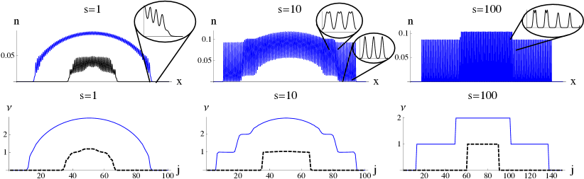
Figure 3: (Color online.) A harmonic trap in addition to the modulated potential. Top panels: densities $n(x)$, as a function of continuous position $x$. Bottom panels: fillings $\nu(j)$, as a function of discrete lattice index $j$. Blue curves are for 181 bosons. Lower black curves, where present, correspond to 31 bosons. The trap length is $30/\pi$ times the modulation period. Insets highlight features discussed in the text.

Equation of state — Fig. 2 (left) shows the chemical potential versus filling, for several different depths. We call these $\mu$ versus $\nu$ curves the “equations of state”. As the ground state is constructed by successively occupying single-particle states, the $\mu(\nu)$ curves are given by the single-particle energy dispersion curves (energy $\epsilon$ versus momentum $k$), with the interpretation $\nu=k/q$. The Mott regions are incompressible in the sense that the filling does not change with chemical potential, hence there are segments of these curves which are vertical jumps at integer values of $\nu$. The topography of the phase diagram — thin Mott regions for small $s$, thick Mott regions for large $s$ — is visible in the structure of these $\mu(\nu)$ curves.

We also show the perturbative correction to the equation of state curves for $\gamma$ large but finite. Specifically, we display $\gamma=11$, corresponding to some of the experimental data in Ref. haller466pinning . For small and moderate lattice strengths ($s\lesssim 10$), the corrections are minute. For $s\gg 10$, perturbative results are difficult to interpret and thus not displayed.

Excitation gap in Mott phase — Fig. 2 (right top) shows the first few energy gaps as a function of the trap depth when the system is in the Mott phase. The gaps correspond to the vertical jumps in the $\mu(\nu)$ curves (Fig. 2 left) or, equivalently, to the width of the Mott regions in Fig. 1. We find $E_{g}/E_{R}=\left|b_{\nu}(-\frac{s}{4})-a_{\nu}(-\frac{s}{4})\right|$, with $a_{\nu}$ and $b_{\nu}$ the characteristic values of Mathieu functions Abramowitz . For small $s$, the $\nu$-th gap grows as $s^{\nu}$, e.g., as ${s/2}$ and as $s^{2}/32$. For $\nu=1$ this is in agreement with sine-Gordon results haller466pinning ; kehrein_PRL99 ; Buchler:2003p10714 . For $s\gg{1}$, all gaps cross over to $\sim{s}^{1/2}$, in agreement with the energy-scale arguments given previously and consistently with Fig. 1(e).

The $\nu=1$ gap has been experimentally measured in haller466pinning through modulation spectroscopy. In Fig. 2 (right,bottom) we show the experimental data values (for $\gamma=11$) together with our exact calculation for $\gamma=\infty$. The perturbative result for $\gamma=11$ is indistinguishable from the TG line. Our results for trapped systems, below, show that a uniform-system gap cannot be expected to coincide with measurements on a trapped system with significant inhomogeneity.

An overall harmonic trap — In Fig. 3 we show the exact density profiles of a harmonically trapped Tonks-Girardeau gas in an optical lattice, for various lattice depths. We show both the densities $n(x)$ as a function of space and the fillings $\nu(j)$ as a function of well index. The fillings $\nu$ are obtained by averaging $n(x)$ over each well.

The fillings (bottom row) show a wedding-cake structure familiar from the literature on Bose-Hubbard physics in traps. It is noteworthy that we have obtained this from averaging densities in a continuum model, and not from a tight-binding model like the Bose-Hubbard. The $\nu(j)$ curves can be understood from “local density approximation” arguments based on the phase diagram presented in Fig. 1. Going from deeper to shallower modulations, the Mott regions grow thinner [Fig. 1(d,e)], and correspondingly there are smaller plateau regions in the density profiles. This resembles the effect of going from stronger to weaker interactions in the Bose-Hubbard model.

The continuum density profiles, $n(x)$, are less familiar from other contexts. The density oscillates at the lengthscale of the well size, so we have highlighted some features in insets. For ‘fillings’ larger than one, $n(x)$ within each well typically has multiple peaks. The height of the peaks in the $\nu=2$ plateau region is larger than, but not twice, that in the $\nu=1$ region. Only the filling $\nu(j)$, i.e., the integrated density, has integer values at the plateaus. Another feature is that the densities do not completely vanish between the wells, especially at small $s$, in neither superfluid nor Mott region.

In Fig. 4, we show profiles tailored to the experimental situation of Ref. haller466pinning , where the central tubes are reported to have about 60 bosons with maximal filling around $\nu\approx 1.2$. In a non-trapped (uniform) system at integer $\nu$, an arbitrarily weak modulation potential pins the whole system in a Mott state. Our results in Fig. 4 show that the situation is more complicated in a harmonic trap; $\nu$ is now strongly position-dependent. In particular, in the $s\lesssim 1$ regime, the part of the cloud which is ‘pinned’ at $\nu=1$ is a small fraction of the total. Therefore, identification of modulation spectroscopy measurements haller466pinning in this regime with a “Mott gap” is nontrivial. Further investigation incorporating inhomogeneity considerations is therefore called for. While Fig. 4 shows $\gamma=\infty$ results, the perturbative calculations in Fig. 2 indicate that corrections to the profiles will be tiny for interactions as low as $\gamma\sim 10$.

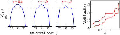
Figure 4: Left: Density profiles in a trap, with parameters corresponding to the central tube of the experiment of Ref. haller466pinning . Right: Mott fraction, defined as the number of sites with $|\nu-1|<\epsilon$ divided by the total number of bosons, with $\epsilon=0.02(0.05)$ for the lower (upper) curve.

Discussion; Open questions — We have studied strongly interacting bosons at and near the hardcore limit for periodic potentials of arbitrary depth. We have presented the phase diagram of the system in the $\mu$-$s$ plane, and quantitatively characterized various related aspects. By providing an exact and detailed map of one plane of the $\mu$-$\gamma$-$s$ space [Fig. 1(h)], we give a good first idea of the topography of this 3D phase diagram, and pave the way for future explorations of the complete 3D phase space.

Not surprisingly, the Mott regions are less dominant for weaker lattice strengths. This has clear consequences for trapped systems — the fraction of the system locked at integer values is small at small $s$. This may explain why the experimentally measured values for the $\nu=1$ gap fall below the theory for the uniform system. Heuristically, a significant part of the system is compressible (gapless), which may be expected to reduce the measured gap. Since the modulation spectroscopy employed in Ref. haller466pinning involves complicated temporal dynamics, this highlights the need for studies of time dependent properties of the non-uniform system with a weak lattice.

Other open questions raised by this work include the effects of non-infinite $\gamma$, beyond the perturbative calculations presented here. For $s\gg 10$, we find that the perturbative corrections at $\gamma\approx 10$ lead to the fermionic dispersion relation becoming non-monotonic, so that the Bose-Fermi mapping would involve careful (re-)interpretation. At small $s$, the perturbative calculation could in principle give estimates for the $s_{\rm crit}$ value where the Mott slivers end. (For $\gamma^{-1}=0$ the Mott slivers extend to $s=0$.) In practice, we have found that the perturbative corrections to the gap are so small that extensive high-precision computations would be required for such a calculation. A Monte Carlo or DMRG study, analogous to the 3D study of PilatiTroyer_arxiv1108 , would be useful in this regard.

Acknowledgments — We thank E. Haller and H.-C. Nägerl for providing us with experimental data.

References

- (1) I. Bloch, J. Dalibard, and W. Zwerger, Rev. Mod. Phys. 80, 885 (2008).
- (2) M. Lewenstein, A. Sanpera, V. Ahufinger, B. Damski, A. Sen, and U. Sen, Adv. Phys. 56, 243 (2007).
- (3) E. Haller, R. Hart, M. J. Mark, J. G. Danzl, L. Reichsöllner, M. Gustavsson, M. Dalmonte, G. Pupillo, and H.-C. Nägerl, Nature 466, 597 (2010).
- (4) M. Cramer, S. Ospelkaus, C. Ospelkaus, K. Bongs, K. Sengstock, and J. Eisert, Phys. Rev. Lett. 100, 140409 (2008); P. B. Blakie and A. Bezett, Phys. Rev. A 71, 033616 (2005).
- (5) M. A. Cazalilla, R. Citro, T. Giamarchi, E. Orignac, and M. Rigol, Rev. Mod. Phys. 83, 1405 (2011).
- (6) G. G. Batrouni and R. T. Scalettar, Computer Phys. Comm. 97, 63, (1996).
- (7) S. Ejima, H. Fehske, and F. Gebhard, Eur. Phys. Lett. 93, 30002 (2011).
- (8) J. K. Freericks and H. Monien, Europhys. Lett. 26, 545 (1994).
- (9) E. Lieb and W. Liniger, Phys. Rev. 130, 1605 (1963); E. Lieb, Phys. Rev. 130, 1616 (1963).
- (10) M. Girardeau, J. Math. Phys. 1, 516 (1960).
- (11) E. B. Kolomeisky, T. J. Newman, J. P. Straley, and X. Qi, Phys. Rev. Lett. 85, 1146 (2000).
- (12) D. Sen, Int. J. Mod. Phys. B 14, 1789 (1999); J. Phys. A 36, 7517 (2003).
- (13) J. Brand and A. Y. Cherny, Phys. Rev. A 72, 033619 (2005).
- (14) A. Y. Cherny and J. Brand, J. Phys.: Conf. Ser. 129, 012051 (2009).
- (15) F. N. C. Paraan and V. E. Korepin, Phys. Rev. A 82, 065603 (2010).
- (16) D. Jukić, S. Galić, R. Pezer, and H. Buljan, Phys. Rev. A 82, 023606 (2010).
- (17) M. A. Cazalilla, Phys. Rev. A 72, 033619 (2005).
- (18) M. A. Cazalilla, Phys. Rev. A 67, 053606 (2003).
- (19) V. Dunjko, V. Lorent, and M. Olshanii, Phys. Rev. Lett. 86, 5413 (2001).
- (20) M. D. Girardeau, E. M. Wright, and J. M. Triscari, Phys. Rev. A 63, 033601 (2001).
- (21) T. Papenbrock, Phys. Rev. A 67, 041601(R) (2003).
- (22) D. M. Gangardt and G. V. Shlyapnikov, New J. Phys. 5, 79 (2003).
- (23) A. Minguzzi and D. M. Gangardt, Phys. Rev. Lett. 94, 240404 (2005).
- (24) H. P. Buchler, G. Blatter, and W. Zwerger. Phys. Rev. Lett., 90, 130401 (2003).
- (25) A. Lazarides, O. Tieleman, and C. Morais Smith, Phys. Rev. A 84, 023620 (2011).
- (26) S. Kehrein, Phys. Rev. Lett. 83, 4914 (1999).
- (27) T. Kinoshita, T. Wenger, and D. S. Weiss, Science 305, 1125 (2004); B. Paredes, A. Widera, V. Murg, O. Mandel, S. Fölling, I. Cirac, G. V. Shlyapnikov, T. W. Hänsch, and I. Bloch, Nature (London) 429, 277 (2004).
- (28) J. C. Slater, Phys. Rev. 87, 807 (1952).
- (29) M. Abramowitz and I. A. Stegun (Eds.). ”Mathieu Functions.” Ch. 20 in Handbook of Mathematical Functions with Formulas, Graphs, and Mathematical Tables, 9th printing. New York: Dover, pp. 721-746, 1972.
- (30) S. Pilati and M. Troyer, arxiv:1108.1408.