Retroreflector Approximation of a Generalized Eaton Lens

Abstract

We extended a previous study of the Eaton lens at specific refraction angles to the Eaton lens at any refraction angle. The refractive index of the Eaton lens is complicated and has not analytical form except at a few specific angles. We derived a more accessible form of the refractive index for any refraction angle with some accuracy by retroreflector approximation. The finding of this study will be useful for a rapid estimation of the refractive index, and the the design of various Eaton lenses.

I Introduction

Trajectories of light can be controlled by prisms or a combination of mirrors, as well as by controlling the refractive index(RI) of a lens, such as GRIN(Gradient Index) lenses like the Eaton lens, Luneburg lens, and Maxwell’s fish-eye lens, etc.smoly It was once thought that the control of light trajectories was unrealistic or very difficult to realize, but recent developments of transformation optics and high RI materials from metamaterial techniques have provided novel methods for controlling wave trajectories.

The Eaton lens is a typical GRIN lens in which the RI varies from one to infinity. It has a singularity in that the RI goes to infinity at the center of the lens and it originates from a peculiar dielectric. The speed of light is reduced to zero at this point, and the lens can therefore, change the wave trajectories any direction.

The Eaton lens was recently studied at three specific refraction angles: $90^{o}$(right-bender), $180^{o}$(retroreflector), and $360^{o}$(time-delayer).hannay ; tomas ; danner The RI of the Eaton lens is given as a function of the radius, but it is not analytic except for at a few specific angles. Generally, the RI and its trajectories can only be obtained by numerical calculations. A simple but good approximation of the general form will be helpful for the design and application of Eaton lenses.

The RI of the Eaton lens is extended to arbitrary refraction angles. By combining a few Eaton lenses, we can construct an optical triangle, square, hexagon, or any geometric shaped path without mirrors. An extremely simple form of the RI is suggested within a reliable error range for easy and practical use by utilizing a linear approximation of the retroreflector.

II Generalized Eaton Lens

Hendi et al.hendi performed studies of light trajectories at central potentials. Based on the fact that the trajectory of the Eaton lens is an analogue of Kepler’s scattering problem (“scattering tomography”), they derived the relation between the light trajectory and its RI at any impact parameter. For symmetric and spherical lenses, the RI at the three specific refraction angles described above are known asdanner

Figure 1: The trajectories of Eaton lenses at three specific angles from Ref. danner . (A)$90^{o}$, (B)$180^{o}$, (C)$360^{o}$. Reprinted with permission from OSA.

$$n^{2} = \frac{1}{nr}+\sqrt{\frac{1}{n^{2}r^{2}}-1}\hskip 10.0pt (\theta=90^{o}),$$ (1)

$$n = \sqrt{\frac{2}{r}-1}\hskip 50.0pt (\theta=180^{o}),$$ (2)

$$\sqrt{n} = \frac{1}{nr}+\sqrt{\frac{1}{n^{2}r^{2}}-1}\hskip 9.0pt (\theta=360^{o}).$$ (3)

$n=1$ for $r\geq 1$, where $n$ is the relative RI. The $r$ is the radial position between 0 and 1, and the actual radial position is given by $ar$, where $a$ is the radius of the lens.

The importance of the above three lenses has been discussed previously. The right-bender in Eq. (1) has been studied in bending surface plasmon polaritons.zent The retroreflector in Eq. (2) is a device that returns the incident wave back to its source.ma The time-delayer in Eq. (3) is a time-clocking device in which the incident wave exits in the direction of the incidence as if the lens were not present. The trajectories for the above three cases was plotted by Danner and Leonhardtdanner and is shown in Fig. 1.

Figure 2: The refractive indexes at $\theta=90^{o},180^{o},270^{o}$, and $360^{o}$ from left to right.

Figure 3: The refraction angles at various refractive index and radius.

The RI of arbitrary refraction angles was derived from optics-mechanics analogy. RI is identical to particle trajectories of equal total energy $E$ in a central potential $U(r)$. The potential of the Eaton lens corresponds to the gravitation-like $U\propto-1/r$.hannay On the other hand the potential of the Luneburg lens corresponds to the harmonic-like $U\propto r^{2}$.morgan From the conservation of mechanical energy inside and outside the lens, the kinetic energy of a particle in the medium of RI $n$ is written as $(1/2)mn^{2}v^{2}=E-U$, where $m$ is the mass and $v$ is the velocity of the particle inside the lens. Then, $\int nds$ or $\int\sqrt{E-U}ds$ should be stationary bases on Fermat’s principle.

Replacing $\chi+\pi=\theta_{final}-\theta_{initial}$ into $\theta$ of Hannay and Haeusser’s equationhannay (See reference for the detailed derivation), we obtain a generalized form of the RI of the Eaton lens for arbitrary refraction angles as

$$n^{\pi/\theta}=\frac{1}{nr}+\sqrt{\frac{1}{n^{2}r^{2}}-1},$$ (4)

where $\theta$ is any radian angle and $n=1$ for $r\geq 1$. The refraction angle can be generalized as $\theta=(2N+1/2)\pi$ for the right-bender, $\theta=(2N+1)\pi$ for the retroreflector, and $\theta=2N\pi$ for the time-delayer, where $N$ is an integer. Note that $\theta=\pm\pi$ produces the same result with Eq. (2). We calculated RI numerically and plotted it at four specific angles in Fig. 2

Using the logarithm provides a more convenient form of the relation between RI and the radius.

$$\frac{\theta(n,r)}{\pi}=\frac{\log n}{\log\left(\frac{1}{nr}+\sqrt{\frac{1}{n^{2}r^{2}}-1}\right)}.$$ (5)

These relations are plotted in Fig. 3. A large RI changes trajectories at a small radius. The relation between RI and the radius is relatively more convenient to find using Eq. (5) than Eq. (4), but is still not practical for making a rapid estimation.

III Retroreflector Approximation

Figure 4: $p(r)$ as a function of radius. $\theta=90^{o},180^{o},270^{o}$, and $360^{o}$ from top to bottom. $p(r)$ is linear for $\theta=180^{o}$.

Introducing a new radial function $p(r)$, the nonlinear Eqs. (4) and (5) are used as a more accessible form. From Eq. (4) we obtain $n(r)$ at two boundaries. As $r\sim 0$, then $n\sim(2/r)^{\theta/(\pi+\theta)}$. As $r\sim 1$, then $n\sim(1/r)^{\theta/(\pi+\theta)}$. Therefore, we can write $n(r)$ for the range of $0<r\leq 1$ in the following compact form

$$n(r)=\left\{\frac{p(r)}{r}\right\}^{\frac{\theta}{\pi+\theta}},$$ (6)

where $0<p(r)\leq 1$. The new variable $p(r)$ is plotted in Fig. 4.

The time-delayer with $\theta=2N\pi$ is an invisible sphere. The general form with an $N$ turn can be represented easily using $p(r)$ in Eq. (6). When it has an $N$ turn, the time delay $\triangle\tau$ is obtained as

$$\triangle\tau=\frac{2N\pi rn}{v_{o}}=\frac{2N\pi r}{v_{o}}\left\{\frac{ap(r)}{r}\right\}^{\frac{2N}{2N+1}},$$ (7)

where $v_{o}$ is the background velocity outside the lens and $a$ is the radius of the lens. If $N\gg 1$, then $2N\pi a/v_{o}\leq\triangle t\leq 4N\pi a/v_{o}$. Therefore, $a$ and $N$ are the two main factors that decide the time cloaking or delay properties.

As $p(r)$ is a function of the radius, we can introduce an approximation. From Eq. (6) $p(r)$ can be written as

$$p(r)=rn(r)^{\frac{\pi+\theta}{\theta}}.$$ (8)

It is a bounded and analytic function of the radius between 1 and 2. Every line is monotonically decreasing from $r=0$ to $r=1$ and nearly linear. Therefore, we can take the retroreflector approximation or a linear approximation as

$$p(r)\simeq 2-r.$$ (9)

Substituting Eq. (9) into Eq. (6), we obtain the simple form of the RI at any refraction angle as

$$n(r)\simeq\left(\frac{2}{r}-1\right)^{\frac{\theta}{\pi+\theta}}.$$ (10)

Figure 5: Comparison between the exact value obtained by numerical calculation and the retroreflector approximation for $\theta=90^{o},270^{o}$. The error is less than 4$\%$ at $\theta=90^{o}$, and less than 5 $\%$ at $\theta=270^{o}$. They match exactly at the both ends of $r\rightarrow 0,1$ at every angle.

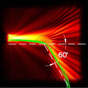
Figure 6: Optical path at $\theta=60^{o}$ by the retroreflector approximation in Eq. (10). The plot was generated using a COMSOL simulator.

The effectiveness of the approximation is examined by comparison with the exact values obtained from the numerical calculations in Fig. 5 and the optical path was plotted for $\theta=60^{o}$ in Fig. 6. The error of Eq. (10) is less than 4$\%$ at $\theta=90^{o}$, 5$\%$ at $\theta=270^{o}$, and 10$\%$ at $\theta=360^{o}$. The error accumulates for more than $360^{o}$ and less than $0^{o}$. Therefore, this calculation is useful at the conventional angle ranges of $0<\theta<2\pi$ within a 10$\%$ error.

IV Conclusions

The Eaton lens is a typical GRIN lens with a complicated RI. We extended previous studies of the Eaton lens at specific refraction angles to any refraction angle. The RI refractive index of the Eaton lens is complicated and not analytical except for a few specific angles. We derived a more accessible form of the RI for any refraction angles using the retroreflector approximation. This method is applicable at conventional angle ranges of $0<\theta<2\pi$ within a $10\%$ error. It is extremely simple but useful for a rapid estimation of optical properties obtained from the RI.

References

- (1) V. N. Smolyaninova, I. I. Smolyaninov, A. V. Kildishev, and V. M. Shalaev, Maxwell fish-eye and Eaton lenses emulated by microdroplets, Opt. Lett. 35 (2010) 3396.
- (2) J. H. Hannay and T. M. Haeusser, Retroreflection by refraction, J. Mod. Opt. 40 (1993) 1437.
- (3) T. Tyc and U. Leonhardt, Transmutation of singularities in optical instruments, N. J. Phys. 10 (2008) 115038.
- (4) A. J. Danner and U. Leonhardt, Lossless design of an Eaton lens and invisible sphere by transformation optics with no bandwidth limitation, 2009 Conference on Lasers and Electro-Optics(CLEO), Baltimore, MD, U. S. A. (2009).
- (5) A. Hendi, J. Henna, and U. Leonhardt, Ambiguities in the Scattering Tomography for Central Potentials, Phy. Rev. Lett. 97 (2006) 073902.
- (6) T. Zentgraf, Y. Liu, M. H. Mikkelson, J. Valentine, and X. Zhang, Plasmonic Luneburg and Eaton lenses, Nature, Nano, 6 (2011) 151.
- (7) Y. G. Ma, C. K. Ong, T. Tyc, and U. Leonhardt, An omnidirectional retroreflector based on the transmutation of dielectric singularities, Nature, Mat. 8 (2009) 639.
- (8) S. P. Morgan, General Solution of the Luneberg Lens Problem, J. Appl. Phys. 29 (1958) 1358.