Structure factors in granular experiments with homogeneous fluidization

Abstract

Velocity and density structure factors are measured over a hydrodynamic range of scales in a horizontal quasi-2d fluidized granular experiment, with packing fractions $\phi\in[10\%,40\%]$. The fluidization is realized by vertically vibrating a rough plate, on top of which particles perform a Brownian-like horizontal motion in addition to inelastic collisions. On one hand, the density structure factor is equal to that of elastic hard spheres, except in the limit of large length-scales, as it occurs in the presence of an effective interaction. On the other hand, the velocity field shows a more complex structure which is a genuine expression of a non-equilibrium steady state and which can be compared to a recent fluctuating hydrodynamic theory with non-equilibrium noise. The temporal decay of velocity modes autocorrelations is compatible with linear hydrodynamic equations with rates dictated by viscous momentum diffusion, corrected by a typical interaction time with the thermostat. Equal-time velocity structure factors display a peculiar shape with a plateau at large length-scales and another one at small scales, marking two different temperatures: the “bath” temperature $T_{b}$, depending on shaking parameters, and the “granular” temperature $T_{g}<T_{b}$, which is affected by collisions. The two ranges of scales are separated by a correlation length which grows with $\phi$, after proper rescaling with the mean free path.

I Introduction

Understanding granular systems is strategically relevant for the optimization of many industrial processes in pharmaceutical, food, cosmetic, chemical, petroleum, polymer and ceramic industries Duran (2000); Jaeger et al. (1996). It is also essential for modeling geophysical phenomena such as sediment fluidization in landslides Scholz (1998); Iverson (1997); Johnson and Jia (2005) and soil mechanics Khaldoun et al. (2005). Finally, it is a challenge in the field of statistical physics of out-of-equilibrium complex materials Kadanoff (1999); Kudrolli (2008); Nowak et al. (1997); Biroli (2007); Keys et al. (2007a); Candelier and Dauchot (2009). Experimental granular materials are usually limited to a few thousands particles, sometimes even less Goldhirsch (1999); Kadanoff (1999). Because of this inherently “small” system size, fluctuations in granular experimental systems are rarely negligible and should be considered in the analysis.

Usually there is no general theory available to describe fluctuations in non-equilibrium stationary systems (NESS) McLennan (1989); Zwangzig (2001); Bertini et al. (2002). A NESS is obtained in general by applying a steady driving force to a thermostatted system of interest: that results in a macroscopic breakdown of time-reversal accompanied by directed currents. The typical situation, within the realm of molecular fluids, is by steady shearing – giving place to a transverse momentum current – or by contact with two thermal reservoirs at different temperatures – leading to a steady current of heat Schmitz and Cohen (1985); de Zarate and Sengers (2006). Therefore, molecular fluids are characterized by non-equilibrium conditions associated in general to spatially non-homogeneous configurations, i.e. currents appear in physical space and break isotropy or other spatial symmetries.

An entirely different situation is present in so-called active matter, which includes driven granular materials, as well as “fluids” of pedestrians, flocks of animals (birds or fish), suspensions of bacteria or network of filaments (e.g. actin) in the cell, etc. Toner et al. (2005); Narayan et al. (2007); Jülicher et al. (2007); Cavagna et al. (2010) Common properties of those systems are the presence of non-conservative interactions, often mediated by a solvent, and of an external energy injection which can be – in principle – spatially homogeneous (for instance, animal or bacteria express their self-propulsion in the bulk of the system and not only at its boundaries). The situation with granular materials depends on the setup: experiments exist where most of the grains are in contact with the external energy source irrespectively of their position Olafsen and Urbach (1998); Prevost et al. (2002); Reis et al. (2007); Rivas et al. (2011), resulting in a spatially homogeneous NESS.

The present paper is devoted to investigate the structure of the velocity field in an experimental setup, which realizes an homogeneous driving mechanism, already discussed in Gradenigo et al. (2011a). In homogeneous molecular fluids, the velocity field is not expected to display any structure, as a consequence of the separation of the Hamiltonian into a kinetic and a potential part $\mathcal{H}=\mathcal{K}+\mathcal{U}$, the former being furtherly separated in single-particle additive contributions, $\mathcal{K}=\sum_{i}K_{i}$, that gives place to a factorized Maxwell-Boltzmann kinetic distribution $\sim\prod_{i}\exp(-\beta K_{i})$, with no inter-particle velocity correlations and temperature $1/\beta$. On the contrary, granular fluids are characterized by non-conservative interactions (kinetic energy is dissipated in collisions), often resulting in inter-particle velocity correlations, as well as velocity-position cross-correlations: such effects are best appreciated in not too dilute setups, where they give origin to visible non-equilibrium peculiarities, such as for instance the violation of the Einstein fluctuation dissipation theorem (FDT) Puglisi et al. (2007). Velocity correlations in a similar granular setup have been previously studied in Prevost et al. (2002), measuring them in direct space and – therefore – focusing on small spatial distances. In this paper we shall focus on the study of structure factors (in $k$-space), since it highlights large space-time scales and is therefore more suitable to compare the experimental results with theory. Nevertheless the results of Prevost et al. (2002) are compatible with those presented here (and in our previous publication Gradenigo et al. (2011a)), in the observation of exponentially space-dependent velocity correlations for the case of a rough vibrating plate.

Our experiments are also interesting to discriminate between two models of “granular thermostats” which differ for the presence/absence of a viscous drag force (per unit of mass) $-\gamma_{b}{\bf v}_{i}$ proportional to the velocity ${\bf v}_{i}$ of the $i$-th particle: the presence of such a term allows one to define a typical interaction time $1/\gamma_{b}$ with the thermostat and a finite “bath” temperature $T_{b}$ (see the discussion in Section IV.4). The experiment with a rough plate is well described by a model with $\gamma_{b}>0$, and an effective bath temperature can indeed be measured by looking at scales larger than a well-defined correlation length.

This paper has the following organization: in Section II the experimental setup and the protocols of measurements are explained. In Section III the probability distributions of velocities are presented. The measurements of density, transverse and longitudinal velocity structure factors are discussed in Section IV. From a comparison of those structure factors with a phenomenological fluctuating hydrodynamic theory, we get access to transport coefficients, bath temperature and some typical non-equilibrium correlation lengths. The dependence of those quantities with external parameters are investigated in Section V. Concluding remarks appear in Section VI.

II Experimental details

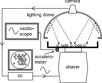
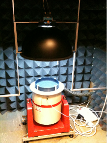
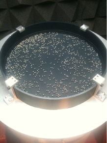
Figure 1: Left: a logical scheme of the experiment. Center and right: two pictures of the experimental setup.

In the left frame of Fig. 1 a rationale of the experiment is presented. The center and right frames reproduce real photographs of the setup. See video1 and video2 for movies representing the time-evolution of the system with different experimental parameters. The energy source is an electrodynamic shaker, model V450 by LDS Test & Measurement, placed on top of a support with tunable inclination by means of adjustable feet. An aluminum mounting plate is placed over the head of the shaker. The container of the granular media, which is fixed over the mounting plate, is a circular aluminum plate with diameter $D=$200\text{\,}\mathrm{mm}$$, with perpendicular borders (whose height, $20\text{\,}\mathrm{mm}$, is however irrelevant for the present setup). The final horizontal alignment is verified, directly on top of the plate carrying the granular sample, by means of a spirit level with a precision of $0.02\text{\,}\mathrm{mm}\text{\,}{\mathrm{m}}^{-1}$. The alignment check is repeated after every single run. The container has been produced to have a flat floor and then it has been submitted to sandblasting procedure with corundum mixture (aluminum oxide) whose nominal grain size is $1190\text{\,}\mathrm{\SIUnitSymbolMicro m}$, also called “gr16”: actually, such a sand is highly polydisperse (grains as small as $200\text{\,}\mathrm{\SIUnitSymbolMicro m}$ can be found in it), and the rough surface created in the sandblasting process presents holes with sizes in the range [$50\text{\,}\mathrm{\SIUnitSymbolMicro m}$, $500\text{\,}\mathrm{\SIUnitSymbolMicro m}$], as checked by means of an optical microscope. Finally, a black coating is applied by electrochemical burnishing in order to enhance contrast for particle visualization. The shaker is fed, through an amplifier PA1000 (LDS), with a sinusoidal signal at frequency $f$, which is converted in a sinusoidal force applied to the payload. This appears as a sinusoidal movement of the plate with amplitude $A$, i.e. $z(t)=A*\sin(2\pi ft)$, where $z(t)$ is the vertical coordinate of the plate at time $t$. Provided a linear response of the amplifier and of the shaker, a given maximum amplitude of the input signal together with a given mass of the payload determine a maximum acceleration $\ddot{z}_{max}=A(2\pi f)^{2}$. For instance, with all other parameters kept constant, a change of frequency results in a change of amplitude of oscillation $A\sim 1/f^{2}$. Our experiments are done at frequencies in the range $[150,250]\text{\,}\mathrm{Hz}$ and accelerations, in units of gravity acceleration $g$, in the range $[5,11]$. We have verified that, within those limits, the system remains in a quasi-2d regime, with a negligible number of particles flying at heights larger than their diameter. Peak to peak acceleration is measured during the course of each run (i.e. with full payload, including moving particles) by means of an accelerometer, placed on the mounting plate, connected to a digital averaging oscilloscope in order to remove the spikes due to particle-plate collisions.

The imaging apparatus consists of a fast camera, placed above the central point of the container, and a lighting dome: the former is an EoSens CL from Mikroron, the latter, placed at height much above the layer of particles (and therefore not interacting with them), is made of a led ring whose emitted light is reflected by a diffusing half-spherical surface, reaching the granular medium with a high degree of isotropy and uniformity. As seen in the right frame of Fig. 2, a very weak radial density gradient is present, so that particles in the central region are slightly less concentrated than those near the border. For the sake of verifying the importance of such a weak spatial inhomogeneity, we have performed measurements both in the whole container (e.g. right frame of Fig. 2) and in a restricted region focusing on a central rectangular “region of interest” (roi), of size $L_{x}\times L_{y}=$100\text{\,}\mathrm{mm}$\times$100\text{\,}\mathrm{mm}$$ (e.g. left frame of Fig. 2). Changing the optics and the distance of the camera, we manage to get, in both cases, a digital image with dimensions $840\times 840$ pixels. Results obtained with the two different “roi”, shown in the following sections, do not display qualitative differences but only weak quantitative discrepancies due to small non-homogeneities. Nevertheless, a larger “roi” allows one to probe modes with larger wavelengths, which is relevant in the comparison with theoretical predictions for structure factors at small wave-vectors. A very weak radial density gradient is visible in Fig. 2, due to the presence of hard boundaries where dissipation is stronger and density may be slightly enhanced.

Particles used in this experiment are restricted to a single material and a few sizes, varying packing fraction, i.e. varying their number $N$, and shaking parameters. Here, we use spheres with diameter $\sigma$ in the range $[1,4]$ mm made of “$316$-steel”, which is non-magnetic in order to avoid interference with the shaker electromagnet. Before each experimental run, particles and container are washed in a ultrasound machine to eliminate those impurities which spoil the reproducibility of the experiment: indeed, the effectiveness of energy transfer between vertical vibration and horizontal spheres motion is mediated by frictional properties of the sphere-surface contact, which could be changed by cleanness of the apparatus.

Steel reflectance properties are such that each particle appears as a bright and well defined spot, smaller than its diameter. A simple lookup table is sufficient to segment the image distinguishing the interesting white blobs (particles) from the black background. Particles appear as almost-circular blobs with an average diameter $d_{blob}$ – reported in Table 1 – ranging from $\sim 2$ to $\sim 8$ pixels. The frame-rate $f_{acq}$ used for image acquisition is in between $[60,250]$ frames per second. Reasons for the choice of space and time resolution are discussed below.

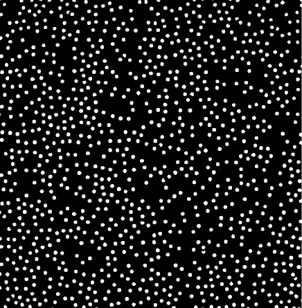
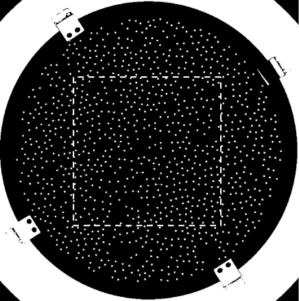
Figure 2: Two pictures from the acquisition camera (enhanced online). Left: zoom on the central region of interest. Right: whole system (refer also to Table 1). The dashed box marks the zoomed region.

As mentioned above, the system of interest, here, is a projection of the granular sample on the horizontal plane: only horizontal positions and velocities are measured. It is directly observed that particles never go on top of each other, allowing to consider this system as a quasi-$2$-dimensional fluid, also in the absence of a top lid.

The parameters used in the present paper are resumed in Table 1. To have an idea of the relevance of interactions, we also report the mean free path $\lambda=1/(2\sqrt{\pi}g_{2}n\sigma)$, where $n$ is number density on the plane and $g_{2}$ the value of the equilibrium pair correlation function at contact. A label is assigned to each experimental configuration in order to be easily referred to in the rest of the discussion. The rationale of the set of experiment is the following: experiments A-H are done with diameter $2\text{\,}\mathrm{mm}$, I-T are with diameter $1\text{\,}\mathrm{mm}$, U-X are with diameter $4\text{\,}\mathrm{mm}$; experiments A-H and I-P focus on a central region, while Q-X focus on the whole system; experiments A-D, I-L, Q-T and U-X are groups of four configurations where only the packing fraction is changed, from $10\%$ to $40\%$; experiments E-H and M-P are performed at constant packing fraction, but varying the shaking parameters (frequency or maximum acceleration).

Label	$N$	$\sigma$	$\phi$	$\lambda$	$f$	$z_{max}$	$\dot{z}_{max}$	$\frac{\ddot{z}_{max}}{g}$	$f_{acq}$	roi	$d_{blob}$	$\delta$	$\delta$
		(mm)		(mm)	(Hz)	(mm)	(mm/s)		(Hz)		(pixel)	(pixel)	(mm)
A	1000	2	10%	3.75	200	0.039	49.1	6.3	250	center	8.368	0.346	0.041
B	2000	2	20%	1.55	200	0.039	49.1	6.3	250	center	8.368	0.346	0.041
C	3000	2	30%	0.83	200	0.039	49.5	6.3	250	center	8.368	0.346	0.041
D	4000	2	40%	0.48	200	0.039	49.5	6.3	250	center	8.368	0.346	0.041
E	3000	2	30%	0.83	150	0.070	65.5	6.3	250	center	8.368	0.346	0.041
F	3000	2	30%	0.83	250	0.026	40.6	6.5	250	center	8.368	0.346	0.041
G	3000	2	30%	0.83	200	0.048	60.8	7.8	250	center	8.368	0.346	0.041
H	3000	2	30%	0.83	200	0.031	39.0	5.0	250	center	8.368	0.346	0.041
I	4000	1	10%	1.88	200	0.039	48.7	6.2	250	center	4.514	0.471	0.056
J	8000	1	20%	0.78	200	0.039	48.7	6.2	250	center	4.514	0.471	0.056
K	12000	1	30%	0.42	200	0.039	49.1	6.3	250	center	4.514	0.471	0.056
L	16000	1	40%	0.24	200	0.039	49.5	6.3	250	center	4.514	0.471	0.056
M	12000	1	30%	0.42	150	0.068	64.5	6.2	250	center	4.514	0.471	0.056
N	12000	1	30%	0.42	250	0.026	40.6	6.5	250	center	4.514	0.471	0.056
O	12000	1	30%	0.42	200	0.048	60.8	7.8	250	center	4.514	0.471	0.056
P	12000	1	30%	0.42	200	0.031	39.4	5.0	250	center	4.514	0.471	0.056
Q	4000	1	10%	1.88	200	0.039	48.7	6.2	250	whole	2.257	0.666	0.164
R	8000	1	20%	0.78	200	0.039	49.1	6.3	250	whole	2.257	0.666	0.164
S	12000	1	30%	0.42	200	0.039	49.1	6.3	250	whole	2.257	0.666	0.164
T	16000	1	40%	0.24	200	0.039	49.1	6.3	250	whole	2.257	0.666	0.164
U	250	4	10%	7.51	200	0.068	85.8	11.0	60	whole	7.979	0.354	0.087
V	500	4	20%	3.11	200	0.068	85.8	11.0	60	whole	7.979	0.354	0.087
W	750	4	30%	1.67	200	0.068	85.8	11.0	60	whole	7.979	0.354	0.087
X	1000	4	40%	0.97	200	0.068	85.8	11.0	60	whole	7.979	0.354	0.087

Table 1: Parameters of all the experiments discussed in the present paper.

As a matter of fact, for all choices of parameters considered here particles perform an apparently random, Brownian-like motion on the plane, with low flights interrupted by bounces on the plate or with other particles. The study of a single particle on the plate, unfortunately, gives information quite different from the case of a many particle situation (e.g. at packing fraction $\geq 10\%$), which is our system of interest. If particle’s flights are not interrupted by collisions with other particles, repeated bounces with the plate may build up very high velocities (or resonances, in the case of a smooth surface) Luck and Mehta (1993): such a more general situation illustrates the fact that the particle-plate friction properties are influenced by the velocity of the particle itself (e.g. multiplicative noise). Nevertheless, as put in evidence by the comparison of our experiment with a model based on a non-multiplicative noise thermostat, in the many-particles configuration there is not the possibility of reaching such high velocities and this velocity-dependent noise regime does not take place.

II.1 Acquisition of positions and uncertainty

From each blob of pixels, the $x$ position of the center of mass of the particle is obtained by averaging the average position of each row of pixels (and the same is done for columns, obtaining the $y$ position). Uncertainty in the evaluation of the center of mass position is estimated by a Monte-Carlo procedure where discs of diameter $d_{blob}$ are placed on a grid of unitary pixels, choosing randomly on a much finer scale (double precision, i.e. $10^{-8}$) the coordinate of the disc center, and then their position is computed using only covered pixels, with the procedure discussed before, obtaining a distribution of errors. It is seen, as expected, that the standard deviation of such a distribution is $\delta\sim 1/\sqrt{d_{blob}}$ which ranges – as reported in Table 1 – in $\sim[0.04-0.16]$\text{\,}\mathrm{m}$\mathrm{m}$, depending on the particular setup (the largest error is obviously associated to the experiment done by observing the full system with the smallest particles). It is immediately understood that even increasing the linear resolution by a factor $2$ would not reduce significantly this error.

II.2 Assessment of ballistic and diffusive timescales

At fixed spatial resolution, an upper limit in the choice of the framerate $f_{acq}$ for image acquisition is immediately established, given that our aim is computing velocities of particles. Indeed, for a population of particles with typical velocity $v_{0}\sim\sqrt{\langle v^{2}\rangle}$, it is pointless measuring displacements between frames separated by a time interval $\Delta t=1/f_{acq}<\Delta t_{min}\equiv\delta/v_{0}$, because such a displacement would be spoiled by the acquisition uncertainty $\delta$ previously discussed. However, too large $\Delta t$’s would be wrong as well: each particle moves ballistically until its flight is interrupted by bounces with the plate or with other particles, therefore at large $\Delta t>\Delta t_{diff}$ the displacement is diffusive and it does not represent the real “instantaneous” velocity anymore. For the purpose of estimating the correct time-scale $\Delta t_{diff}$, we first acquire data at high frame rate ($250$ frames per second) and then compute the mean squared displacement as a function of time interval $d_{2}(t)=\langle[x(t)-x(0)]^{2}\rangle$: ballistic ($d_{2}\sim t^{2}$) and diffusive ($d_{2}\sim t$) regimes appear clearly, marking the time-scale $\Delta t_{diff}$ which separates the two, see Fig. 3. We choose our final frame rate $f_{acq}$ for the experiment such that $\Delta t_{min}\ll 1/f_{acq}\ll\Delta t_{diff}$ .

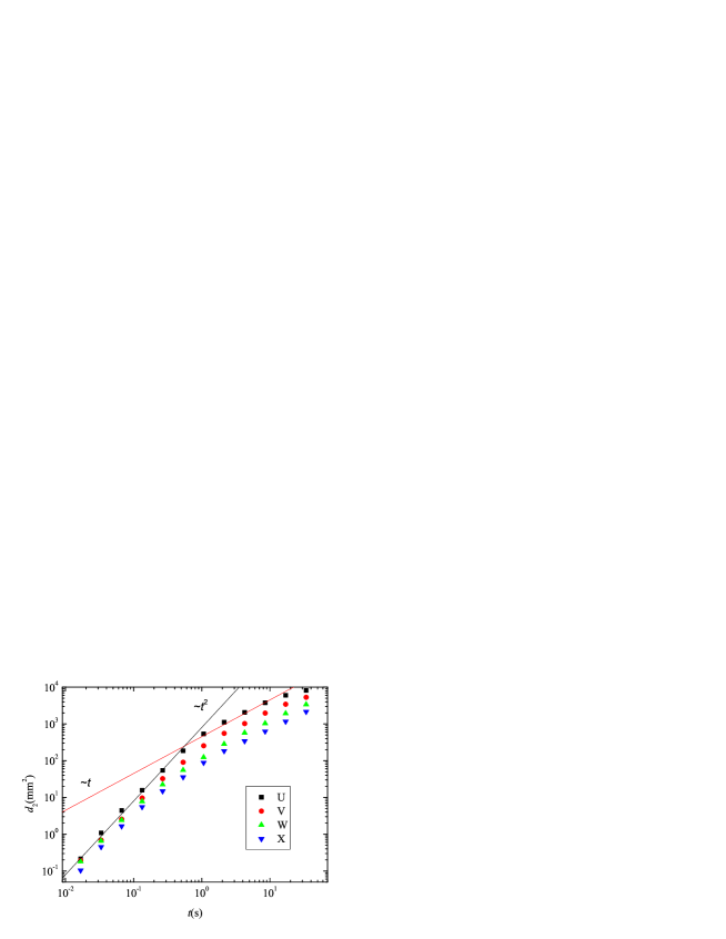
Figure 3: Mean squared displacement $d_{2}(t)$ for different packing fractions $\phi=10\%(\blacksquare),20\%(\bullet),30\%({\color[rgb]{0,1,0}\blacktriangle}),40\%({\color[rgb]{0,0,1}\blacktriangledown})$, with particles’ radius $\sigma=4$ mm and for driving with $f=200$ Hz (experiments with labels U,V,W,X). For all other parameters, see Table 1. Error bars fall within the symbols.

It is interesting to mention that the limit of the ballistic scale is mostly independent of the period of oscillation of the plate, even if it may be contrary to intuition. Our main interpretation of the motion of particles on the rough vibrating surface, discussed in Section IV.4, is that of a Brownian motion with viscous drag determining a characteristic relaxation time $\tau_{b}=1/\gamma_{b}$, basically related to the frictional properties of the sphere-surface contact, to which superimpose inelastic collisions with other particles occurring with a mean free time $\tau_{c}$. Such a model predicts a ballistic regime at times smaller than $\min[\tau_{c},\tau_{b}]$: quantitative assessment of $\tau_{b}$ and $\tau_{c}$ are well consistent with the estimate of $\Delta t_{diff}$ obtained here from the mean squared displacement (see discussion in Section V).

III Distributions of velocities

After a tiny transient regime, our system reaches a stationary homogeneous state, which is the subject of our research. Equilibrium statistical mechanics predicts a Gaussian (Maxwell-Boltzmann) distribution for velocities in a fluid. The deviation of velocities in granular fluids from the Maxwell-Boltzmann statistics is widely discussed in the literature van Noije and Ernst (1998); Puglisi et al. (1998); Losert et al. (1999). In the presence of uniform driving, however, those deviations are expected to be small and well reproduced by polynomial corrections superimposed to the usual Gaussian statistics.

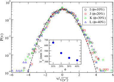
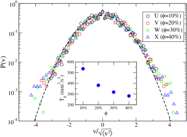
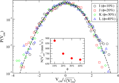
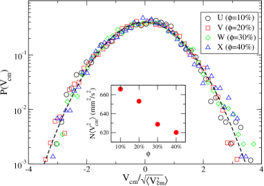
Figure 4: Top: particle velocity distributions (rescaled to have unit variance) for experiments with different packing fractions $\phi$ and particles of diameter $\sigma=1$ mm (left panels) and $\sigma=4$ mm (right panels), for driving with $f=200$ Hz. Bottom: center of mass velocity distributions for the same experiments, again rescaled to have unit variance. Dashed black lines are normalized Gaussian. For all other parameters, see Table 1. Insets: variances of the distributions, i.e. $T_{g}$ and $N\langle V_{cm}^{2}\rangle$, as functions of $\phi$.

In Fig. 4, two top frames, experimental rescaled velocity distributions are shown. Small but appreciable deviations from the Gaussian ideal curve are visible, mainly in the tails. Sonine-polynomial fits, not shown here, give a value for $a_{2}$ in the range $[0.01,0.05]$. The granular temperature $T_{g}=(1/2N)\sum_{i}{\bf v}_{i}^{2}$ is also shown in the insets: it decreases with the packing fraction $\phi$ as expected due to the increasing collision rate.

Notice that, as stated in the formula above, in the following we measure “temperatures” in units of squared velocities, i.e. ignoring the mass of the particle. Such a choice is possible because, here, temperature has only a kinetic meaning and does not correspond to environmental temperature (which occurs on energy scales exceedingly smaller).

III.1 Distribution of the center of mass velocity

In the two bottom frames of Fig. 4, one can see the distribution of one component ($x$ or $y$) of the center of mass velocity ${\bf V}_{cm}(t)=(1/N)\sum_{i=1}^{N}{\bf v}_{i}(t)$, collected over different configurations ($5\times 10^{3}$) in each experiment. It is interesting to notice how the distribution is well-fitted to a Gaussian. The rescaled variance $N\langle V^{2}_{cm}\rangle$ (where by isotropy we define $V_{cm}^{2}={\bf V}_{cm}^{2}/2$) is also plotted in the inset, as a function of the packing fraction. Notice that such a rescaled variance changes with the packing fraction on a much smaller energy interval with respect to the variation observed for $T_{g}$.

The effect of inter-particle collisions upon the center of mass velocity is much smaller when compared with the velocity of the single particle: indeed collisions conserve momentum for each component, so that the total momentum in a region is only affected by bounces on the plate, and by exchanges at the boundaries of the region as well (e.g. particles going in or out from the region itself). The latter contribution is as smaller as larger is the size of the region.

IV Structure factors

The main goal of our study is concerned with the characterization and the analysis of large-scale fluctuations. The physical quantities of interest are the correlations between the coarse-grained hydrodynamic fields, density $n({\bf r},t)$, velocity ${\bf u}({\bf r},t)$ and temperature $T({\bf r},t)$, defined as follows:

$$n({\bf r},t) = \sum_{i}\delta({\bf r}-{\bf r}_{i}(t)),$$

$${\bf u}({\bf r},t) = \frac{1}{n}\sum_{i}{\bf v}_{i}(t)\delta({\bf r}-{\bf r}_{i}(t)),$$ (1)

$$T({\bf r},t) = \frac{2m}{dn}\sum_{i}\frac{v^{2}_{i}(t)}{2}\delta({\bf r}-{\bf r}_{i}(t)),$$

where ${\bf r}_{i}(t)$ is the position of particle $i$ at time $t$, and the sum runs over the $N$ particles. In particular, we focus on large spatial scale fluctuations of the system around the stationary homogeneous state, where the hydrodynamic fields take the values $n=\overline{n}$, $T=\overline{T}$ and ${\bf u}=0$. We study fluctuations in momentum space and define $\delta{\bf a}({\bf k},t)=\{\delta n({\bf k},t),\delta T({\bf k},t),u_{\parallel}({\bf k},t),u_{\perp}({\bf k},t)\}$, with $\delta{\bf a}={\bf a}-{\bf\overline{a}}$, where the Fourier transform is

$$\delta{\bf a}({\bf k},t)=\int d{\bf r}~{}\delta{\bf a}({\bf r},t)e^{-i{\bf k}\cdot{\bf r}},$$ (2)

and $u_{\perp}({\bf k},t)$ and $u_{\parallel}({\bf k},t)$ denote the shear and longitudinal modes, respectively, namely

$$u_{\perp}({\bf k}) = \hat{k}_{\perp}\cdot{\bf u}({\bf k})$$

$$u_{\parallel}({\bf k}) = \hat{k}\cdot{\bf u}({\bf k}),$$ (3)

$\hat{k}_{\perp}$ being a unitary vector such that $\hat{k}_{\perp}\cdot\hat{k}=0$. In the following, we show and discuss the experimental data obtained for the static and dynamic correlation functions of the hydrodynamic fields, defined, in the stationary state, as

$$S_{ab}({\bf k})=\frac{1}{N}\langle\delta a({\bf k})\delta b({-\bf k})\rangle,$$ (4)

and

$$S_{ab}({\bf k},t)=\frac{1}{N}\langle\delta a({\bf k},t)\delta b({-\bf k},0)\rangle.$$ (5)

The study of these quantities provides important information on the structural properties of the system and on the characteristic lengths and times governing macroscopic fluctuations. In particular, at equilibrium and at small $k$, the static structure factors, Eq. (4), are related to thermodynamic quantities Hansen and McDonald (1996). From the measure of dynamic structure factors, Eq. (5), one can extract information on heat and sound hydrodynamic poles, and thus on the transport coefficients which rule thermal diffusion and propagation of pressure waves in the system.

From the procedural point of view, we measure structure factors $S_{ab}({\bf k},t)$ by directly applying definitions (2)-(5) on a set of wave-vectors ${\bf k}$, averaging over several (typically $5\times 10^{3}$) configurations; subsequently, we compute sphericized averages $S_{ab}(k,t)$ over shells with average modulus $k$, assuming isotropy. The smallest value of $k$ considered is $k_{min}=2\pi/(D/2)$ accordingly to the largest linear size of the system (we recall that $D$ is the diameter of the container). In the case where we focus on the central region of width $L_{x}=D/2$, the minimum value of wave-vector is $k_{min}=2\pi/(L_{x}/2)$. For the largest value of $k$ we have chosen a value, typically smaller than the diameter of the particles, convenient with respect to the relevant information we want to highlight (e.g. for the velocity structure factor it is useful to give a convincing evidence of the reached “plateau” at large $k$).

IV.1 Density structure factor

From Eq. (4) we get the density structure factor

$$S_{nn}({\bf k})=\frac{1}{N}\langle\delta n({\bf k})\delta n({-\bf k})\rangle=\frac{1}{N}\left\langle\sum_{i,j=1}^{N}\exp(-i{\mathbf{k}}\cdot({\mathbf{r}}_{i}-{\mathbf{r}}_{j}))\right\rangle,$$ (6)

where the average is taken over the stationary state.

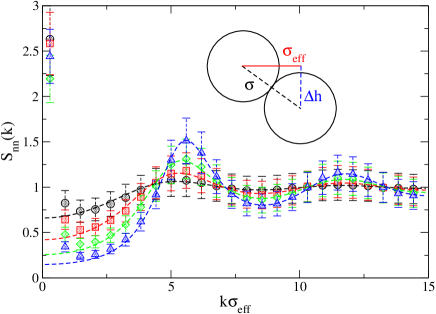
Figure 5: Density structure factors at various packing fractions $\phi$ for particles with diameter $\sigma=4$ mm and for driving with $f=200$ Hz (experiments U,V,W,X). The dashed lines represent the analytical prediction for elastic hard disks Baus and Colot (1986). In the graph on the left the experimental results are plotted versus $k\sigma$, while in the graph on the right they are shown versus $k\sigma_{eff}$ with $\sigma_{eff}/\sigma=cos(\pi/6)$. The cartoon in the second graph illustrates the meaning of $\sigma_{eff}$ which is the effective diameter seen by particles which collide at an average height $\approx\sigma/2$. For all experimental parameters, see Table 1.

In Fig. 5 we show $S_{nn}(k)$ measured in our system, together with the analytical prediction for an elastic system of hard discs. The comparison with the elastic system shows two main differences. First, at small $k$ the structure factors displays an enhancement, signalling long range density correlations due to inelasticity. Those correlations are not the main objective of our analysis here and have been addressed before, see for instance Olafsen and Urbach (1998); Cecconi et al. (2004); Bordallo-Favela et al. (2009). Notice that such correlations at large wavelengths do not depend monotonously on $\phi$: higher packing fractions, as a matter of fact, enhance both the aggregating role of dissipation (due to inelastic collisions) and the dispersive role of excluded volume. Therefore, they may have negative or positive influence on the density structure. Second, at larger $k$ the theoretical curves for elastic hard discs are in excellent agreement with our experiment, when the abscissa is rescaled by a factor $\cos(\pi/6)$, as shown in the right frame of Fig. 5. Such a rescaling is equivalent to consider an effective diameter of particles $\sigma_{eff}\approx\cos(\pi/6)\sigma$. Indeed, particles typically collide at different heights from the plate and therefore meet at a distance smaller than their diameter. Such an observation is consistent with an average difference of height $\Delta h\approx\sigma/2$.

IV.2 Transverse velocity modes

As discussed below, in the realm of linear hydrodynamics, transverse velocity modes are decoupled from the other hydrodynamic fields and their behaviour can be studied separately. From Eq. (4) one has

$$S_{\perp}({\bf k})=\frac{1}{N}\langle u_{\perp}({\bf k})u_{\perp}({-\bf k})\rangle.$$ (7)

In Fig. 6, $S_{\perp}(k)$ is reported for different values of $\phi$, at fixed amplitude and frequency of oscillation. In all cases, we find two plateau, at large and small $k$. The former coincides with the granular temperature $T_{g}$ of the system and is determined by the packing fraction. The latter is much less dependent on $\phi$ and is approximately constant within experimental errors. Its value is expected to be mostly related to the energy injection mechanism, namely to the shaking parameters. Indeed, in Figs. 7 and 8 the structure factor of transverse modes is shown upon varying the frequency and amplitude of oscillation, respectively, keeping fixed the packing fraction. In these cases a strong dependence of $S_{\perp}(k)$ at small $k$ on these parameters is observed. At small $k$ we have also reported (see dashed lines) the values of $N\langle V_{cm}^{2}\rangle$, whose relevance at large scales is discussed below.

The main feature arising from the figures illustrated above is a “sigmoidal” shape of the structure factor that can be clearly observed in the whole range of parameters. Note that we have intentionally avoided a too high resolution in $k$, to neglect “fine” effects which have a less clear interpretation: for instance, it would be interesting but beyond the scope of our analysis here, to give an interpretation of the oscillations at large k that can be observed with a higher $k$-resolution, see Fig. 9 for an example. The main “sigmoidal” shape is remarkably different from what is observed in elastic fluids, where static velocity structure factors are flat. The profile we observe connects two regions in $k$ space with different energy scales: one associated with the granular temperature and the other one related to the external driving mechanism. As it will be thoroughly discussed below, this behavior suggests the existence of a characteristic length-scale in the system, marking the passage from one region to the other.

In order to study the characteristic times in our system, we have also measured the dynamic structure factor

$$S_{\perp}({\bf k},t)=\frac{1}{N}\langle u_{\perp}({\bf k},t)u_{\perp}({-\bf k},0)\rangle,$$ (8)

that is reported in Fig. 10, for different values of the experimental parameters. Notice that, at small $k$, the decay in time of $S_{\perp}(k,t)$ is nearly exponential. Moreover, the decorrelation time is greater for smaller $k$. A more detailed analysis of such behavior is postponed to Section V.

In Fig. 11 the probability distribution functions (rescaled to have unitary variance) of the transverse velocity modes are shown. For different values of the parameters, we always observe Gaussian distributions.

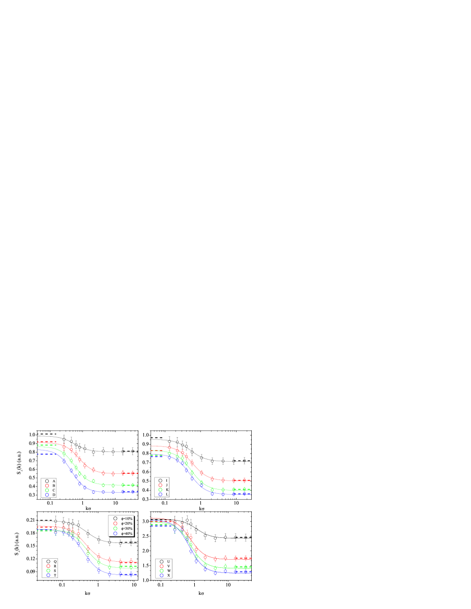
Figure 6: Transverse velocity structure factors at various $\phi$ (see the legend), with particles’ diameters $\sigma=2$ mm (top left), $\sigma=1$ mm (top right and bottom left) and $\sigma=4$ mm (bottom right), for regions of interest “center” (top panels) and “whole” (bottom panels), and driving with $f=200$ Hz. For all experimental parameters, see Table 1. Dashed lines mark the value of $N\langle V_{cm}^{2}\rangle$ and $T_{g}$ at low and large values of $k$ respectively. The continuous curves are fits with formula (16).

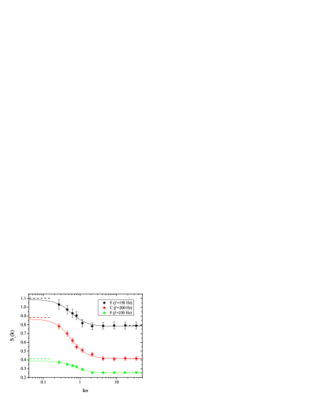
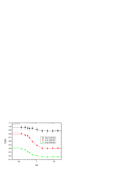
Figure 7: Transverse velocity structure factors at various frequencies $f$ and fixed packing fraction $\phi=30\%$ and acceleration, with particles’ diameter $\sigma=2$ mm (left panel) and $\sigma=1$ mm (right panel). For all other experimental parameters, see Table 1. Dashed lines mark the value of $N\langle V_{cm}^{2}\rangle$ and $T_{g}$ at low and large values of $k$ respectively. The continuous curves are fits with formula (16).

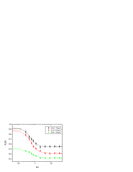
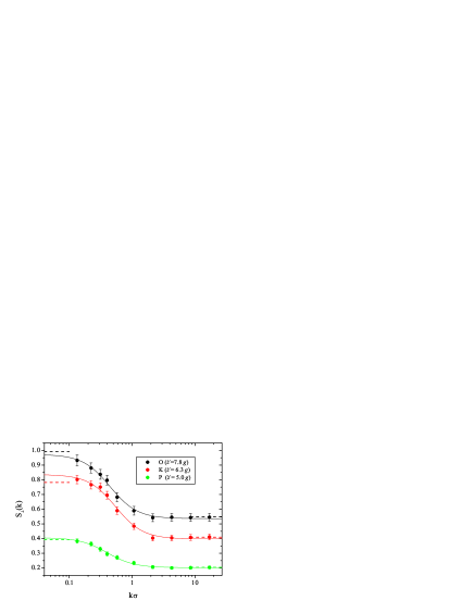
Figure 8: Transverse velocity structure factors at various maximum acceleration of the plate $\ddot{z}_{max}$ and constant frequency $f=200$ Hz, at packing fraction $\phi=30\%$ and with particles’ diameter $\sigma=2$ mm (left panel) and $\sigma=1$ mm (right panel). For all other experimental parameters, see Table 1. Dashed lines mark the value of $N\langle V_{cm}^{2}\rangle$ and $T_{g}$ at low and large values of $k$ respectively. The continuous curves are fits with formula (16).

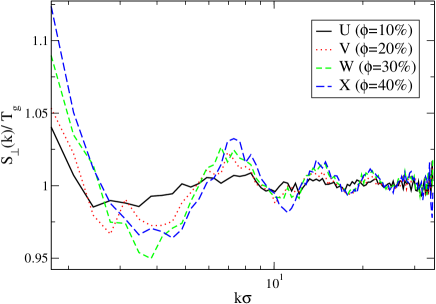
Figure 9: Transverse velocity structure factors, rescaled by $T_{g}$, at various packing fractions with particles’ diameter $\sigma=4$ mm and for driving with $f=200$ Hz (experiments with labels I, J, K, and L), at high values of $k$ and finer $k$-resolution, in order to show the oscillations, which are similar to the ones observed in the density structure factor. For all experimental parameters, see Table 1.

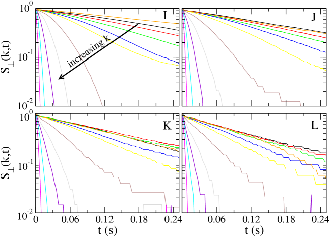
Figure 10: Temporal decay of the transverse velocity modes, $S_{\perp}(k,t)$, rescaled by its value at time $t=0$, in experiments with different packing fractions $\phi=10\%$ (I), $\phi=20\%$ (J), $\phi=30\%$ (K) and $\phi=40\%$ (L), with particles’ diameter $\sigma=1$ mm and for driving with $f=200$ Hz. For all other experimental parameters, see Table 1. The values of $k\sigma$ are the following: $0.089$, $0.14$, $0.2$, $0.26$, $0.32$, $0.51$, $1$, $2$, $4$, $8$, $16$. Error bars are omitted to improve legibility.

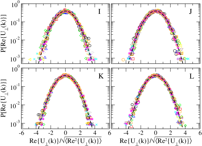
Figure 11: Probability density functions of transverse velocity modes (real part), rescaled to have unit variance, for experiments with different packing fractions $\phi=10\%$ (I), $\phi=20\%$ (J), $\phi=30\%$ (K) and $\phi=40\%$ (L), with particles’ diameter $\sigma=1$ mm and for driving with $f=200$ Hz. For all other experimental parameters, see Table 1. The values of $k\sigma$ are the following: $0.089$, $0.14$, $0.2$, $0.26$, $0.32$, $0.51$, $1$, $2$, $4$, $8$, $16$.

IV.3 Longitudinal velocity modes

The structure factor of longitudinal velocity modes

$$S_{\parallel}({\bf k})=\frac{1}{N}\langle u_{\parallel}({\bf k})u_{\parallel}({-\bf k})\rangle$$ (9)

is shown in Fig. 12, for different values of the experimental parameters (see caption). The same qualitative behaviour is observed as for transverse modes: two energy scales are present at large and small $k$, representing the granular temperature and the energy scale associated to the fluctuations of the center-of-mass velocity, respectively. Again, a characteristic length scale can be associated with the spatial correlation of longitudinal modes, as discussed in more detail below.

The temporal decay of time correlations of longitudinal modes $S_{\parallel}({\bf k},t)=\frac{1}{N}\langle u_{\parallel}({\bf k},t)u_{\parallel}({-\bf k},0)\rangle$, is shown in Fig. 13. Here we find a behaviour much more complex than a simple exponential decay. This is due to the coupling of the longitudinal modes with the other hydrodynamic fields.

Finally, in Fig. 14 the probability distribution functions of $u_{\parallel}({\bf k})$ are reported. Again, we find that such distributions are nearly Gaussian.

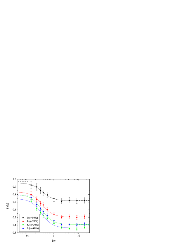
Figure 12: Longitudinal velocity structure factors at various $\phi$ (experiments with labels I, J, K and L). For all experimental parameters, see Table 1. Dashed lines mark the value of $N\langle V_{cm}^{2}\rangle$ and $T_{g}$ at low and large values of $k$ respectively. The continuous curves are fits with formula (20).

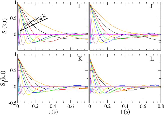
Figure 13: Temporal decay of the longitudinal velocity modes, $S_{\parallel}(k,t)$, rescaled by its value at time $t=0$, in experiments with different packing fractions $\phi=10\%$ (I), $\phi=20\%$ (J), $\phi=30\%$ (K) and $\phi=40\%$ (L), with particles’ diameter $\sigma=1$ mm and for driving with $f=200$ Hz. For all other experimental parameters, see Table 1. The values of $k\sigma$ are the following: $0.089$, $0.14$, $0.2$, $0.26$, $0.32$, $0.51$, $1$, $2$, $4$, $8$, $16$. Error bars are omitted to improve legibility.

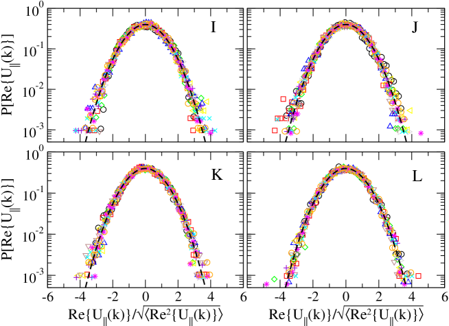
Figure 14: Probability density functions of longitudinal velocity modes (real part), rescaled to have unit variance, for experiments with different packing fractions $\phi=10\%$ (I), $\phi=20\%$ (J), $\phi=30\%$ (K) and $\phi=40\%$ (L), with particles’ diameter $\sigma=1$ mm and for driving with $f=200$ Hz. For all other experimental parameters, see Table 1. The values of $k\sigma$ are the following: $0.089$, $0.14$, $0.2$, $0.26$, $0.32$, $0.51$, $1$, $2$, $4$, $8$, $16$.

IV.4 Comparison with theory and simulations: “bath temperature” and correlation lengths

In order to discuss a theoretical model for our system, we show, starting from the definition of $S_{\perp}(k)$, see Eq. (7), what the physical meaning of the two plateau appearing in Fig. 6 is. At large values of $k$ in Eq. (7) only the diagonal term survives:

$$S_{\perp}(k)\rightarrow\langle\frac{1}{N}\sum_{i}\frac{{\bf v}_{i}^{2}}{2}\rangle=T_{g},$$ (10)

whereas at small values of $k$ we have

$$S_{\perp}(k\to 0)=\frac{N}{2}\langle\left(\frac{1}{N}\sum_{i}{\bf v_{i}}\right)^{2}\rangle=\frac{N}{2}\langle{\bf V}_{cm}^{2}\rangle\equiv N\langle V_{cm}^{2}\rangle.$$ (11)

For large values of $k$ the velocity structure factor is proportional to the average square velocity of particles, i.e. $T_{g}$, while at small $k$ values one has $S_{\perp}(k)=N\langle{\bf V}_{cm}^{2}\rangle$, with ${\bf V}_{cm}$ almost independent of (momentum conserving) collisions and affected only by the interaction with the vibrating plate. Let us note that, since in our system the momentum is not conserved, we have that the value of $S_{\perp}(k=0)$ is not constrained to a $\delta(k)$ and can be compared to the values of the function in the neighbourhood of $k=0$.

A model theory that fully accounts for the dissipative interactions among hard particles and between particles and the vibrating vessel is beyond our scope Brey et al. (1998, 2009); Maynar et al. (2009). We are interested into an effective model that can reproduce the behavior of collective modes at large length scales.

For instance, let us consider the shear modes, which, according to linear hydrodynamic theory, are decoupled from the other modes of the system Hansen and McDonald (1996). The presence of an exponential decay for $\langle u_{\perp}({\bf k},t)u_{\perp}(-{\bf k},0)\rangle$, which can be seen in the panels of Fig. 10, and the measure of a Gaussian distribution for the real (and imaginary) part of the variable $u_{\perp}(k)$, see Fig. 11, suggest that the dynamics of $u_{\perp}(k)$ is ruled by a simple linear Langevin equation. Similarly, for the longitudinal modes $u_{\parallel}(k)$ a Gaussian distribution for the real (and imaginary) part is found, as shown in Fig. 14, while the decay in time presents an exponentially damped oscillation. This behaviour is consistent, as discussed below, with a linear system of Langevin equations which couples longitudinal modes to temperature and density modulations, as dictated by linear hydrodynamics.

One of the central points to be addressed in order to give a theoretical description of our system is the energy injection mechanism. Indeed, in a system of particles with dissipative interactions, the collective behaviour strongly depends on the kind of energy injection, as it is clear comparing, for instance, the low $k$ tails of velocity structure factors in Refs.Gradenigo et al. (2011b); van Noije et al. (1999), where different kinds of model thermostats are studied. In particular, we assume that the velocity of the $i$-th particle ${\bf v}_{i}$ of our experiment evolves in time according to the stochastic equation:

$$\dot{{\bf v}}_{i}(t)=-\gamma_{b}{\bf v}_{i}(t)+\boldsymbol{\zeta}_{i}(t)+{\bf F}_{i}(t),$$ (12)

where the force ${\bf F}_{i}(t)$ accounts for the inelastic collisions with other particles and we assume that the interaction between the vibrating vessel and each particle can be modeled as an equilibrium thermostat with a viscous drag $-\gamma_{b}{\bf v}_{i}(t)$ and a white noise $\boldsymbol{\zeta}_{i}$ satisfying the 2nd kind FDT, namely we assume for the noise: $\langle\boldsymbol{\zeta}_{i}(t)\boldsymbol{\zeta}_{j}(t^{\prime})\rangle=2\gamma_{b}T_{b}\delta(t-t^{\prime})\delta_{i,j}$, with $\gamma_{b}$ the friction coefficient. According to this model, the energy of the center of mass of the system and the low $k$ value of $S_{\perp}(k)$ are related to the temperature of the thermostat:

$$S_{\perp}(k)\to N\langle V_{cm}^{2}\rangle=T_{b}.$$ (13)

To explain the shape of the structure factors, a theory for macroscopic fields has to be developed from the microscopic equation (12). Hydrodynamics is the proper candidate when separation of scales exists between “fast” relaxing microscopic modes and “slow” relaxating macroscopic ones, a condition always to be verified in granular fluids Goldhirsch (1999); Kadanoff (1999), but well satisfied in our experiment. Fluctuating hydrodynamics is a correction to such a theory when macroscopic scales are not large enough to neglect fluctuations. A more detailed derivation of the stochastic equations for the hydrodynamic fields starting from microscopic dynamics can be found in Gradenigo et al. (2011b). Here, we just provide phenomenological arguments for the Langevin equation that governs the shear modes. According to the observation of two relevant energy scales in our system, we assume two sources of hydrodynamic noise of different amplitude: an internal one, $\eta_{I}(k,t)$, due to the collisions between particles, and an external one, $\eta_{E}(k,t)$, due to the action of the external thermostat. These noises have zero average and variance:

$$\langle\eta_{I}(k,t)\eta_{I}(k^{\prime},t^{\prime})\rangle=2T_{g}\nu k^{2}\delta(t-t^{\prime})\delta(k+k^{\prime})$$

$$\langle\eta_{E}(k,t)\eta_{E}(k^{\prime},t^{\prime})\rangle=2\gamma_{b}T_{b}\delta(t-t^{\prime})\delta(k+k^{\prime})$$

$$\langle\eta_{E}(k,t)\eta_{I}(k^{\prime},t^{\prime})\rangle=0,$$ (14)

where $\nu$ is the kinematic viscosity. Then, in agreement with a 2nd kind FDT principle, we introduce a frictional term proportional to each source of randomness, obtaining the following Langevin equation:

$$\dot{u}_{\perp}(k,t)=-(\gamma_{b}+\nu k^{2})u_{\perp}(k,t)+\eta_{I}(k,t)+\eta_{E}(k,t).$$ (15)

Such an equation accounts for all the experimental observations on shear modes presented above, namely the exponential decay of the time autocorrelation, the Gaussian distribution of $\textrm{Re}[u_{\perp}(k,t)]$ (and its imaginary part), and in particular the shape of the structure factor. We can say that each mode is at equilibrium, but with a different temperature. The system as a whole is of course out of equilibrium as long as $T_{g}\neq T_{b}$. Such an observation gives us the way to discuss one of the most intriguing feature of the non-equilibrium structure of velocity correlations, namely the finding of a correlation length not present at equilibrium. Indeed, the temperature spectrum of modes, which is nothing but the velocity structure factor, can be obtained from Eq. (15) and reads as

$$S_{\perp}(k)=N^{-1}\langle|u_{\perp}(k)|^{2}\rangle=\frac{\gamma_{b}T_{b}+\nu k^{2}T_{g}}{\gamma_{b}+\nu k^{2}}=T_{g}+\frac{T_{b}-T_{g}}{1+\xi_{\perp}^{2}k^{2}},$$ (16)

which defines the correlation length for transverse modes

$$\xi_{\perp}=\sqrt{\nu/\gamma_{b}}.$$ (17)

At equilibrium, namely when collisions are elastic and $T_{g}=T_{b}$, the equipartition between modes is perfectly fulfilled and the structure factor becomes flat, i.e. we have a single temperature for all the modes: $S_{\perp}(k)=T_{b}$. Differently, in our non-equilibrium system of interest, where $T_{g}\neq T_{b}$, equipartition is broken and we find an explicit dependence of $S_{\perp}(k)$ on $k$. Performing the 2D inverse Fourier transform $\mathcal{T}^{-1}$, in real space Eq. (16) acquires a plain meaning:

$$\mathcal{T}^{-1}S_{\perp}=T_{g}\delta^{(2)}({\bf r})+(T_{b}-T_{g})\frac{K_{0}(r/\xi_{\perp})}{\xi_{\perp}^{2}},$$ (18)

where $K_{0}(x)$ is the 2nd kind modified Bessel function that, for large distances, decays exponentially

$$K_{0}(r/\xi_{\perp})\approx\sqrt{\frac{\pi}{2}}\frac{e^{-r/\xi_{\perp}}}{(r/\xi_{\perp})^{1/2}}.$$ (19)

The existence of two different and well defined energy scales has a neat consequence both in real and in Fourier space. In real space the distance from equilibrium $T_{b}-T_{g}$ determines the amplitude of non equilibrium correlations in the velocity field, see Eq. (18). In Fourier space a division in two subsystems that respectively equilibrated at high or low temperature takes place. By looking at Fig. 6 we may identify the characteristic momentum $k^{*}$ corresponding to the characteristic length $\xi_{\perp}$ as the conventional point which separates the subset of “hot” modes from the subset of “cold” modes.

For the interested reader, a comprehensive discussion on the relations between noises, covariances and large scale correlations for the model (12) is addressed in Gradenigo et al. (2011b). Clearly, the linearization of hydrodynamic equations is only possible in a certain range of densities, and, in particular, when the granular fluid becomes too dense, new couplings appear and non-linear effects become relevant. For instance, at packing fractions where a glassy-like arrest of dynamics occurs Keys et al. (2007b); Kranz et al. (2010), the linearized hydrodynamics is no more expected to be effective. For the longitudinal velocity modes, we find an exponentially damped oscillating function. This is consistent with the fact that even within linear hydrodynamics they are coupled to temperature and density fluctuations and hence their temporal decay has more than one characteristic time-scale. Their frequency power spectrum $S_{\parallel}(k,\omega)$ has been calculated analytically for the same energy injection mechanism of Eq. (12) in Gradenigo et al. (2011b). Relying on the fluctuating hydrodynamic equations, the static longitudinal velocity correlator turns out to be well approximated at low $k$ values by the functional form:

$$S_{\parallel}(k)=T_{b}-(T_{b}-T_{g})\xi_{\parallel}^{2}k^{2}+\mathcal{O}(k^{4})=T_{g}+\frac{T_{b}-T_{g}}{1+\xi_{\parallel}^{2}k^{2}}+\mathcal{O}(k^{4}),$$ (20)

where $\xi_{\parallel}$ does not depend only on the drag coefficient $\gamma_{b}$ of the thermal bath and on the longitudinal viscosity $\nu_{l}$ but also on other microscopic parameters, as reported explicitly in Gradenigo et al. (2011b). As can be seen from Fig. 12, the sigmoidal shape of $S_{\parallel}(k)$ obtained from Eq. (20) is in good agreement with experiments. The fact that the low momentum approximation of $S_{\parallel}(k)$ recovers also the large $k$ asymptote is not surprising: $S_{\parallel}(k)$ represents the power spectrum of a projection of the velocity field and is therefore strictly bounded by the energy scales dominant al large and small $k$.

V Time-scales, temperatures and correlation lengths

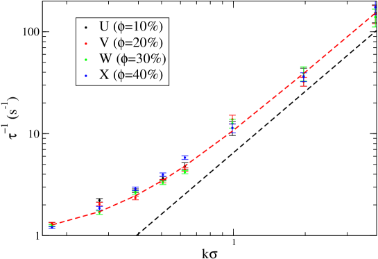
Figure 15: Slopes of exponential decays at different values of $k$ for $S_{\perp}(k,t)$ in experiments with different packing fractions $\phi=10\%$ (U), $\phi=20\%$ (V), $\phi=30\%$ (W) and $\phi=40\%$ (X), with particles’ diameter $\sigma=4$ mm and for driving with $f=200$ Hz. For all other experimental parameters, see Table 1.

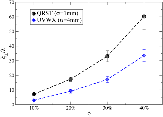
Figure 16: Correlation lengths $\xi_{\perp}$ rescaled by the mean free path $\lambda$ as function of the packing fraction $\phi$, for the transverse velocity fields for different groups of experiments, with labels Q, R, S and T (diameter $\sigma=1$ mm) and with labels U, V, W and X (diameter $\sigma=4$ mm), for driving with $f=200$ Hz. The method of computing $\xi_{\perp}$ is discussed in Sec. V. For all other experimental parameters, see Table 1.

From Eq. (15) the theoretical prediction for the time autocorrelation is

$$S_{\perp}(k,t) \sim\exp(-t/\tau(k))$$ (21)

$$\tau(k)^{-1} =\gamma_{b}+\nu k^{2}.$$ (22)

The decay in time of $S_{\perp}(k,t)$, as reported for instance in Fig. 10, can be fit by exponentials, accepting a relative error in the order of $5\div 10\%$ after a least squares procedure. For a few experiments we have analyzed the results of such fits, finding good agreement with the parabolic behaviour, see Fig. 15. From the parabolic fit we extract both the kinematic viscosity $\nu$ and the drag coefficient of the vibrating vessel $\gamma_{b}$ and obtain the length-scale $\xi_{\perp}$ at various packing fraction. Those values, for some of the experiments, are reported in Table 2.

$\phi$	$\gamma_{b}$(s-1)	$\nu_{\perp}$(mm2/s)	$\xi_{\perp}$(mm)
10%	$1.1\pm 0.1$	$170\pm 20$	$11.8\pm 2$
20%	$1.1\pm 0.1$	$145\pm 20$	$11.5\pm 2$
30%	$0.97\pm 0.1$	$156\pm 20$	$12.5\pm 2$
40%	$0.96\pm 0.1$	$145\pm 20$	$12.3\pm 2$

Table 2: $\gamma_{b}$, $\nu_{\perp}$ and $\xi_{\perp}$ as measured from exponential decays, formula (22), in experiments with particles’ diameter $\sigma=4$ mm, for driving with $f=200$ Hz and all the other parameters are fixed to the values corresponding to label U of Table 1. In particular, the dependence of $\xi_{\perp}/\lambda$ on $\phi$ is shown in Fig. 16.

Both $\gamma_{b}$ and $\nu_{\perp}$ remain roughly constant when the packing fraction is varied from $10\%$ to $40\%$. A constant value for $\gamma_{b}$ is in fair agreement with the interpretation that it represents an effective viscous drag of the particle-plate interaction, as it appears in the microscopic “thermostatted” model, Eq. (12). The kinematic viscosity, on the other side, could weakly depend on $\phi$, as well as on the internal temperature $T_{g}$, but variations of those parameters are not large enough to result in appreciable variations of $\nu_{\perp}$. Estimates, expected to be reliable in the dilute limit, give $\nu_{\perp}\sim T_{g}\tau_{c}$ where $\tau_{c}$ is the mean free time between collisions: the comparison with the values of $T_{g}$ (reported below) is compatible with a mean free time $\tau_{c}\sim 0.1\div 0.5$ seconds, which, in turn, agrees with the typical crossover time from ballistic to diffusive behavior, see Fig. 3. It is also important to notice that the order of magnitude of time-scale separation between the single particle relaxation $\gamma_{b}$ and the collective (collisional) relaxation $\tau_{c}$ is $\tau_{c}\gamma_{b}\sim 0.1\div 0.5$: this is reflected in a not very large difference between $T_{b}$ (or its estimate $N\langle V_{cm}^{2}\rangle$) and $T_{g}$. Such lack of good separation of scales makes difficult to use linearized hydrodynamics for quantitative predictions of velocity correlations: its predictive power is fully appreciated only when time-scales are well separated, as it happens with numerical simulations Gradenigo et al. (2011b, a). Here, the fits of structure factor data realized with formula (16) and shown in Figures 6, 7, 8 and 12, lead to estimates of the physical parameters not always consistent with those obtained independently (e.g. in the procedure discussed above for $\gamma_{b}$ and $\nu_{\perp}$). For this reason in the following we have used more rough estimates of the main observables when comparing different experiments, as it is done in Table  3.

Label	$\phi$	$T_{g}$	$N\langle V_{cm}^{2}\rangle\approx T_{b}$	$\xi_{\perp}$	$\xi_{\parallel}$	$\xi_{\perp}/\lambda$	$\xi_{\parallel}/\lambda$
		(mm2/s2)	(mm2/s2)	mm	mm
A	10%	730	910	19	21	5	5
B	20%	499	829	15	20	10	13
C	30%	373	794	19	21	22	25
D	40%	306	699	20	20	42	41
E	30%	713	993	17	19	20	23
F	30%	231	371	14	18	17	22
G	30%	499	822	20	19	24	23
H	30%	289	462	17	18	20	22
I	10%	650	876	11	16	6	8
J	20%	457	749	10	15	13	19
K	30%	368	704	11	17	27	40
L	40%	324	691	12	17	50	71
M	30%	796	959	7	16	17	39
N	30%	160	370	15	17	37	42
O	30%	492	892	13	17	31	40
P	30%	183	355	15	14	36	35
Q	10%	600	794	13	19	7	10
R	20%	421	733	14	12	17	16
S	30%	389	701	14	21	33	50
T	40%	316	711	15	5	60	23
U	10%	536	666	22	32	3	4
V	20%	381	653	28	33	9	11
W	30%	318	629	29	34	17	20
X	40%	282	620	32	32	33	33

Table 3: Temperatures and correlation lengths measured in the experiments, following the phenomenological interpretation given in Section IV.4. Lengths are measured in millimeters, time is measured in seconds.

The values for the correlation lengths are simply obtained by interpolating the wavelength where the structure factors cross half of their way between their maximum and minimum value, i.e. $\xi_{\perp}=2\pi/k^{*}$ and $S_{\perp}(k^{*})\approx\frac{S_{\perp}(k\to 0)+S_{\perp}(k\to\infty)}{2}$, and analogously for $\xi_{\parallel}$. Such a definition does not coincide in absolute value with that, coming from the theoretical model, $\xi_{\perp}\sim\sqrt{\nu/\gamma_{b}}$ : indeed the latter is smaller of about a factor $3$ (compare Table 2 with Table 3, last four lines). Nevertheless, when comparing the same protocol of measurement in different experimental conditions, we expect the choice of protocol to be not too relevant.

The granular temperatures $T_{g}$ are compatible with thermal velocities $\sqrt{T_{g}}$ which are about $1/5\div 1/10$ of the maximum vertical velocity of the plate, independently of the mass of the particles. Fluctuations of center of mass velocity, $N\langle V_{cm}^{2}\rangle$, remain more stable than $T_{g}$ when the packing fraction is changed, while they do show clear variations when the shaking parameters are modified: this behavior is in good agreement with the interpretation of such a quantity as the estimate of the “bath temperature” $T_{b}$. Apparently, changing the vibration frequency (at constant acceleration) has a more deep effect on $T_{b}$ with respect to a variation of the acceleration at constant frequency (compare experiments E-F vs G-H, using C as a reference, as well as experiments M-N vs O-P, using K as a reference).

A general comment concerns the fact that the best agreement with the phenomenological fluctuating hydrodynamic model is achieved for the experiments with the fully photographed system (i.e. without excluding the border regions), experiments from $Q$ to $X$. In those cases, indeed, one can reach smaller values of $k$ both in comparison with the mean free path $\lambda$ and with the correlation lengths. Moreover, in this case the estimate of $T_{b}$ through $N\langle V_{cm}^{2}\rangle$ is more reliable because the system under observation is really closed, i.e. center of mass fluctuations are not influenced by collisions of particles inside the system with particles outside the system.

The correlation lengths separating the “cold” (inelastic) scales from the “hot” (elastic) ones, do not change appreciably as the packing fraction is changed and all other parameters are fixed, but they display a pronounced increase with the packing fraction when normalized by the mean free path, as can be clearly seen in Fig. 16. The meaning of such an observation is that the number of collisions between correlated particles increases with the occupied volume. The longitudinal correlation length $\xi_{\parallel}$ is – on average – slightly larger than the transveral one $\xi_{\perp}$, as expected also from a more detailed analysis of fluctuating hydrodynamics Gradenigo et al. (2011b).

VI Conclusions

We have reported experiments on the measurements of density and velocity structure factors in a homogeneously driven quasi-2D granular material. We compared the results with a recent fluctuating hydrodynamic theory derived from a thermostatted microscopic model Gradenigo et al. (2011b). To the best of our knowledge, together with a previous publication which included some of the results presented here Gradenigo et al. (2011a), this is the first systematic comparison between a granular experiment and granular fluctuating hydrodynamics. Considering the approximations involved in the theory, it is remarkable to observe agreements in so many aspects: 1) the basic shape of the velocity structure factors, which interpolates between a “high energy” plateau at small $k$ and a “low energy” plateau at large $k$; 2) the decay of autocorrelation of velocity modes, which is roughly exponential for transverse modes and damped oscillating for the longitudinal ones; 3) the Gaussian character of all fluctuations of modes; 4) the closeness of the high energy plateau to the variance of the fluctuations of the center of mass velocity; 5) the fact that such a plateau strongly depends on the shaking parameters and much more weakly on the packing fraction.

There are two basic assumptions underlying the theory, which are indirectly confirmed by the good agreement between the experiment and the predictions of the theory: 1) a microscopic model which includes a “thermostat” with temperature $T_{b}$ and viscous drag $\gamma_{b}$; 2) a sufficient separation of scales such that external noise (from the thermostat) and internal one (from collisions) are separated and the latter is well reproduced by a “local equilibrium” assumption de Zarate and Sengers (2006). The “bath temperature” $T_{b}$ , indeed, seems to be well measured in the experiment by evaluating the high energy plateau of the velocity structure factors (at low $k$) or the variance of the fluctuations of the center of mass velocity multiplied by $N$. However, the separation of scales is not significant enough to get a perfect comparison for the complete structure factors (e.g. with formula (16) or (20)). The theory allows us to define and measure a non-equilibrium correlation length as well, which increases (in terms of particle mean free paths) when the packing fraction is increased, representing the separation of ordered “cold” scales and more disordered “hot” scales which are in equilibrium with the bath.

Future investigations including a more detailed study of the vertical-to-horizontal energy transfer mechanism are in progress, with the aim of achieving a predictive theory for the properties of the effective bath $T_{b}$ and $\gamma_{b}$ as functions of the shaking parameters and the frictional properties of the surface.