3D simulations of microquasar jets in clumpy stellar winds

Abstract

Context. High-mass microquasars consist of a massive star and a compact object, the latter producing jets that will interact with the stellar wind. The evolution of the jets, and ultimately their radiative outcome, could depend strongly on the inhomogeneity of the wind, which calls for a detailed study.

Aims. The hydrodynamics of the interaction between a jet and a clumpy wind is studied, focusing on the global wind- and single clump-jet interplay.

Methods. We have performed, using the code Ratpenat, three-dimensional numerical simulations of a clumpy wind interacting with a mildly relativistic jet, and of individual clumps penetrating into a jet.

Results. For typical wind and jet velocities, filling factors of about $\ga 0.1$ are already enough for the wind to be considered as clumpy. An inhomogeneous wind makes the jet more unstable when crossing the system. Kinetic luminosities $\sim 10^{37}$ erg/s allow the jet to reach the borders of a compact binary with an O star, as in the smooth wind case, although with a substantially higher degree of disruption. When able to enter into the jet, clumps are compressed and heated during a time of about their size divided by the sound speed in the shocked clump. Then, clumps quickly disrupt, mass-loading and slowing down the jet.

Conclusions. We conclude that moderate wind clumpiness makes already a strong difference with the homogeneous wind case, enhancing jet disruption, mass-loading, bending, and likely energy dissipation in the form of emission. All this can have observational consequences at high-energies and also in the large scale radio jets.

1 Introduction

Microquasars are binary systems hosting a star and an accreting black hole or neutron star. Matter from the star is transferred to the compact object, part of it being launched through magnetocentrifugal forces (e.g., Blandford & Znajek, 1977; Blandford & Payne, 1982; Barkov & Khangulyan, 2011). This triggers the formation of bi-polar jets, which generate non-thermal radio emission (e.g., Mirabel et al., 1999; Ribó, 2005), and are thought to be the location from where the gamma rays observed in some sources are emitted (e.g., Albert et al., 2007; Tavani et al., 2009; Abdo et al., 2009; Sabatini et al., 2010). Jets could be magnetically dominated at their base, but magnetohydrodynamical processes occurring at higher jet height would accelerate the flow, efficiently converting magnetic energy into kinetic one (e.g. Komissarov et al., 2007). At the scales of the binary system ($\sim 10^{6}\,R_{\rm Sch}$, where $R_{\rm Sch}$ is the Schwarzschild radius), the jet is likely to be already a hydrodynamical (HD) flow. We focus here on the persistent jets thought to be present during the low-hard state of microquasars, although some considerations for transient ejecta, associated to low-hard to high-soft state transitions, are done below (see, e.g., Fender et al., 2004, 2009, for reviews on microquasar states).

Part of the energy carried by the jet can be dissipated in the form of magnetic reconnection, recollimation and internal shocks, shear layers in the jet walls, and turbulence. Part of the dissipated energy can go to non-thermal particles, generating low- and high-energy emission via different mechanisms, synchrotron from radio to X-rays, and inverse Compton (IC) and hadron-related processes up to gamma rays (see, e.g., Bosch-Ramon & Khangulyan, 2009, and references therein).

As shown by Perucho & Bosch-Ramon (2008) (PB08 hereafter) and Perucho et al. (2010a) (PBK10 hereafter), in microquasars hosting an OB star (high-mass microquasars; hereafter HMMQ) the jet may be strongly influenced by the stellar wind. The one-side impact of the wind on the (presumably) already HD jet leads to strong and asymmetric recollimation shocks, bending and different types of instabilities: the recollimation shocks seem suitable candidates for particle acceleration and non-thermal emission; bending may be noticeable in radio at milliarcsecond scales; instabilities may destroy the jet flow even within the binary system. For typical wind and jet velocities, say $v_{\rm w}\sim 2\times 10^{8}$ and $v_{\rm j}\sim 10^{10}$ cm/s, respectively, studies show that for compact binaries and jet-to-wind momentum flux ratios $\la 0.1$ the jet can be already disrupted (PB08, PBK10). This number is rather constraining, since only a few HMMQ might be above this threshold. This could be the reason for the low number of HMMQ detected, as suggested in PBK10. In any case, even if not destroyed within the binary system, jets can suffer strong perturbations with both dynamical and radiative consequences.

Previous work in HMMQ wind-jet interactions was done under the assumption that the wind is homogeneous, but in fact stellar winds are thought to be clumpy (e.g., Owocki & Cohen, 2006; Moffat, 2008). For this reason, it has been proposed that wind clumpiness should be taken into account when studying HMMQ (Owocki et al. 2009; Araudo et al. 2009 -ABR09 hereafter-; Romero et al. 2010; Araudo et al. 2011). An important parameter that determines the inhomogeneity of the wind is the wind filling factor $f$, which determines the wind volume fraction with higher density. For a significant departure from homogeneity, the intraclump medium mass and momentum fluxes will be negligible and only clumps will have a dynamical impact on the jet. Since the interaction between a HD jet and a clumpy wind has not been studied in detail, we have carried out 3-dimensional (3D) simulations of this scenario. Simulations have been done for two different jet powers and jet-to-wind momentum ratio, $L_{\rm j}=3\times 10^{36}-10^{37}$ erg/s and $\approx 0.03-0.08$, respectively, to explore what could be the transition between jet destruction and long-term collimation. Another simulation has focused on the evolution of individual clumps injected in the jet at different heights. Unlike in PBK10, in which the simulation started with the jet being injected at its base, here the jet is conical and crossing the whole grid, and the clumpy wind is injected from one of the jet sides.

The first goal of this work is the study of the hydrodynamical evolution of a jet when the wind interacting with it is clumpy. The second goal is to quantify for which values of the clump and jet parameters, clumpiness becomes a relevant factor. It is also interesting to study the evolution of a clump under the impact of a microquasar jet. The results can also be used to refine radiation models or interpret radio observations, although this will be treated qualitatively. The paper is organized as follows: in Section 2, the scenario studied here is briefly introduced; in Sect. 3, the simulations are described (Sect. 3.1); results are shown in Sect. 4; finally, in Sect. 5, the results are discussed in the context of jet propagation in HMMQ (Sect. 5.1), individual clump-jet interactions (Sect. 5.2), and their implications for the non-thermal emission (Sect. 5.3). Throughout the paper, we will use cgs units.

2 Physical scenario

The scenario studied here consists of a jet crossing the binary system in a HMMQ. The jet starts close to the compact object, which is located at a distance of $d=2\times 10^{12}$ cm (following PBK10) from the massive star, and is perpendicular to the orbital plane. The jet is initially conical, with a radius to height ratio of $\eta=R_{\rm j}/z=0.1$. The scenario is similar to that studied in PBK10. However, unlike in that work, the stellar wind is assumed here to be inhomogeneous, with a filling factor $f\sim 0.1$. A sketch of the considered scenario is presented in Fig. 1.

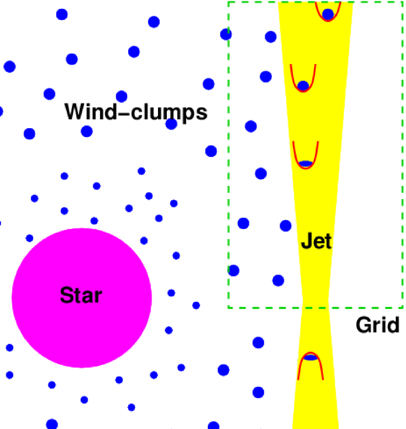
Figure 1: Sketch of the scenario simulated in this work. The green dashed line confines the simulated region.

The inhomogeneities or clumps are modelled as gaussians with $\sigma=R_{\rm c}=3\times 10^{10}$ cm . In reality, the size, mass, and velocity of clumps in stellar winds may follow complex distributions (e.g., Moffat, 2008). However, we have adopted average and representative values for these quantities for simplicity. Bigger and thus less numerous clumps than assumed here would probably have a stronger impact on the jet dynamics, unless they were so few that interactions were rare. The latter may be the case, provided that wind mass seems to concentrate in the small clumps. These small clumps may also be denser than big ones (Moffat, 2008). On the other hand, if $R_{\rm c}\ll 3\times 10^{10}\,{\rm cm}$, then the wind could be effectively considered as homogeneous (as in PBK10). The reason is that clumps cover inside the jet a fraction of its radius: $\chi=R_{\rm c}/R_{\rm j}\sim v_{\rm w}\,R_{\rm c}\,(\pi\,v_{\rm j}\rho_{\rm c}/2L_{\rm j})^{1/2}$ (for a Newtonian jet), where $\rho_{\rm c}=\dot{M}/4\pi fd^{2}v_{\rm w}$ is the clump density. This estimate is based on the clump disruption time, expected to be slightly longer than the clump shock crossing time: $t_{\rm d}\sim R_{\rm c}/c_{\rm c}$, where $c_{\rm c}\sim(2\,L_{\rm j}/\pi v_{\rm j}\rho_{\rm c}R_{\rm j}^{2})^{1/2}$ is the shocked clump sound speed.

Another relevant timescale is the clump acceleration time along the jet, i.e., the time needed to accelerate the clump material up to a speed $\sim c_{\rm c}$, which is $\sim t_{\rm d}$, and because of quick expansion, it takes only several times this value for the clump material to reach $\sim v_{\rm j}$ (see, e.g., Blandford & Koenigl 1979; Klein et al. 1994; ABR09; Pittard et al. 2010; Barkov et al. 2010; for shocked clump evolution in different contexts). For stellar mass-loss rates $\dot{M}\sim 10^{-6}\,M_{\odot}$/yr, $L_{\rm j}\sim 10^{37}$ erg/s, $d\sim 2\times 10^{12}$ cm, and $v_{\rm j}\sim 10^{10}$ cm/s, $\chi$ is $\sim 0.1\,(R_{\rm c}/3\times 10^{10}\,{\rm cm})\,(f/0.1)^{-1/2}$, i.e., clumps with $R_{\rm c}\ll 3\times 10^{10}\,(f/0.1)\,{\rm cm}$ are destroyed in the external jet layers. In this small clump case the wind-jet contact discontinuity should probably develop a turbulent shear-layer faster than in the homogeneous case. Due to destruction, therefore, clumps will not be able to enter the jet if $c_{\rm c}<v_{\rm w}$ within the binary, which occurs at $f>0.1$ for the parameters given above. For relatively weak jets, say $L_{\rm j}\lesssim 10^{36}$ erg/s, these clumps can otherwise cross the whole jet. For $L_{\rm j}\sim 10^{37}$ erg/s, the clumps considered may enter the jet, but it would be difficult for them to escape (see Sect. 5.3).

From the above discussion, we conclude that, under the jet-to-wind momentum flux ratios considered, if the wind is moderately inhomogeneous, say $f\lesssim 0.1$, clumps can effectively penetrate and mass-load the jet, with a penetration effectiveness depending on $R_{\rm c}$. As we show in what follows, clump penetration will have serious consequences on the jet stability and long-term collimation. We note that we have assumed that the properties of the clumps, and the mean separation between them, are constant all over the grid region in which they are located for simplicity. This approximation starts to fail for $z\gtrsim d$, although most of the dynamical impact occurs below or around this distance. It is worthy to mention that for the purpose of this work, the assumed hydrodynamical nature of the jet could be loose to some extent, as long as the magnetic to kinetic pressure ratio in the jet is smaller, say, than $\sim 0.1$. Otherwise, the lateral magnetic pressure can effectively prevent clump penetration into the jet. Moreover, assuming that clumps managed to enter the jet, magnetic pressure could suppress the development of shocks, induce magnetic dissipation and non-thermal activity, and change strongly the clump disruption process, softening or potentiating it (e.g. Jones et al., 1996; Shin et al., 2008). In any case, the flow evolution under a dynamically dominant magnetic field is out of the scope of this work.

3 Simulations

We have performed three numerical simulations using a finite-difference code named Ratpenat, which solves the equations of relativistic hydrodynamics in three dimensions, written in conservation form, using high-resolution-shock-capturing methods. Ratpenat was parallelized with a hybrid scheme with both parallel processes (MPI) and parallel threads (OpenMP) inside each process (see Perucho et al., 2010b). The simulations were performed in Mare Nostrum, at the Barcelona Supercomputing Centre (BSC) with 200 processors, each of them with a duration of 1080 hours, amounting a total of $6.48\times 10^{5}$ computational hours.

3.1 Simulation set-up

The simulations are set-up with an overpressured jet surrounded by the stellar wind of the massive companion. We are thus implicitly assuming that the bow shock generated by the jet when crossing this medium (PBK10) is far enough and the cocoon dilute enough that the wind has occupied the space surrounding the jet itself . The physical size of the grid is, in (base) jet radius units, $160\,R_{\rm j}\,\times\,160\,R_{\rm j}\,\times\,200\,R_{\rm j}$, the last $200\,R_{\rm j}$ in the direction of propagation of the jet ($z$ coordinate). The grid size in the $x$ and $y$ coordinates is divided in two regions, the inner $80\,R_{\rm j}$ around the jet axis having homogeneous resolution, and the outer $40\,R_{\rm j}$ in each direction being formed by cells with increasing size. The resolution in the homogeneous grid is 4 cells/$R_{\rm j}$ at injection, with a total of $320\times 320\times 800$ cells. The extended grid is composed by 80 cells on each side, resulting in a box with $480\times 480\times 800$ cells. In the simulations, $R_{\rm j}=2\times 10^{10}\,\mathrm{cm}$, so the physical size of the grid is $(3.2\times 3.2\times 4)\,\times\,10^{12}$ cm.

In previous works (PB08, PBK10), the wind was simulated as homogeneous, but it was already suggested that a necessary improvement to those simulations should be the inclusion of inhomogeneities. We have done this by randomly adding Gaussian-shaped clumps in the side of the grid from where the stellar wind is injected. The initial number of clumps in the half of the homogeneous grid facing the star, 1500, has been calculated to ensure that the mean wind mass-loss rate is $\approx 10^{-6}\,M_{\odot}$/yr. The clump peak density is 10 times larger than the mean density ($9\times 10^{-15}\mathrm{g/cm^{3}}$), i.e., $9\times 10^{-14}\mathrm{g/cm^{3}}$, and the minimum density between clumps has been fixed to $3\times 10^{-16}\mathrm{g/cm^{3}}$. The whole wind region is set in pressure equilibrium ($P_{\rm w}=1.5\times 10^{-3}\leavevmode\nobreak\ \mathrm{erg/cm^{3}}$) with the higher density regions, and a velocity $v_{\rm w}=2\times 10^{8}\leavevmode\nobreak\ \mathrm{cm/s}$ radial from the star (PB08, PBK10). Figure 2 shows cuts of the initial conditions in pressure and density along the axis of one of the simulated jets, and Fig. 3 shows transversal cuts at $z\simeq 2.2\times 10^{12}\,\mathrm{cm}$.

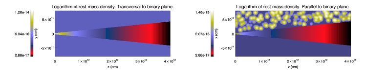
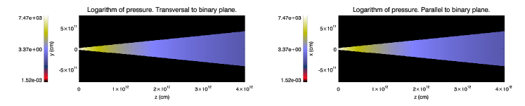
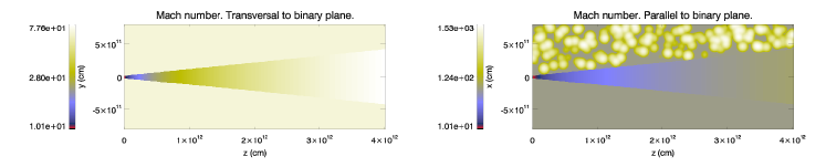
Figure 2: Axial cuts of the jet in the planes perpendicular (left) and parallel (right) to the jet-star plane of rest-mass density (top, $\mathrm{g/cm^{3}}$), pressure (mid, $\mathrm{erg/cm^{3}}$) and Mach number (bottom) for one of the initial models.

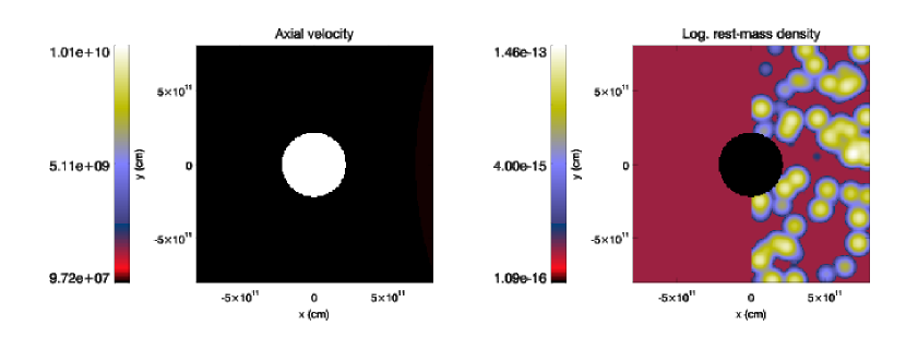
Figure 3: Transversal cuts of the jet at half grid of axial velocity ($\mathrm{cm/s}$) and rest-mass density ($\mathrm{g/cm^{3}}$) for one of the initial models.

We have simulated two jets with different powers, jet A with $L_{\rm j}=3\times 10^{36}\,\mathrm{erg/s}$ and jet B with $L_{\rm j}=10^{37}\,\mathrm{erg/s}$ (to be compared with jet 2 in PBK10). The jets are set-up with a given opening angle but not in pressure equilibrium with the ambient, as this has homogeneous pressure whereas the jet pressure decreases with $z$. The injection point in the grid would be located at $2\times 10^{11}\leavevmode\nobreak\ \mathrm{cm}$ from the compact object, this is, well within the binary system. The jets have both injection densities of $4.2\times 10^{-15}\mathrm{g/cm^{3}}$ and $1.4\times 10^{-14}\mathrm{g/cm^{3}}$, and a velocity $v_{\rm j}=10^{10}\,\mathrm{cm/s}$. Thermal cooling terms, following the approximation used in Myasnikov et al. (1998), have been added to the code to account for the cooling in the clumps. Table 1 summarizes the jet and wind parameters used in the simulations.

We note that to simulate continuous wind injection, the up-wind section of the ambient medium is replenished with clumps when a portion of its volume has been emptied of the original ones. This is done without any effect on the dynamics of the system, as the clumps are added in a region far from the interaction between the jet and the first clumps.

	Density (g/cm3)	Velocity (cm/s)	Mach number	Pressure (erg/cm3)	Power (erg/s)
Jet A (A′)	$4.2\times 10^{-15}$	$10^{10}$	$10$	$2274$	$3\times 10^{36}$
Jet B	$1.4\times 10^{-14}$	$10^{10}$	$10$	$7470$	$10^{37}$
	Min. density (g/cm3)	Max. density(g/cm3)	Mean density (g/cm3)	Pressure (erg/cm3)	Velocity (cm/s)
Wind	$3\times 10^{-16}$	$9\times 10^{-14}$	$9\times 10^{-15}$	$1.5\times 10^{-3}$	$2\times 10^{8}$

Table 1: Jet and wind parameters.

A third simulation was performed to illustrate the evolution of 3 clumps interacting with jet A (jet A^′). The clumps were located at $z=3,\,6$ and $12\times 10^{11}\,\mathrm{cm}$, with increasing distance to the jet in the $x$-direction such that the different clumps start their interaction with the jet subsequently. In Figure 4, the initial distribution of the clumps is shown in the axial density cut of the jet parallel to the star-jet plane.

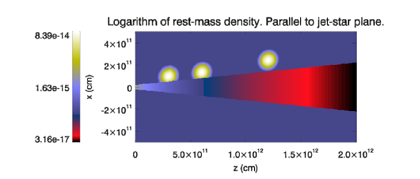
Figure 4: Axial cut parallel to the star-jet plane of rest-mass density ($\mathrm{g/cm^{3}}$) for jet A^′ showing the initial location of the clumps.

4 Results

Jets initially expand due to their overpressure. The expansion is asymmetric, being faster in the direction of propagation of the wind (down-wind). The clumps that enter the jet close to its base are shocked by the expansion of the overpressured jet and eroded by its transversal velocity. The shock generated by this interaction propagates inside the jet, deforming its surface and triggering helical displacements of the jet flow, which add to the deviation of the jet in the direction of the wind further up. The material ablated from the clumps is dragged by the jet, circulates around its surface and generates a turbulent thick shear-layer where is mixed with material of the jet and accelerated in the direction of the latter.

In the central region of the jet, a reconfinement shock is triggered by the irregular ram pressure of the clumpy wind. At this shock, the jet flow is decelerated, favoring clump penetration and clump-jet material mixing downstream. At higher values of coordinate $z$, clumps can fully penetrate into the jet generating bow shocks that cover large fractions of the jet cross section and further decelerate the flow. Thus, the nature of the jet is completely changed within the binary system.

4.1 Jet A

In the case of jet A, the simulation reproduces $\simeq 1700$ s of the jet-wind interaction. Due to the high overpressure of the jet at the injection point, the clumps are destroyed when they get close to the flow at the jet base, although much farther up they can penetrate inside the jet. Figures 5, 6 and 7 show two jet axial cuts, transversal and parallel to the star-jet plane, of rest-mass density, axial velocity and Mach number, respectively. The different images show the temporal evolution, with time increasing downwards. The initial phase of the interaction between the clumps and the jet is seen in the upper panels of each of the figures. The density maps show the generation of an asymmetric reconfinement shock (right panel) due to the ram-pressure of the clumpy wind, and the generation of a rarefied region in the boundaries of the jet produced by the initial expansion into the wind diluted regions. In this slower and more dilute rarefaction region, clumps penetrate easily, deforming the jet surface (see Fig. 6), and the up-wind jet expansion becomes dominated by the interaction with the clumps.

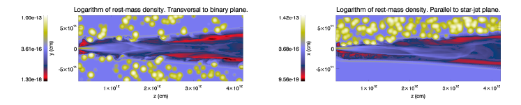
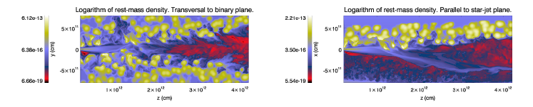
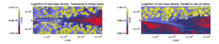
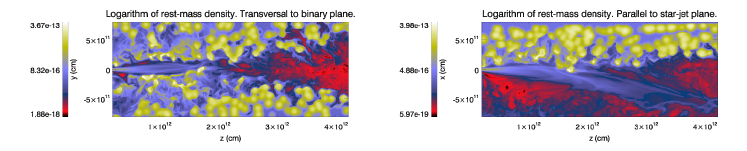
Figure 5: Axial cuts of rest-mass density ($\mathrm{g/cm^{3}}$) at different instants for jet A. Top panels stand for $t=300$ s, second row for $t=1220$ s, $t=1570$ s the third one, and bottom one for the last snapshot of the simulation, at $t=1700$ s.

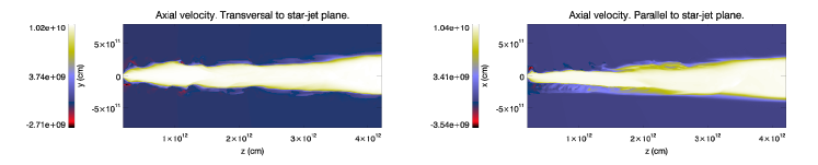
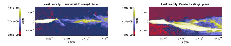
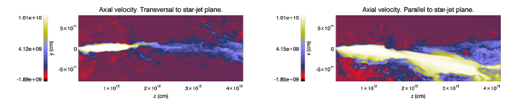
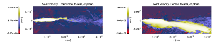
Figure 6: Axial cuts of axial velocity ($\mathrm{cm/s}$) at different instants for jet A. Top panels stand for $t=300$ s, second row for $t=1220$ s, third one for $t=1570$ s, and bottom one for the last snapshot of the simulation, at $t=1700$ s.

At the adopted initial conditions, the jet cools down as it expands along the $z$ axis, accelerating also slightly in the $z$-direction. This implies an increase of the Mach number from the value at injection, $M=10$, to $M\simeq 60$. In the Mach number maps, we can see that, as the time goes by, the maximum Mach numbers in the jet downstream of the reconfinement shock get much smaller than the initial values. Deceleration due to mass entrainement, and heating due to shocks, lead to the formation of transonic and subsonic regions inside the jet flow.

The bottom panels of Figs. 5, 6 and 7 show the last snapshot of the simulation of jet A. The cuts transversal to the star-jet plane (left panels) reveal the jet expansion at small $z$, reconfinement and, once the jet has been deviated, the turbulent region where clump-jet mixing and jet deceleration occur. The cuts parallel to the star-jet plane (right panels) show the effect that a clump entrained just after the reconfinement shock may have, triggering a deviation in the jet direction of more than $10^{\circ}$. As noted above, in the transversal cut to the star-jet plane of rest-mass density (Fig. 5, bottom left panel), it can be seen that the clumps approaching the jet close to the injection point, where the overpressure is large, are destroyed before entering it. In this region, the figures also show complex structures of destroyed clumps mixed with jet material.

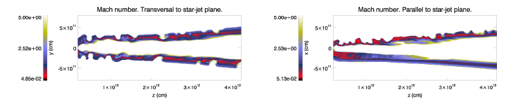
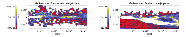
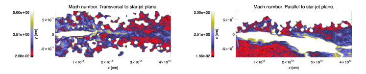
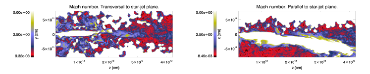
Figure 7: Axial cuts of Mach number at different instants for jet A. Top panels stand for $t=300$ s, second row for $t=1220$ s, third one for $t=1570$ s, and bottom one for the last snapshot of the simulation, at $t=1700$ s. The color scale for this parameter has been saturated at $M=5$, thereby enhancing the contrast inside the jet and thus the location of transonic flows resulting from shocks.

Figure 8 shows cuts of rest-mass density, axial velocity and Mach number transversal to the jet axis for jet A at the injection point, $\sim 1/4,\,1/2$, and $3/4$ of the grid length ($z=2\times 10^{11},\,1.2,\,2.2,$ and $3.2\times 10^{12}\,\mathrm{cm}$). The first cut shows the disruption of the clumps as soon as they get close to the jet, whereas the jet Mach number and velocity keep their initial values. At one quarter of the grid ($z\simeq 1.2\times 10^{12}\,\mathrm{cm}$), the jet presents an elongated structure in the down-wind direction. In the up-wind direction, rarefied jet material left after the initial jet expansion forms filaments between the clumps. At this point, some regions of the jet section keep a large fraction of the original Mach number and axial velocity, but some others already show signs of the action of the reconfinement shock. At $z\simeq 2.2\times 10^{12}\,\mathrm{cm}$, the jet flow has already gone through this shock, and the wind thrust has managed to deviate its original direction. Although the flow has reexpanded and partially recovered the strongly supersonic nature, the impact of the reconfinement shock has caused a noticeable decrease in velocity from the original values. At $z\simeq 3.2\times 10^{12}\,\mathrm{cm}$ the jet shows a large radial displacement and irregular morphology. Overall, the jet section is clearly displaced from the center of the grid. Although the jet keeps a high axial velocity at this position, the density cuts show an increase of more than one order of magnitude with respect to the original value ($\simeq 3.2\times 10^{-17}\,\mathrm{g/cm^{-3}}$) in some regions of the jet at this position.

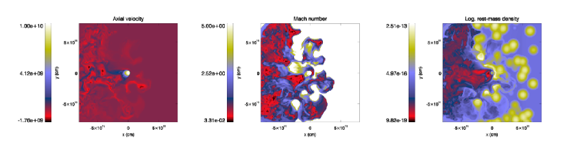
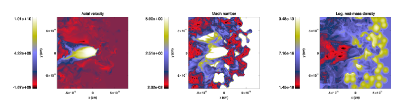
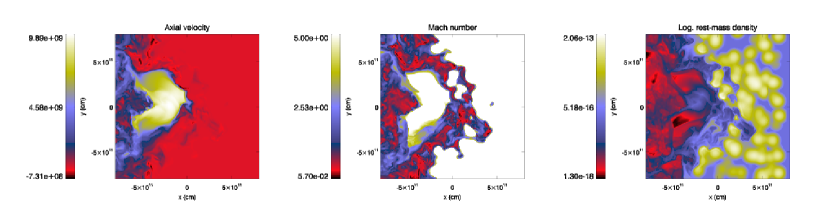
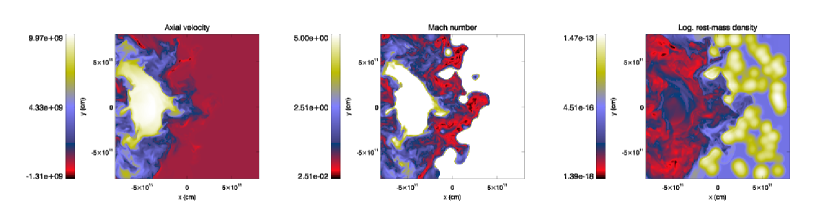
Figure 8: Transversal cuts of rest-mass density ($\mathrm{g/cm^{3}}$), axial velocity ($\mathrm{cm/s}$) and Mach number for the last snapshot ($t=1700$ s) of jet A, at $z=2\times 10^{11},\,1.2,\,2.2,$ and $3.2\times 10^{12}\,\mathrm{cm}$. The color scale of the Mach number has been saturated at $M=5$.

4.2 Jet B

This simulation reproduces the jet-wind interaction during $t\simeq 2000$ seconds for jet B, with $L_{\rm j}=10^{37}$ erg/s. The same qualitative explanation for the evolution of jet A applies also to jet B. However, the overpressure of the jet is larger, and the reconfinement shock, produced by the global clumpy wind impact, appears further downstream than in jet A. There are interesting differences with respect to jet A due to the entrainement of a clump in jet B at $z\simeq 2.2\times 10^{12}\,\mathrm{cm}$, which is favored by the strong decrease of the inertia of the jet downstream of the reconfinement shock. This clump generates a strong bow shock that eventually covers the whole jet section. Behind the bow shock the jet is decelerated and a turbulent layer is formed. Once the clump is destroyed, the jet may recover its previous configuration, but the constant injection of further inhomogeneities in the wind makes it unlikely. This event is very illustrative of the clumpy wind disruptive effects. Figures 9, 10 and 11 show the evolution of jet B with time through panels of rest-mass density, axial velocity and Mach number, respectively. The large overpressure of the jet allows some filaments of jet material to propagate between clumps in the up-wind direction. Again, the jet becomes subsonic downstream of the region where the reconfinement shock and the bow shocks generated by the clumps occur ($z\simeq 2.4\times 10^{12}\,\mathrm{cm}$).

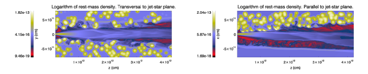
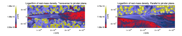
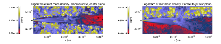
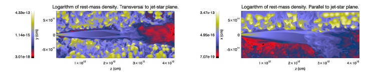
Figure 9: Axial cuts of rest-mass density ($\mathrm{g/cm^{3}}$) at different instants for jet B. Top panels stand for $t=470$ s, second row for $t=1640$ s, third one for $t=1770$ s and bottom one for the last snapshot of the simulation, at $t=1970$ s.

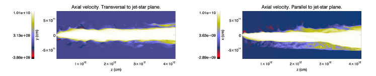
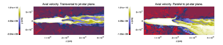
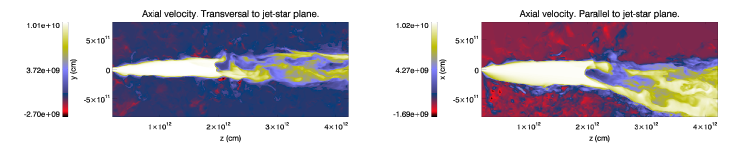
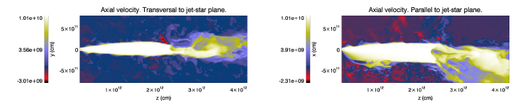
Figure 10: Axial cuts of axial velocity ($\mathrm{cm/s}$) at different instants for jet B. Top panels stand for $t=470$ s, second row for $t=1640$ s, third one for $t=1770$ s and bottom one for the last snapshot of the simulation, at $t=1970$ s.

Figure 12 shows transversal cuts of axial velocity, Mach number and rest-mass density at the last snapshot of the simulation at the jet injection position, $z\simeq 2\times 10^{11}\,\mathrm{cm}$, and at $z=1.2,\,2.2,$ and $3.2\times 10^{12}\,\mathrm{cm}$. At the injection point, the image obtained is very similar to that from jet A (see upper panels in Fig. 8). At $z=1.2\times 10^{12}\,\mathrm{cm}$ and $2.2\times 10^{12}\,\mathrm{cm}$, the jet is still well collimated with large velocity and Mach number. In these cuts, filaments of material travelling in the up-wind direction can be observed. The last set of images (bottom row), at $z=3.2\times 10^{12}\,\mathrm{cm}$, shows the effect of the entrained clumps. In the left panel, the traces of the clumps can be seen as low velocity regions, resulting also in transonic or even subsonic velocities as indicated by the Mach number maps. The initial density of the jet at this point was $\rho\simeq 5\times 10^{-17}\,\mathrm{g/cm^{-3}}$ at the start of the simulation, whereas the right panel shows densities one order of magnitude larger within the jet, indicating efficient assimilation of wind material.

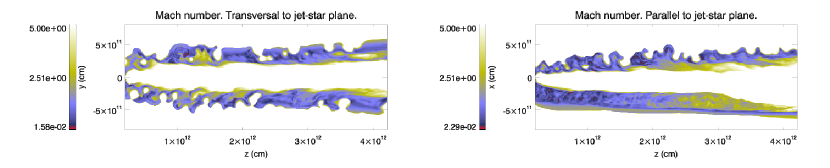
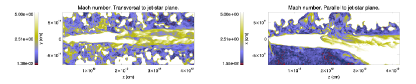
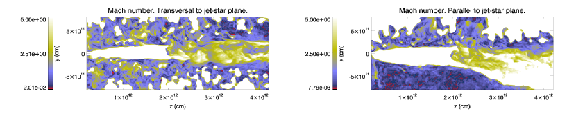
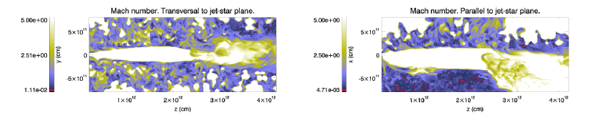
Figure 11: Axial cuts of Mach number at different instants for jet B. Top panels stand for $t=470$ s, second row for $t=1640$ s, third one for $t=1770$ s and bottom one for the last snapshot of the simulation, at $t=1970$ s. As in Fig. 7, the color scale is saturated at $M=5$.

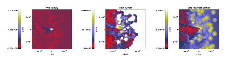
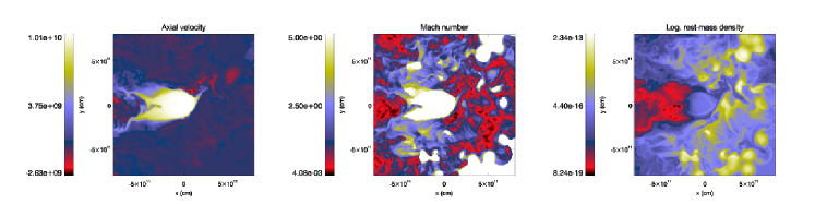
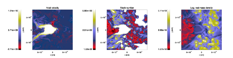
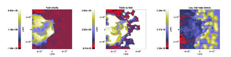
Figure 12: Transversal cuts of rest-mass density ($\mathrm{g/cm^{3}}$), axial velocity ($\mathrm{cm/s}$) and Mach number for the last snapshot ($t=1900$ s) for jet B, at $z=0.2,\,1.2,\,2.2,$ and $3.2\times 10^{12}\,\mathrm{cm}$. The color scale of the Mach number has been saturated at $M=5$.

4.3 Jet A^′

The previous simulations show very complex structures and dynamics. In order to have a clearer idea of the processes taking place, we repeated the simulation of jet A with only three clumps located initially at $z=0.3,\,0.6$ and $1.2\times 10^{12}\,\mathrm{cm}$, as shown in Fig. 4. The simulation was stopped after $t\simeq 1000$ seconds. Figures 13 and 14 show the time evolution of the interaction of the clumps with the jet. The first clump is destroyed in the jet surface, with little dynamical impact on the jet. Otherwise, the second clump triggers a shock that propagates inside the jet, although the clump itself is also destroyed before entering into the jet. Between the first two clumps, jet material shocked by the second clump rises due to the local pressure gradients in the up-wind direction. The third clump shows the same behavior as observed in the simulation of jet B, being able to enter into the jet before being destroyed, and generating a strong bow shock that causes jet expansion, deceleration and significant mass-load.

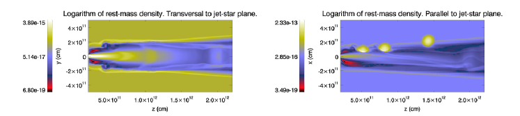
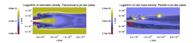
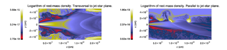
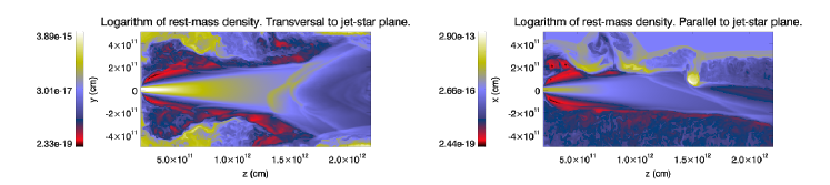
Figure 13: Axial cuts of rest-mass density ($\mathrm{g/cm^{3}}$) at different instants for jet A’. Top panels stand for $t=170$ s, second row for $t=320$ s, third one for $t=780$ s, and bottom one for the last snapshot of the simulation, at $t=970$ s.

Figure 15 shows transversal cuts of axial velocity, Mach number and density (as in Figs. 8 and 12). In this case, the cuts are done at $z\simeq 0.25,\,0.75,\,1,\,1.5$ and $1.75\times 10^{12}\leavevmode\nobreak\ \mathrm{cm}$. The structures are much clearer in these plots due to the small number of clumps. At $z=0.75\times 10^{12}\leavevmode\nobreak\ \mathrm{cm}$ we see the disrupted rests of the first clump (originally at $z=0.3\times 10^{12}\leavevmode\nobreak\ \mathrm{cm}$, see bottom panel of Fig. 13). Initially, this clump crossed the shock driven by the jet in the diluted medium, and was disrupted at the jet surface. This interaction already implies some loss of initial jet thrust, which is transferred to the clump remains that become part of the jet flow. The shock that this interaction generates is observed as a bow-like structure inside the jet inner boundary in the Mach number and density panels at higher values of coordinate $z$. The next set of cuts, at $10^{12}\,\mathrm{cm}$, shows a snapshot of the disruption of the second clump. This process is here at an earlier stage than that of the first clump. At $z=1.5$ and $1.75\times 10^{12}\,\mathrm{cm}$, one can see the clear effect of the clump located at $1.4\times 10^{12}\,\mathrm{cm}$, which generates a bow-like structure entering the jet and a cometary tail, crossed by the transversal cuts, of jet dragged material (see bottom panels in Figs. 13 and 14). The other bow-like waves, visible mainly at $x<0$ in the images, are the bow shocks generated by the interaction with the clumps upstream of this position. At $z=1.75\times 10^{12}\,\mathrm{cm}$, the jet is dominated by the bow-like structures triggered by the interactions upstream, and the cometary-like tail from the third clump is seen at $x>0$ region. The faster regions of the jet are those that have not been crossed by any of these shocks, i.e., those that lie at the smaller values of $x$. The jet keeps a large velocity in those particular regions, but it is in general efficiently mass-loaded and decelerated.

Overall, the picture is similar to that shown in simulations of jets A and B, showing that only a few clumps generated by inhomogeneities in the injection of the wind could produce already significant changes in the properties of the jet flow.

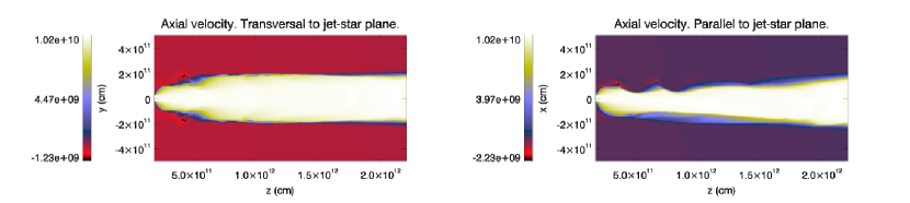
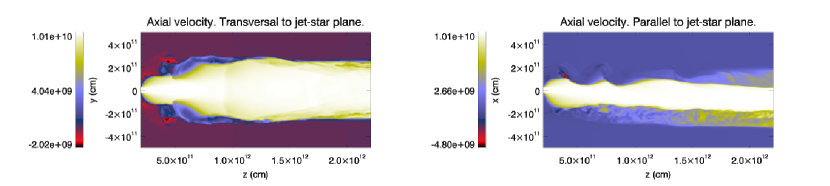
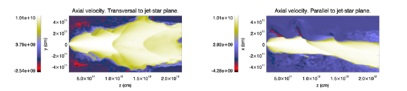
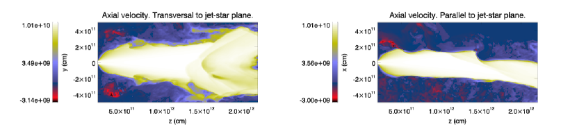
Figure 14: Axial cuts of axial velocity ($\mathrm{cm/s}$) at different instants for jet A’. Top panels stand for $t=170$ s, second row for $t=320$ s, third one for $t=780$ s, and bottom one for the last snapshot of the simulation, at $t=970$ s.

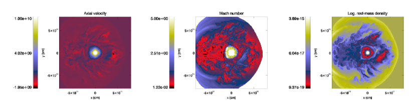
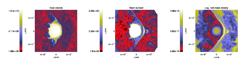
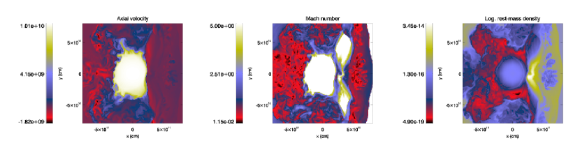
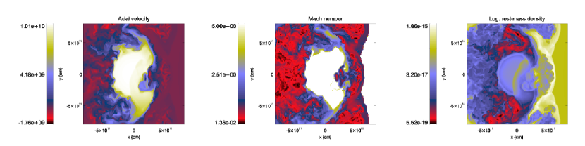
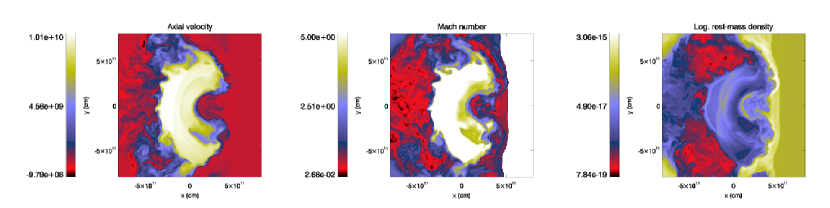
Figure 15: Transversal cuts of rest-mass density ($\mathrm{g/cm^{3}}$), axial velocity ($\mathrm{cm/s}$) and Mach number for the last snapshot ($t=970$ s) of jet A’ at $z\simeq 0.25,\,0.75,\,1,\,1.5$ and $1.75\times 10^{12}\leavevmode\nobreak\ \mathrm{cm}$. The color scale of the Mach number has been saturated at $M=5$.

5 Discussion

5.1 Jet propagation

The simulated jets are strongly deviated from their original direction and show disrupted morphologies at the end of the calculations. Initially, the first interactions at small values of $z$ trigger helical patterns that, in the absence of further perturbations, could couple to Kelvin-Helmholtz unstable modes. However, the reconfinement shock triggered by the ram pressure of the clumpy wind on the jet plus individual interactions with multiple clouds downstream of this shock, generate non-linear structures that are most important for the jet evolution. The position of the reconfinement shock is located within the binary region, as predicted by PB08. There, the jet is decelerated and heated, thus becoming even weaker relative to the wind thrust, as also shown in PB08 and PBK10. In the present case, the clumps from the up-wind region can penetrate in the jet already at $z\sim 1-2\times 10^{12}$ cm, generating additional bow-like shocks and decelerating even more the jet flow. The deviation of the jet favors the presence of a region, on the down-wind side of the jet, to which, by the end of simulations, the clump bow shocks and jet mixing have still not reached. In this region, the flow keeps a relatively large axial velocity in this direction. However, both shocks and clump-mixed jet material should eventually fill the whole jet at larger $z$, so the description just presented (see Figs 9, 10 and 11) can be extended to the whole jet cross section. As a result, farther downstream the jet becomes mass-loaded, slow and transonic. Although a similar result was already obtained in the homogeneous wind case (PB08, PBK10), wind clumping significantly potentiates jet destruction.

When comparing jet B in this work with jet 2 in PBK10, it is remarkable that the presence of a forward shock and the absence of clumps in the latter have a strong influence on the long-term evolution of the jet. The jet-driven forward shock in the wind and the corresponding cocoon (see PBK10) keep the wind at some distance from the jet. If a homogeneous wind were already in contact with jet 2 in PBK10, a smooth shear layer would form. Otherwise, the presence of clumps in jet B enhances the thrust locally in the wind, increasing mass, momentum and energy exchange. Jet 2 in PBK10 thus shows a larger degree of collimation and is just slightly deviated from its original direction of propagation, contrary to what we observe in the case of jet B in this paper. From this work we can conclude that jet luminosities $L_{\rm j}\gtrsim 10^{37}\,\dot{M}_{-6}\mathrm{erg/s}$ ($\dot{M}_{-6}=\dot{M}/10^{-6}\,M_{\odot}$/yr) are needed if the jet is not to be destroyed when crossing the binary system. We notice that these dynamical arguments favor $L_{\rm j}\gtrsim 10^{37}$ and $10^{38}$ erg/s in the HMMQ Cygnus X-1 and Cygnus X-3, respectively. The cocoon/clumpy wind case deserves few words. This situation takes place when the forward shock is well within the binary system, and the cocoon pressure is high, preventing clumps from entering the cocoon. When the forward shock has reached the outskirts of the binary, the cocoon pressure drops quickly (PBK10), allowing wind clumps to penetrate into the cocoon and reach the jet, and eventually dissipate the cocoon away.

5.2 Clump evolution

In jets A and B, those clumps reaching the jet relatively close to its base are destroyed just by jet expansion or erosion. These interactions trigger a shock wave that propagates inside the jet, and when interactions are frequent such a wave forces the strongly disruptive asymmetric recollimation shock. This phenomenon is illustrated in Fig. 13), in which the first clump is completely destroyed by jet expansion, whereas the second one, even when it does not fully penetrate into the jet, triggers a shock strong that propagates all through the latter lasting for the whole simulation (several $t_{\rm d}$; see Sect. 2). The clump at the highest $z$ in jet A’ ($1.4\times 10^{12}$ cm) is shocked but still not significantly disrupted by instabilities after few $t_{\rm d}$. Later, this clump could be destroyed or may eventually escape the jet, although jet bending in the down-wind direction makes the latter unlikely. When clumps are disrupted inside the jet, all the clump mass is entrained by the flow. The level of mass loading can be easily estimated from the amount of clumps entering into the jet per time unit: $\dot{N}_{\rm cj}\sim(\eta/4\pi)(3\dot{M}/4\pi R_{\rm c}^{3}\rho_{\rm c})\approx 0.02$ clump/s or $\approx 5\times 10^{17}$ g/s. This is $\sim 3$ times more mass flux than in the jet. Therefore, jet deceleration due to mass loading can be very efficient, as is most clearly seen in the simulation results for jet B. The implications also apply to faster and lighter, but equally powerful jets. Even if a strongly relativistic flow is injected at the jet base, for similar jet (relativistic) ram pressures clump penetration into, and mixing with, the jet will also occur. This will mass-load and brake the jet very quickly.

The qualitative dynamical scenario presented in ABR09 is validated by our numerical work in a semi-quantitative way. Remarkably, as hinted in ABR09, the clump interaction with many clumps will reduce the jet kinetic luminosity and also its ram pressure. In this way, clumps can actually keep their integrity longer, and penetrate farther inside the jet, even for moderate $f$-values.

5.3 Radiation considerations

In ABR09, the radiation produced by a clump inside a HMMQ jet was calculated. Given the compactness of the considered region, i.e. the bow shock formed around the clump, radio emission was negligible. The luminosities of synchrotron X-ray, and (stellar photon) IC gamma-rays, dominated the non-thermal output, with their values anticorrelating depending on the magnetic field. Based on that work, and extending the study to the multi-clump/jet interaction case simulated here, we qualitatively discuss in what follows the expected emission.

The typical number of clumps inside the jet, at the binary scales, can be estimated as $N_{\rm cj}\sim$ few times $t_{\rm d}\,N_{\rm cj}$, i.e. $\gtrsim 10$ for the wind and jet properties adopted in this work (recall that the real clump lifetime is longer than $t_{\rm d}$). Since $t_{\rm d}\sim 100\,{\rm s}<R_{\rm j}/v_{\rm w}\sim 1000$ s, clump destruction will likely limit $N_{\rm j}$ instead of jet-crossing escape. Although the jet can be quite disrupted and mass-loaded at the borders of the system, one can derive an estimate for the non-thermal emission, which depending on $B^{2}/8\pi u_{*}$ ($u_{*}=L_{*}/4\pi d^{2}c$) will be released either through synchrotron (keV-MeV) or IC (GeV-TeV). We note that, for $B$-values well below equipartition with the non-thermal electron energy density, synchrotron self-Compton may also contribute to the IC component, although we neglect this component here for analysis simplicity. We also do not consider non-radiative losses or hadronic processes, but refer to ABR09.

Assuming a 10% efficiency for the kinetic-to-non-thermal energy transfer in clump bow shocks, and accounting for the clump-jet covering fraction $\xi_{\rm cj}\sim(R_{\rm c}/\eta d)^{2}$, the high-energy emission can reach luminosities of $\sim 0.1\,N_{\rm cj}\,\xi_{\rm cj}\,L_{\rm j}\sim 0.01\,L_{\rm j}$. This value may lead to a source that may be detectable in GeV ($B^{2}/4\pi u_{*}<1$) and even in TeV ($B^{2}/4\pi u_{*}\ll 1$), showing persistent plus fluctuating variability components (Owocki et al., 2009). Strong TeV photon absorption may be avoided since most of the emission would come from the borders of the binary (e.g., Bosch-Ramon & Khangulyan, 2009). For $B^{2}/4\pi u_{*}\gtrsim 1$, synchrotron soft gamma-rays would dominate the non-thermal output. Thermal radiation, peaking at several keV, from the shocked clumps may be also present (ABR09). but it is minor for the adopted clump properties.

It is noteworthy that for a steep clump-size distribution (see Sect. 2), i.e. with most of the clump-jet interaction occurring in a quasi-homogeneous wind regime, still several big clumps could enter the jet. This would likely lead to a lower level of persistent emission, but time to time chance would bring few big and dense clumps together inside the jet, rendering sudden and bright events with durations of a few $1000\,(R_{\rm c}/10^{11}\,{\rm cm})\,(c_{\rm c}/10^{8}\,{\rm cm})^{-1}$ s (ABR09). These statistically expected violent events could be related to a temporary complete destruction of the jet for large enough clumps.

Although the jets of microquasars present a complex phenomenology of their own (Fender et al., 2004, 2009), on top of that it is expected additional phenomena linked to the jet-wind interaction in HMMQ, as this and previous works (PB08, PBK10) show. Since the jet power is strongly linked to the mass-loss rate, HMMQ jets detectable in X-rays or gamma-rays will be probably found in systems with moderate-to-strong winds. Therefore, unless particle acceleration is negligible in clump bow shocks, HMMQ phenomenology at high-energies must be strongly affected by them, showing wind-related strong variability at high energies unless the wind is quite homogeneous or clumps with $R_{\rm c}>10^{10}$ cm are completely missing. Concerning (powerful) transient ejections, usually associated to X-ray state transitions, we note that such an ejections will require some time to form. If this takes hours, the wind will have time to surround the transient jet. Then, the clump impact will be as described here unless the jet is too powerful. If powerful blobs would appear as discrete even at the scales of the binary, they may have too much inertia to be significantly affected by the wind.

The dynamical impact of the stellar wind on the jet, enhanced by clumpiness, should not be neglected when interpreting radio emission from HMMQ. Even if jets escape from disruption, the enhanced jet entropy and bending, even by small angles ($\sim 10^{\circ}$), could have observational consequences. The reason is that bending pushes jet material farther from the orbital plane axis, increasing the strength of the Coriolis force exerted by the stellar wind and the orbital motion. The farther away from this axis the jet reaches, the stronger this force gets, enhancing jet heating, turbulence and bending. Although quantitative predictions call for a detailed study, this region may be observationally probed using VLBI techniques. Far enough from the binary, once the jet has become too wide to be affected by the orbital motion, a collimated supersonic flow may form again. If the energy and momentum fluxes kept enough anisotropy after crossing the system and suffer from orbital motion, given a negligible external pressure a jet-like structure could form again and propagate unstopped up to pc scales, terminating in the ISM (e.g. Bordas et al., 2009; Bosch-Ramon et al., 2011; Yoon et al., 2011). Despite the different outflow geometry, similar phenomena are also expected in high-mass binaries hosting non-accreting pulsars (see Bosch-Ramon & Barkov, 2011).