Generic singular configurations of linkages

Abstract.

We study the topological and differentiable singularities of the configuration space  ${\mathcal{C}}(\Gamma)$   of a mechanical linkage $\Gamma$ in  ${\mathbb{R}}^{d}$,  defining an inductive sufficient condition to determine when a configuration is singular. We show that this condition holds for generic singularities, provide a mechanical interpretation, and give an example of a type of mechanism for which this criterion identifies all singularities.

0. Introduction

The mathematical theory of robotics is based on the notion of a mechanism consisting of links, joints, and rigid platforms. The mechanism type is a simplicial (or polyhedral) complex  ${\mathcal{T}}_{\Gamma}$,  where the parts of dimension $\geq 2$  correspond to the platforms, and the complementary one-dimensional graph corresponds to the links (=edges) and joints (=vertices). The linkage (or mechanism) $\Gamma$ itself is determined by assigning fixed lengths to each of the links of  ${\mathcal{T}}_{\Gamma}$.  See [Me, Se, T] and [F] for surveys of the mechanical and topological aspects, respectively.

0.1.

Configuration spaces. Here we concentrate on the most prevalent type of mechanism  ${\mathcal{T}}_{\Gamma}$:  namely, a finite $1$-dimensional simplicial complex (undirected graph), with $N$ vertices and $k$ edges. Note that a rigid platform is completely specified by listing the lengths of all its diagonals (i.e., the distance between any two vertices), so we need not list the platforms explicitly. Our results actually hold also for the case when some links of $\Gamma$ are prismatic (or telescopic)  –  i.e., have variable length  –  but for simplicity we deal here with the fixed-length case only.

A length-preserving embedding of the vertices of the linkage $\Gamma$ in a fixed ambient Euclidean space  ${\mathbb{R}}^{d}$   is called a configuration of $\Gamma$. In applications, $d$ is most commonly $2$ or $3$. The set of all such embeddings, with the natural topology (and differentiable structure), is called the configuration space of $\Gamma$, denoted by  ${\mathcal{C}}(\Gamma)$.  Such configuration spaces have been studied intensively, with the hope of extracting useful mechanical information from their topological or geometric properties. Much of the mathematical literature has been devoted to the special case when $\Gamma$ is a closed chain (polygon): see, e.g., [FTY, Hau, HK, KM1, KM2, MT]. However, the general case has also been treated (cf. [Ho, Ka, KTs, KM3, OH, SSB1, SSB2]).

0.2.

Singularities. There are two main types of singularities which arise in robotics. The kinematic singularities of a mechanism, which appear as singularities of work and actuation maps defined on  ${\mathcal{C}}(\Gamma)$   (§1.5), have obvious mechanical interpretations, and have been studied intensively (see, e.g., [GA], [Me, §6.2], and [ZFB]). On the other hand, the topological or differentiable singularities of the configuration space  ${\mathcal{C}}(\Gamma)$   itself have not received much attention in the literature since [Hu], aside from some special examples (see, e.g., [F, KM2] and [ZBG]).

For any linkage $\Gamma$, the configuration space  ${\mathcal{C}}(\Gamma)$   is the zero set of a smooth function  $\lambda:{\mathbb{R}}^{Nd}\to{\mathbb{R}}^{k}$   (see §1.1 below), so that  ${\mathcal{C}}(\Gamma)$   is typically a smooth manifold (when  $\vec{\mathbf{0}}\in{\mathbb{R}}^{d}$   is a regular value of $\lambda$), and even if not, “most” points of  ${\mathcal{C}}(\Gamma)$   are smooth, since a simple necessary condition for a point ${\mathcal{V}}$ in  ${\mathcal{C}}(\Gamma)$   to be singular is that  $\operatorname{Rank}(\operatorname{d}\!\lambda_{{\mathcal{V}}})<k$.  Thus we are in the common situation where it is relatively straightforward to identify configurations which are possibly singular, but not so easy to pinpoint when this is in fact so.

Our goal in this paper is threefold:

1. To provide a straightforward inductive description of a sufficient condition for a configuration ${\mathcal{V}}$ to be differentiably singular (in fact, this will imply that ${\mathcal{V}}$ is even a topological singularity)  –  see Proposition 3.8 and Theorem 4.9.

2. To show that this condition applies generically (that is, to all but a positive-codimension subset of the singular locus $\Sigma$)  –  see Remarks 3.7 and 4.8.

3. To obtain a mechanical interpretation for all singularities in the configuration space of a linkage $\Gamma$ as a tangential conjunction of two kinematic singularities of type I (cf. [GA]) for complementary sub-mechanisms of $\Gamma$  –  see Remark 4.10.

The third goal is completely achieved only in the plane (for  $d=2$),  since the model we use for configuration spaces is not completely realistic for rigid rods in  ${\mathbb{R}}^{3}$.  See Remark 1.7 below for an explanation of the difficulties involved.

0.3 Remark.

Since the function  $f:{\mathbb{R}}^{Nd}\to{\mathbb{R}}^{k}$   defining the configuration space is a quadratic polynomial (cf. §1.1),  ${\mathcal{C}}(\Gamma)$   is actually a real algebraic variety. Thus any topological or differentiable singularity ${\mathcal{V}}$ is in particular an algebraic singularity (cf. [Sh, Ch. II, §1.4]). Somewhat more surprisingly, every real algebraic variety is a union of components of the configuration space of some planar linkage  ($d=2$)    –  see [KM3, Ki, JS]. Thus our results here appear to be statements about any real algebraic variety.

However, the point we wish to make here is not that the cone singularities are the most common ones in algebraic varieties; it is rather the mechanical interpretation of the generic singularities, and the mechanical underpinnings of the inductive process described in Section 4.

In fact, while the topological, differentiable, and geometric structures on configuration spaces of linkages can be used to study their mechanics (cf. [KM2, KTe]), the algebraic structure usually plays no role (but see [C]).

0.4.

Organization. In Section 1 we briefly review some of the basic notions used in this paper. In Section 2, various concepts of local equivalences of configuration spaces are defined; these help to simplify the study of singular points. In Section 3 we explain the role played by pullbacks of configuration spaces. This is applied in Section 4 to provide an inductive construction, which is used both to describe the sufficient condition mentioned in §0.2(b), and to show that they are indeed singular points. An example is studied in detail in Section 5.

0.5 Acknowledgements.

We wish to thank the referee for his or her comments.

1. Background on configuration spaces

We first recall some general background material on the construction and basic properties of configuration spaces. This also serves to fix notation, which is not always consistent in the literature.

1.1 Definition.

Consider an abstract graph  ${\mathcal{T}}_{\Gamma}$   with vertices $V$ and edges  $E\subseteq V^{2}$.  A linkage (or mechanism) $\Gamma$ of type  ${\mathcal{T}}_{\Gamma}$   is determined by a function  $\ell:E\to{\mathbb{R}}_{+}$   specifying the length  $\ell_{i}$   of each edge  $e_{i}$   in  $E=\{e_{i}=(u_{i},v_{i})\}_{i=1}^{k}$   (subject to the triangle inequality as needed). We write  $\vec{\ell}^{2}:=(\ell_{1}^{2},\dotsc,\ell_{k}^{2})\in{\mathbb{R}}^{E}$   for the vector of squared lengths.

The set of all embeddings of $V$ in an ambient Euclidean space  ${\mathbb{R}}^{d}$   is an open metric subspace of  $({\mathbb{R}}^{d})^{V}$,  denoted by  $\operatorname{Emb}^{d}({{\mathcal{T}}_{\Gamma}})$.  We have a squared length map  $\lambda:\operatorname{Emb}^{d}({{\mathcal{T}}_{\Gamma}})\to{\mathbb{R}}^{E}$   with  $\lambda(u_{i},v_{i}):=\|\varphi(u_{i})-\varphi(v_{i})\|^{2}$,  and the configuration space of the linkage  $\Gamma=({\mathcal{T}}_{\Gamma},\ell)$   is the metric subspace  ${\mathcal{C}}(\Gamma):=\lambda^{-1}(\vec{\ell}^{2})$   of  $\operatorname{Emb}^{d}({{\mathcal{T}}_{\Gamma}})$.  A point  ${\mathcal{V}}\in{\mathcal{C}}(\Gamma)$   is called a configuration of $\Gamma$. Note that $\lambda$ is an algebraic function of  ${\mathcal{V}}\in{\mathbb{R}}^{dN}$   (which is why the lengths were squared), so  ${\mathcal{C}}(\Gamma)$   is a real algebraic variety.

1.2 Remark.

By [Hi, I, Theorem 3.2], we know that  ${\mathcal{C}}(\Gamma)$   is a smooth manifold if  $\vec{\ell}^{2}$   is a regular value of $\lambda$: that is, if its differential  $\operatorname{d}\!\lambda_{{\mathcal{V}}}$   is of maximal rank for every  ${\mathcal{V}}\in\operatorname{Emb}^{d}({{\mathcal{T}}_{\Gamma}})$   with  $\lambda({\mathcal{V}})=\vec{\ell}^{2}$.

However, for some mechanism types  ${\mathcal{T}}_{\Gamma}$,  this condition may not be generic: there exist mechanism types  ${\mathcal{T}}_{\Gamma}$   and an open set $U$ in  ${\mathbb{R}}^{dN}$   consisting of non-regular values of  $F^{\Gamma}$.  This means that for each  $\vec{\ell}^{2}_{0}\in U$,  the configuration space  ${\mathcal{C}}(\Gamma_{\vec{\ell}^{2}_{0}}):=\lambda^{-1}(\vec{\ell}^{2}_{0})$   has at least one configuration  ${\mathcal{V}}\in{\mathcal{C}}(\Gamma_{\vec{\ell}^{2}_{0}})$   such that $\lambda$ not a submersion at ${\mathcal{V}}$. See [SSB2] for an example.

1.3.

Isometries of configuration spaces. The group  $\operatorname{Euc}^{d}$   of isometries of the Euclidean space  ${\mathbb{R}}^{d}$   acts on the space  ${\mathcal{C}}(\Gamma)$.  When $\Gamma$ has a rigid “base platform” $P$ of dimension $\geq d-1$,  this action is free. In this case we can work with the “restricted configuration space”  ${\mathcal{C}}(\Gamma)/\operatorname{Euc}^{d}$,  and the quotient map has a continuous section (equivalent to choosing a fixed location in  ${\mathbb{R}}^{d}$   for $P$). See §5.1 for an example of such a $\Gamma$.

In general, certain configurations (e.g., those contained in a proper linear subspace $W$ of  ${\mathbb{R}}^{d}$)  may be fixed by certain transformations (those fixing $W$), so the action of  $\operatorname{Euc}^{d}$   is not free.

1.4 Definition.

Choose a fixed vertex  $\mathbf{x}_{\star}$   of $\Gamma$ as its base-point: the action of the translation subgroup  $T\cong{\mathbb{R}}^{d}$   of  $\operatorname{Euc}^{d}$   on  $\mathbf{x}_{\star}$   is free, so its action on  ${\mathcal{C}}(\Gamma)$   is free, too, and we call the quotient space  ${\mathcal{C}}_{\ast}(\Gamma):={\mathcal{C}}(\Gamma)/T$   the pointed configuration space for $\Gamma$. Thus  ${\mathcal{C}}(\Gamma)\cong{\mathcal{C}}_{\ast}(\Gamma)\times{\mathbb{R}}^{d}$,  and a pointed configuration (i.e., an element of  ${\mathcal{C}}_{\ast}(\Gamma)$)  is simply an ordinary configuration expressed in terms of a coordinate frame for  ${\mathbb{R}}^{d}$   with the origin at  $\mathbf{x}_{\star}$.

If we also choose a fixed link $\vec{\mathbf{v}}$ in $\Gamma$ starting at  $\mathbf{x}_{\star}$,  we obtain a smooth map  $p:{\mathcal{C}}_{\ast}(\Gamma)\to S^{d-1}$   which assigns to a configuration ${\mathcal{V}}$ the direction of $\vec{\mathbf{v}}$. The fiber  $\widehat{{\mathcal{C}}}_{\ast}(\Gamma)$   of $p$ at  $\vec{\mathbf{e}}_{1}\in S^{d-1}$   will be called the reduced configuration space of $\Gamma$. Note that the bundle  ${\mathcal{C}}_{\ast}(\Gamma)\to S^{d-1}$   is locally trivial.

1.5 Definition.

A mechanism $\Gamma$ may be equipped with a special point  $\mathbf{x}_{e}$    –  in engineering terms this is the “end-effector” of $\Gamma$, whose manipulation is the goal of the mechanism. We think of  $\Delta:=\{\mathbf{x}_{e}\}$   as a sub-mechanism of $\Gamma$ (more generally, we could choose any rigid sub-mechanism). Assuming that the base-point  $\mathbf{x}_{\star}$   of $\Gamma$ is not  $\mathbf{x}_{e}$,  the inclusion  $j:\Delta\hookrightarrow\Gamma$   induces a map of configuration spaces  $j^{\ast}:{\mathcal{C}}_{\ast}(\Gamma)\to{\mathcal{C}}(\Delta)$,  whose image ${\mathcal{W}}$ is called the work space of the mechanism. The work map  $\psi:{\mathcal{C}}_{\ast}(\Gamma)\to{\mathcal{W}}$   of $\Gamma$ is the factorization of  $j^{\ast}$   through ${\mathcal{W}}$ (which is not always a smooth manifold).

1.6 Example.

Now consider a closed $5$-chain  $\Gamma_{\operatorname{cl}}^{5}$,  as in Figure 1, with end-effector  $\mathbf{x}_{e}=\mathbf{x}^{({2})}$.  Here the direction of  $\vec{\mathbf{v}}:=\mathbf{x}^{({4})}-\mathbf{x}^{({0})}$   is fixed.

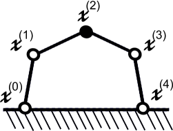
Figure 1. Closed $5$-chain  $\Gamma_{\operatorname{cl}}^{5}$

The work space of each of the two open sub-chains of  $\Gamma_{\operatorname{cl}}^{5}$   starting at  $\mathbf{x}^{({0})}$   and ending at  $\mathbf{x}^{({2})}$   is a closed annulus. Therefore, ${\mathcal{W}}$ is the intersection of these two annuli (see Figure 2), i.e. a curvilinear polygon in  ${\mathbb{R}}^{2}$,  whose combinatorial type depends on the lengths of the links.

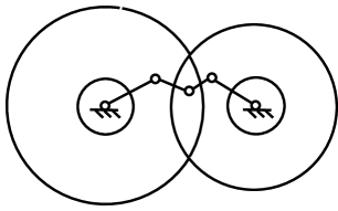
Figure 2. The lens-shaped work space ${\mathcal{W}}$ for  $\Gamma_{\operatorname{cl}}^{5}$

1.7 Remark.

The configuration spaces studied in this paper are mathematical models, which take into account only the locations of the vertices of $\Gamma$, disregarding possible intersections of the edges. In the plane, there is some justification for this, since we can allow one link to slide over another. This is why this model is commonly used (cf. [F, KM1]; but see [CDR]). However, in  ${\mathbb{R}}^{3}$   the model is not very realistic, since it disregards the fact that rigid rods cannot pass through each other.

Thus a proper treatment of configurations in  ${\mathbb{R}}^{3}$   must cut our “naive” version of  $\operatorname{Emb}^{d}({{\mathcal{T}}_{\Gamma}})$   (and thus  ${\mathcal{C}}(\Gamma)$   and  ${\mathcal{C}}_{\ast}(\Gamma)$)  along the subspace of configurations which are not embeddings of the full graph  ${\mathcal{T}}_{\Gamma}$.  The precise description of such a “realistic” configuration space  $\operatorname{Conf}({\mathcal{T}}_{\Gamma})$   is quite complicated, even at the combinatorial level, which is why we work here with  $\operatorname{Emb}^{d}({{\mathcal{T}}_{\Gamma}})$,   ${\mathcal{C}}(\Gamma)$,  and  ${\mathcal{C}}_{\ast}(\Gamma)$   as defined in §1.1-1.4. Note, however, that  ${\mathcal{C}}(\Gamma)$   has a dense open subspace  $U(\Gamma)$   consisting of embeddings of the full graph (including its edges), which may be identified with a dense open subset of  $\operatorname{Conf}({\mathcal{T}}_{\Gamma})$.  We observe that even such a model  $\operatorname{Conf}({\mathcal{T}}_{\Gamma})$   is not completely realistic, in that it disregards the thickness of the rigid rods.

Unfortunately, the generic singularities we identify here are not in  $U(\Gamma)$.  Nevertheless, in some cases at least, our method of replacing one singular configuration by another (see Section 2 below) allows us to replace the generic singularity in  ${\mathcal{C}}(\Gamma)\setminus U(\Gamma)$   with a configuration in  $U(\Gamma^{\prime})$,  for a suitable linkage  $\Gamma^{\prime}$.  See Section 5 for an example of this phenomenon (which also occurs in the $3$-dimensional version of the linkage described there).

2. Local equivalences of configuration spaces

Let $\Gamma$ and  $\Gamma^{\prime}$   be two linkages. We would like to think of points in the respective configuration spaces as being equivalent if they are both smooth, or both have “similar” singularities. Since these concepts are local, we make the following:

2.1 Definition.

Two configurations ${\mathcal{V}}$ in  ${\mathcal{C}}(\Gamma)$   and  ${\mathcal{V}}\,^{\prime}$   in  ${\mathcal{C}}(\Gamma^{\prime})$   are:

1. locally equivalent if there are neighborhoods $U$ of ${\mathcal{V}}$ in  ${\mathcal{C}}_{\ast}(\Gamma)$   and  $U^{\prime}$   of  ${\mathcal{V}}\,^{\prime}$   in  ${\mathcal{C}}_{\ast}(\Gamma^{\prime})$,  and a homeomorphism  $f:U\to U^{\prime}$   with  $f({\mathcal{V}})={\mathcal{V}}\,^{\prime}$.

2. locally product-equivalent if there are neighborhoods $W$ of ${\mathcal{V}}$ in  ${\mathcal{C}}_{\ast}(\Gamma)$   and  $W^{\prime}$   of  ${\mathcal{V}}\,^{\prime}$   in  ${\mathcal{C}}_{\ast}(\Gamma^{\prime})$   equipped with homeomorphisms  $W\cong U\times{\mathbb{R}}^{k}$   (taking ${\mathcal{V}}$ to  $({\mathcal{V}}_{0},\mathbf{x})$)  and  $W^{\prime}\cong U^{\prime}\times{\mathbb{R}}^{m}$   (taking  ${\mathcal{V}}\,^{\prime}$   to  $({\mathcal{V}}\,^{\prime}_{0},\mathbf{y})$),  as well as a homeomorphism  $f:U\to U^{\prime}$   with  $f({\mathcal{V}}_{0})={\mathcal{V}}\,^{\prime}_{0}$.

See [KM3] for other formulations of this and similar notions.

Evidently, any two smooth configurations in any two configuration spaces are locally product-equivalent.

In the next section we decompose our configuration spaces into simpler factors (locally), gluing them along appropriate work maps. The singularities of the configuration spaces translate into work singularities on the factors, so we need an analogous notion of work maps being locally equivalent (at smooth configurations), or locally equivalent up to a Euclidean factor:

2.2 Definition.

If  $i:\Delta\hookrightarrow\Gamma$   and  $i^{\prime}:\Delta\hookrightarrow\Gamma^{\prime}$   are inclusions of a common rigid sub-mechanism $\Delta$ (usually a single point) in two distinct linkages, and  ${\mathcal{V}}\in{\mathcal{C}}_{\ast}(\Gamma)$,   ${\mathcal{V}}\,^{\prime}\in{\mathcal{C}}_{\ast}(\Gamma^{\prime})$   are two smooth configurations, we say that  $i^{\ast}$   and  $(i^{\prime})^{\ast}$   are

1. work-equivalent at  $({\mathcal{V}},{\mathcal{V}}\,^{\prime})$   if there are neighborhoods $U$ of ${\mathcal{V}}$,  $U^{\prime}$   of  ${\mathcal{V}}\,^{\prime}$,  and $W$ of  $i^{\ast}({\mathcal{V}})=(i^{\prime})^{\ast}({\mathcal{V}}\,^{\prime})$,  and a diffeomorphism $f$ making the following diagram commute:

   (2.3)

2. $S$-equivalent at  $({\mathcal{V}},{\mathcal{V}}\,^{\prime})$   if there are neighborhoods  $W\cong U\times{\mathbb{R}}^{k}$   of ${\mathcal{V}}$ and  $W^{\prime}\cong U^{\prime}\times{\mathbb{R}}^{m}$   of  ${\mathcal{V}}\,^{\prime}$   and a homeomorphism  $f:U\to U^{\prime}$   as in §2.1(b) above, such  $i^{\ast}$   factors through the projection  $\pi:W\to U$   and  $(i^{\prime})^{\ast}$   factors through  $\pi^{\prime}:W^{\prime}\to U^{\prime}$   in such a way that the diagram analogous to  (2.3)   commutes.

An important example of these notions is provided by the following simple mechanism:

2.4 Definition.

An open $k$-chain is a linkage  $\Gamma_{\operatorname{op}}^{k}$,  where  ${\mathcal{T}}_{\Gamma}$   is a connected linear graph with  $k+1$   vertices (where all but the endpoints  $\mathbf{x}^{({0})}$   and  $\mathbf{x}^{({k})}$   are of valency $2$), with lengths  $(\ell_{1},\dotsc,\ell_{k})$.  See Figure 3 below. It is natural to choose the base-point  $\mathbf{x}_{\star}:=\mathbf{x}^{({0})}$   (fixed at the origin, say) to define the pointed configuration space  ${\mathcal{C}}_{\ast}(\Gamma_{\operatorname{op}}^{k})$,  and  $\mathbf{x}_{e}:=\mathbf{x}^{({k})}$   as end-effector.

The resulting workspace ${\mathcal{W}}$ is  $S^{d-1}\times[m,M]$,  for fixed  $0<m<M$,  where  $m=\min\{|\sum_{i=1}^{k}\pm\ell_{i}|\}$   and  $M=\sum_{i=1}^{k}\ell_{i}$   are respectively the minimal and maximal possible distances of  $\mathbf{x}_{e}$   from  $\mathbf{x}_{\star}$.  The spherical (or polar) coordinate  $\theta\in S^{d-1}$   is the direction of the vector  $\vec{\mathbf{v}}=\mathbf{x}_{e}-\mathbf{x}_{\star}$.

A closed  ($k+1$)-chain is a linkage  $\Gamma_{\operatorname{cl}}^{k+1}$,  where  ${\mathcal{T}}_{\Gamma}$   is a cycle with  $k+1$   vertices (of valency $2$), having lengths  $\ell_{1}=|\mathbf{x}^{({1})}-\mathbf{x}^{({0})}|,\ell_{2}=|\mathbf{x}^{({2})}-\mathbf{x}^{({1})}|,\dotsc,\ell_{k+1}=|\mathbf{x}^{({0})}-\mathbf{x}^{({k})}|$   (see Figure 1).

A prismatic closed  ($k+1$)-chain  $\Gamma_{\operatorname{pcl}}^{k+1}$   has the same  ${\mathcal{T}}_{\Gamma}$,  with lengths  $(\ell_{1},\dotsc,\ell_{k})$   as for  $\Gamma_{\operatorname{cl}}^{k+1}$,  but with the last link prismatic  –  that is, the length  $\ell=|\mathbf{x}^{({0})}-\mathbf{x}^{({k})}|$   varies in the range  $m\leq\ell\leq M$.

2.5 Lemma ([G]).

The work map $\psi$ of an open chain is a submersion, unless  ${\mathcal{V}}$   is aligned (that is, all links have a common direction vector $\vec{\mathbf{w}}$ in  ${\mathbb{R}}^{d}$   at ${\mathcal{V}}$). In this case the  $(d-1)$-dimensional subspace  $\operatorname{Im}(\operatorname{d}\!\psi)_{{\mathcal{V}}}$   is orthogonal to $\vec{\mathbf{w}}$.

Clearly the configuration spaces of an open $k$-chain and the corresponding prismatic closed  ($k+1$)-chain are isomorphic. However, the following result will be useful in understanding the work map singularities of an open chain, by allowing us to disregard its  ($d-1$)-dimensional non-singular direction.

2.6 Proposition.

If  $\Gamma_{\operatorname{op}}^{k}$   is an open $k$-chain with links  $(\ell_{1},\dotsc,\ell_{k})$,  then the pointed configuration space ${\mathcal{C}}_{\ast}(\Gamma_{\operatorname{op}}^{k})$   is $S$-equivalent at any configuration ${\mathcal{V}}$ to the reduced configuration space  $\widehat{{\mathcal{C}}}_{\ast}(\Gamma_{\operatorname{pcl}}^{k+1})$   of a closed prismatic  ($k+1$)-chain.

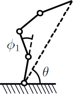
Figure 3. Coordinates for the open chain

Proof.

We may choose  $(\theta,\phi_{1},\dotsc,\phi_{k-1})\in(S^{d-1})^{k}$   as local coordinates for the smooth configuration space  ${\mathcal{C}}_{\ast}(\Gamma_{\operatorname{op}}^{k})$   near ${\mathcal{V}}$, where  $\phi_{i}$   is the spherical angle between the vectors  $\mathbf{x}^{({i-1})}\mathbf{x}^{({i})}$   and  $\mathbf{x}^{({i})}\mathbf{x}^{({i+1})}$   (see Figure 3), and $\theta$ is as in §2.4 (for  $\vec{\mathbf{v}}\neq\vec{\mathbf{0}}$).

Thus in a coordinate neighborhood  $U\cong{\mathbb{R}}^{k(d-1)}$   of ${\mathcal{V}}$ the work map  $i^{\ast}:U\to{\mathbb{R}}^{d-1}\times[m,M]$   factors as  $(\pi_{\theta},\rho)$,  where  $\pi_{\theta}(\theta,\phi_{1},\dotsc,\phi_{k-1})=\theta$   is the projection, and  $\rho(\theta,\phi_{1},\dotsc,\phi_{k-1})=\|\mathbf{x}^{({k})}-\mathbf{x}^{({0})}\|\in[m,M]$.

Now for each  $\ell\in[m,M]$,  the fiber  $\rho^{-1}(\ell)$   is diffeomorphic to the configuration space  ${\mathcal{C}}_{\ast}(\Gamma_{\operatorname{cl}}^{k+1})$   of a closed chain having  $k+1$   links of lengths  $(\ell_{1},\dotsc,\ell_{k},\ell)$.  As in §1.4, we have  ${\mathcal{C}}_{\ast}(\Gamma_{\operatorname{cl}}^{k+1})\cong S^{d-1}\times\widehat{{\mathcal{C}}}_{\ast}(\Gamma_{\operatorname{cl}}^{k+1})$,  so  ${\mathcal{C}}_{\ast}(\Gamma_{\operatorname{cl}}^{k+1})$   is locally product-equivalent to  $\widehat{{\mathcal{C}}}_{\ast}(\Gamma_{\operatorname{cl}}^{k+1})$, and in fact  ${\mathcal{C}}_{\ast}(\Gamma_{\operatorname{cl}}^{k+1})$   is $S$-equivalent to  $\widehat{{\mathcal{C}}}_{\ast}(\Gamma_{\operatorname{cl}}^{k+1})$   with respect to  $\Delta=\{\mathbf{x}^{({k})}\}$.  As $\ell$ varies, we obtain the mechanism  $\Gamma_{\operatorname{pcl}}^{k+1}$.

If  $\vec{\mathbf{v}}:=\mathbf{x}_{e}-\mathbf{x}_{\star}$   vanishes at ${\mathcal{V}}$, but ${\mathcal{V}}$ is not aligned, then the work map $\psi$ is a submersion at ${\mathcal{V}}$, and the same holds for  ${\mathcal{C}}_{\ast}(\Gamma_{\operatorname{pcl}}^{k+1})$,  so they are $S$-equivalent. If  $\vec{\mathbf{v}}=\mathbf{z}$   at ${\mathcal{V}}$ and ${\mathcal{V}}$ is aligned, choose the coordinate $\theta$ be the direction of the alignment vector $\vec{\mathbf{w}}$. ∎

2.7.

Decomposing the work map.

Consider an arbitrary mechanism $\Gamma$ with base point  $\mathbf{x}_{\star}$   and work map  $\psi:{\mathcal{C}}_{\ast}(\Gamma)\to{\mathbb{R}}^{d}$   for the end-effector  $\mathbf{x}_{e}$.  Note that  ${\mathcal{C}}_{\ast}(\Gamma)$   is locally diffeomorphic to the product  $S^{d-1}\times\widehat{{\mathcal{C}}}_{\ast}(\Gamma)$   (§1.4), since the bundle  $\widehat{{\mathcal{C}}}_{\ast}(\Gamma)\hookrightarrow{\mathcal{C}}_{\ast}(\Gamma)\to S^{d-1}$   (for  $\vec{\mathbf{v}}:=\mathbf{x}_{e}-\mathbf{x}_{\star}\in S^{d-1}$)  is locally trivial (assuming $\vec{\mathbf{v}}$ does not vanish). If we choose local spherical coordinates  $S^{d-1}\times{\mathbb{R}}_{+}$   for the work space  ${\mathcal{W}}\subseteq{\mathcal{C}}(\Delta)\subseteq{\mathbb{R}}^{d}$,  the work map  $\psi:{\mathcal{C}}_{\ast}(\Gamma)\to{\mathcal{W}}\subseteq S^{d-1}\times{\mathbb{R}}_{+}$   may be written locally in the form

(2.8) $${}\psi=\operatorname{Id}_{S^{d-1}}\times\tilde{\psi}:S^{d-1}\times\widehat{{\mathcal{C}}}_{\ast}~{}\to~{}S^{d-1}\times{\mathbb{R}}_{+}$$

for some smooth function  $\tilde{\psi}:\widehat{{\mathcal{C}}}_{\ast}\to{\mathbb{R}}_{+}$   (which is the work function for the associated reduced configuration space). Note that the derivative of the work function $\psi$ may thus be written in the form:

(2.9) $${}(\operatorname{d}\!\psi)_{(\vec{\mathbf{v}},\hat{{\mathcal{V}}})}~{}=~{}\left(\begin{array}[]{ll}I_{d-1}&\mathbf{0}\\ \mathbf{0}&(\nabla\tilde{\psi})_{\hat{{\mathcal{V}}}}\end{array}\right).$$

which shows that  $\operatorname{d}\!\psi$   has rank $d$ or  $d-1$.

2.10 Proposition.

If  ${\mathcal{V}}=(\hat{{\mathcal{V}}},{\mathcal{V}}^{\prime})\in{\mathcal{C}}_{\ast}(\Gamma)$   is a smooth configuration for a mechanism $\Gamma$ with work function  $\psi=\operatorname{Id}_{S^{d-1}}\times\tilde{\psi}$   as in  (2.8),  with  $\mathbf{x}_{e}\neq\mathbf{x}_{\star}$,  and $\hat{{\mathcal{V}}}$ is a non-degenerate singular point of $\tilde{\psi}$, then  ${\mathcal{C}}_{\ast}(\Gamma)$   is $S$-equivalent at ${\mathcal{V}}$ to an aligned configuration of an open $n$-chain for some  $n\geq 1$.

Proof.

By the Morse Lemma (cf. [Ma, Theorem 2.16]) we may choose local coordinates  $\vec{\mathbf{t}}=(t_{1},\dotsc,t_{k-d+1})$   for  $\widehat{{\mathcal{C}}}_{\ast}(\Gamma)$   near $\hat{{\mathcal{V}}}$ (where  $k=\dim{\mathcal{C}}_{\ast}(\Gamma)$),  so that $\tilde{\psi}$ has the form

(2.11) $${}\tilde{\psi}(\vec{\mathbf{t}})=a_{0}+\sum_{i=1}^{j}t_{i}^{2}-\sum_{i=j+1}^{k-d+1}t_{i}^{2}~{}.$$

On the other hand, by Proposition 2.6 the configuration space  ${\mathcal{C}}_{\ast}(\Gamma_{\operatorname{op}}^{n})$   for an open $n$-chain at any configuration  ${\mathcal{V}}^{({n})}$   is $S$-equivalent to the reduced configuration space  $\widehat{{\mathcal{C}}}_{\ast}(\Gamma_{\operatorname{pcl}}^{n+1})$   at some configuration  $\hat{{\mathcal{V}}}^{({n+1})}$,  where  $\Gamma_{\operatorname{pcl}}^{n+1}$   is a prismatic closed  ($n+1$)-chain. The reduced work map

$$\hat{\phi}:\widehat{{\mathcal{C}}}_{\ast}(\Gamma_{\operatorname{pcl}}^{n+1})\to\gamma\subseteq{\mathcal{W}}\subseteq{\mathbb{R}}^{d}$$

assigns to each  $\hat{{\mathcal{V}}}\in\widehat{{\mathcal{C}}}_{\ast}(\Gamma_{\operatorname{pcl}}^{n+1})$   the length of the variable link (with  $\gamma\cong[m,M]$,  the segment of possible lengths).

As shown in [MT, Theorem 5.4], $\hat{\phi}$ is a Morse function, having (non-degenerate) singular points precisely at the aligned configurations  $\hat{{\mathcal{V}}}^{({n+1})}$   of the closed chain  $\Gamma_{\operatorname{pcl}}^{n+1}$.  Although Milgram and Trinkle do not calculate the index of $\hat{\phi}$ at  $\hat{{\mathcal{V}}}^{({n+1})}$,  their computation of the Hessian of $\hat{\phi}$ in [MT, Key Example, p. 255], combined with Farber’s proof of [F, Lemma 1.4] for the planar case, show that this index is equal to  $n-k$,  where $k$ is the number of forward-pointing links in the configuration  $\hat{{\mathcal{V}}}^{({n+1})}$.  Thus by the Morse Lemma again we may choose an aligned configuration  $\hat{{\mathcal{V}}}^{({n+1})}$   and local coordinates in  $\widehat{{\mathcal{C}}}_{\ast}(\Gamma_{\operatorname{pcl}}^{n+1})$   around it so that $\hat{\phi}$ too has the form  (2.11),  and thus  ${\mathcal{C}}_{\ast}(\Gamma)$   is $S$-equivalent at ${\mathcal{V}}$ to  $\widehat{{\mathcal{C}}}_{\ast}(\Gamma_{\operatorname{pcl}}^{n+1})$   at  $\hat{{\mathcal{V}}}^{({n+1})}$.  By Proposition 2.6 it is then readily seen to be $S$-equivalent to  ${\mathcal{C}}_{\ast}(\Gamma_{\operatorname{op}}^{n})$   at the corresponding aligned open-chain configuration  ${\mathcal{V}}^{({n})}$.  ∎

3. Pullbacks of configuration spaces

We now describe a procedure for viewing the configuration space of an arbitrary linkage $\Gamma$ as a pullback, obtained by decomposing $\Gamma$ into two simpler sub-mechanisms. The basic idea is a familiar one  –  see, e.g., [MT].

3.1.

Pullbacks. Let  $\Gamma_{\operatorname{op}}^{k}$   denote an open chain which is a sub-mechanism of $\Gamma$ (cf. §2.4), and let  $\Gamma^{\prime}$   denote the mechanism obtained from $\Gamma$ by omitting the $k$ links of  $\Gamma_{\operatorname{op}}^{k}$   (and all vertices but  $\mathbf{x}^{({0})}$   and  $\mathbf{x}^{({k})}$).  For simplicity we choose  $\mathbf{x}_{\star}:=\mathbf{x}^{({0})}$   as the common base-point of $\Gamma$,  $\Gamma_{\operatorname{op}}^{k}$,  and  $\Gamma^{\prime}$,  and  $\mathbf{x}_{e}:=\mathbf{x}^{({k})}$   as the common end-effector of  $\Gamma_{\operatorname{op}}^{k}$   and  $\Gamma^{\prime}$.  See Figure 4.

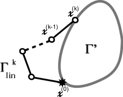
Figure 4. Decomposing $\Gamma$ into two sub-mechanisms

The work space of both mechanisms  $\Gamma^{\prime}$   and  $\Gamma_{\operatorname{op}}^{k}$   (i.e., the set of possible locations for  $\mathbf{x}_{e}$)  is contained in  ${\mathbb{R}}^{d}$,  and we have work maps  $\psi:{\mathcal{C}}_{\ast}(\Gamma^{\prime})\to{\mathbb{R}}^{d}$   and  $\phi:{\mathcal{C}}_{\ast}(\Gamma_{\operatorname{op}}^{k})\to{\mathbb{R}}^{d}$   which associate to each configuration the location of  $\mathbf{x}_{e}$.

Note that the pointed configuration space  ${\mathcal{C}}_{\ast}(\Gamma_{\operatorname{op}}^{k})$   is a manifold (diffeomorphic to  $(S^{d-1})^{k}$)  with a natural embedding  $i:{\mathcal{C}}_{\ast}(\Gamma_{\operatorname{op}}^{k})\hookrightarrow{\mathbb{R}}^{kd}$,  and similarly  $j:{\mathcal{C}}_{\ast}(\Gamma^{\prime})\to{\mathbb{R}}^{M}$   for a suitable Euclidean space  ${\mathbb{R}}^{M}$.  This can be done, for example, by using the position coordinates in  ${\mathbb{R}}^{d}$   for every vertex in $\Gamma$.

Let  $X:={\mathcal{C}}_{\ast}(\Gamma_{\operatorname{op}}^{k})\times{\mathbb{R}}^{M}$   and  $Y:={\mathbb{R}}^{d}\times{\mathbb{R}}^{M}$,  and define  $h:X\to Y$   to be the product map  $\phi\times\operatorname{Id}_{{\mathbb{R}}^{M}}$   and  $g:{\mathcal{C}}_{\ast}(\Gamma^{\prime})\to Y$   to be  $(\psi,j)$,  so that $g$ is an embedding of  ${\mathcal{C}}_{\ast}(\Gamma^{\prime})$   as a submanifold in $Y$. Since we have a pullback square:

(3.2)

${\mathcal{C}}_{\ast}(\Gamma)$   may be identified with the preimage of the subspace  ${\mathcal{C}}_{\ast}(\Gamma^{\prime})\subseteq Y$   under $h$.

Let  ${\mathcal{V}}\,^{\prime}\in{\mathcal{C}}_{\ast}(\Gamma^{\prime})$   and  ${\mathcal{V}}^{({k})}\in{\mathcal{C}}_{\ast}(\Gamma_{\operatorname{op}}^{k})$   be matching configurations with  $\psi({\mathcal{V}}\,^{\prime})=\phi({\mathcal{V}}^{({k})})$,  and let  $\mathbf{x}\in X$   be the configuration  $({\mathcal{V}}^{({k})},j({\mathcal{V}}\,^{\prime}))$,  so that  $h(\mathbf{x})=g({\mathcal{V}}\,^{\prime})$:

(3.3)

We want to know if the point  ${\mathcal{V}}\in{\mathcal{C}}_{\ast}(\Gamma)$   defined by  $({\mathcal{V}}\,^{\prime},{\mathcal{V}}^{({k})})$   is singular. By [Hi, I, Theorem 3.3], ${\mathcal{V}}$ is smooth if  $h\pitchfork{\mathcal{C}}_{\ast}(\Gamma^{\prime})$    –  i.e., $h$ is locally transverse to  ${\mathcal{C}}_{\ast}(\Gamma^{\prime})$   at the points  $\mathbf{x}\in X$   and  ${\mathcal{V}}\,^{\prime}\in{\mathcal{C}}_{\ast}(\Gamma^{\prime})$,  which means that  $\operatorname{Im}\operatorname{dh}_{\mathbf{x}}~{}+~{}T_{{\mathcal{V}}\,^{\prime}}({\mathcal{C}}_{\ast}(\Gamma^{\prime}))~{}=~{}T_{{\mathcal{V}}\,^{\prime}}(Y)~{}=~{}{\mathbb{R}}^{d}\times{\mathbb{R}}^{M}$.

Since  $\operatorname{Id}_{{\mathbb{R}}^{M}}$   is onto, this is equivalent to:

(3.4) $${}\operatorname{Im}(\operatorname{d}\!\phi)_{{\mathcal{V}}^{({k})}}~{}+~{}\operatorname{Im}(\operatorname{d}\!\psi)_{{\mathcal{V}}\,^{\prime}}~{}=~{}{\mathbb{R}}^{d}$$

3.5.

Generic singularities in pullbacks. Clearly, the failure of  (3.4)   is a necessary condition for  ${\mathcal{V}}=({\mathcal{V}}\,^{\prime},{\mathcal{V}}^{({k})})$   to be singular in  ${\mathcal{C}}_{\ast}(\Gamma)$.  Note that if  (3.4)   does not hold, then neither  $(\operatorname{d}\!\phi)_{{\mathcal{V}}^{({k})}_{n}}$   nor  $(\operatorname{d}\!\psi)_{{\mathcal{V}}\,^{\prime}_{n}}$   is onto  ${\mathbb{R}}^{d}$.  By Lemma 2.5, the first implies that the configuration  ${\mathcal{V}}^{({k})}_{n}$   for the open chain  $\Gamma_{\operatorname{op}}^{k}$   must be aligned, while the second implies that  $(\operatorname{d}\!\psi)_{{\mathcal{V}}\,^{\prime}_{n}}$   is of rank $<d$.

3.6 Definition.

Given a pullback diagram as in  (3.2),  a configuration  $({\mathcal{V}}\,^{\prime},{\mathcal{V}}^{({k})})\in{\mathcal{C}}_{\ast}(\Gamma)\subseteq{\mathcal{C}}_{\ast}(\Gamma^{\prime})\times{\mathcal{C}}_{\ast}(\Gamma_{\operatorname{op}}^{k})$   will be called generically non-transverse if  $\hat{{\mathcal{V}}}^{\prime}$   is a non-degenerate singular point of $\tilde{\psi}$, and  $\mathbf{x}^{({0})}\neq\mathbf{x}^{({k})}$.

3.7 Remark.

Note that since  $\tilde{\psi}:\widehat{{\mathcal{C}}}^{\prime}_{\ast}\to{\mathbb{R}}_{+}$   is an algebraic function, generically it will be a Morse function, so any singular point  $\hat{{\mathcal{V}}}^{\prime}$   is non-degenerate. Likewise, in the moduli space  $\Lambda={\mathbb{R}}^{k}_{+}$   for open $k$-chains, the subspace of moduli $\lambda$ for which  $\Gamma_{\operatorname{op}}^{k}$   has no aligned configurations with  $\mathbf{x}^{({0})}=\mathbf{x}^{({k})}$   is Zariski open in $\Lambda$. Thus among the potentially singular configurations of  ${\mathcal{C}}_{\ast}(\Gamma)$   (i.e., those for which  (3.4)   fails), the generically non-transverse ones are indeed generic.

3.8 Proposition.

Given a pullback diagram  (3.2),  any generically non-transverse configuration  $({\mathcal{V}}\,^{\prime},{\mathcal{V}}^{({k})})$   is the product of a Euclidean space with a cone on a homogeneous quadratic hypersurface, so in particular it is a topological singularity of  ${\mathcal{C}}_{\ast}(\Gamma)$.

Proof.

Since  $\hat{{\mathcal{V}}}^{\prime}$   is a non-degenerate singular point of $\tilde{\psi}$, by Proposition 2.10 the work map  $\psi:{\mathcal{C}}_{\ast}(\Gamma^{\prime})\to{\mathcal{W}}\subseteq{\mathbb{R}}^{d}$   is work-equivalent to the work map $\eta$ of an open chain  $\Gamma_{\operatorname{op}}^{n}$   at some aligned configuration  ${\mathcal{V}}^{({n})}$.  Thus the pullback diagram  (3.2)   may be replaced by one of the form

(3.9)

so that ${\mathcal{C}}$ itself is $S$-equivalent at  $({\mathcal{V}}^{({k})},{\mathcal{V}}^{({n})})$   to the configuration space of a closed chain with  $(n+k)$   links at an aligned configuration (since $\phi$ and $\eta$ were non-transverse). This is known to be the cone on a homogeneous quadratic hypersurface, by [F, Theorem 1.6] and [KM2, Theorem 2.6], so it is topologically singular. ∎

4. Inductive construction of configuration spaces

We now define an inductive process for studying the local behavior of a configuration ${\mathcal{V}}$ of a linkage $\Gamma$. This consists of successively discarding open chains of $\Gamma$ while preserving the local structure.

4.1.

The inductive procedure. We saw in §3.1 how removing an open chain sub-mechanism from $\Gamma$ allows one to describe the configuration space  ${\mathcal{C}}_{\ast}(\Gamma)$   as a pullback of two configuration spaces  ${\mathcal{C}}_{\ast}(\Gamma_{\operatorname{op}}^{k})$   and  ${\mathcal{C}}_{\ast}(\Gamma^{\prime})$,  where the first is completely understood, and the second is simpler than the original  ${\mathcal{C}}_{\ast}(\Gamma)$.

This idea may now be applied again to  ${\mathcal{C}}_{\ast}(\Gamma^{\prime})$:  by repeatedly discarding (or adding) open chain sub-mechanisms, we construct a sequence of pullbacks

(4.2)

for  $1\leq n<M$,  where each  $\Gamma_{n-1}$   is a sub-mechanism of  $\Gamma_{n}$,  with  $\Gamma=\Gamma_{M}$,  and  $\Lambda_{n}$   is an open chain in  ${\mathbb{R}}^{d}$   (so  ${\mathcal{C}}(\Lambda_{n})$   is a product of  $(d-1)$ -spheres). The maps  $\psi_{n}$   and  $\phi_{n}$  are work maps for the common endpoint of  $\Gamma_{n}$   and  $\Lambda_{n}$.

Each configuration ${\mathcal{V}}$ for $\Gamma$ determines a sequence of pairs  ${\mathcal{V}}\,^{\prime}_{n+1}=({\mathcal{V}}\,^{\prime}_{n},{\mathcal{V}}^{({k})}_{n})$   in  ${\mathcal{C}}(\Gamma_{n+1})$,  as in  (4.2),  where  ${\mathcal{V}}^{({k})}_{n}$   is necessarily a smooth point of  ${\mathcal{C}}(\Lambda_{n})$.  Evidently, if  ${\mathcal{V}}\,^{\prime}_{n}$   is a smooth point of  ${\mathcal{C}}(\Gamma_{n})$,   ${\mathcal{V}}\,^{\prime}_{n+1}$   will be, too, if  (3.4)   holds.

4.3 Remark.

Note that there is usually more than one way to decompose a given linkage $\Gamma$ as in §3.1, so the full inductive process described above is actually encoded by an (inverted) rooted tree, with varying degrees at each node (and the root at $\Gamma$ itself). Any rooted branch  $(\Gamma_{n},\Lambda_{n})_{n=k}^{M-1}$    ($\Gamma_{M}=\Gamma$)   of this tree will be called a decomposition of $\Gamma$.

This flexibility can be very useful in applying the inductive procedure (see §4.5 below for an example).

4.4.

Generic singularities in  ${\mathcal{C}}_{\ast}(\Gamma)$. Our goal is to use this procedure to study singular configurations of  ${\mathcal{C}}(\Gamma)$.  Here we start with the simplest case, which is also the generic form of singularities in configuration spaces, as we shall see below.

Thus we assume by induction that  ${\mathcal{V}}\,^{\prime}_{n}$   is a smooth configuration, but  (3.4)   fails. Our goal is to analyze this failure in the generic case, and then show that in this case  ${\mathcal{V}}\,^{\prime}_{n+1}$   is a singular point. Eventually, we would like to use this to deduce that the original configuration ${\mathcal{V}}$ is singular, too.

In §3.5, we saw how to identify positively the generic singularities appearing in one step in the inductive process of §4.1, defined by a pullback diagram  (4.2):  namely, if  ${\mathcal{V}}\,^{\prime}_{n+1}\in{\mathcal{C}}(\Gamma_{n+1})$   is defined by a pair of smooth configurations  $({\mathcal{V}}\,^{\prime}_{n},{\mathcal{V}}^{({k})}_{n})$,  but  (3.4)   fails, then generically at least,  ${\mathcal{V}}\,^{\prime}_{n+1}$   is a topological singularity. However, this does not yet guarantee that the corresponding configuration ${\mathcal{V}}$ in  ${\mathcal{C}}_{\ast}(\Gamma)$   itself is singular (unless  $\Gamma=\Gamma_{n+1}$,  of course).

4.5 Example.

Let  $\Gamma_{\operatorname{cl}}^{4}$   be a planar closed $4$-chain with links of lengths  $\ell^{({1})},\ell^{({2})},\ell^{({3})}$,  and  $\ell^{({4})}$.  See Figure 5.

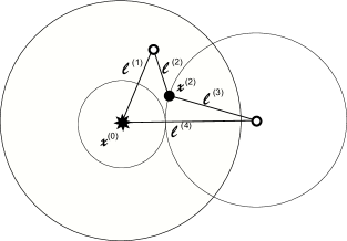
Figure 5. Workspace for the point  $\mathbf{x}^{({2})}$   of a closed $4$-chain

Generically,  $\widehat{{\mathcal{C}}}_{\ast}(\Gamma_{\operatorname{cl}}^{4})$   is a smooth $1$-dimensional manifold, with local parameter given by $\theta$ (the angle between  $\mathbf{v}^{({1})}$   and  $\mathbf{v}^{({3})}$,  say). However, if  $\ell^{({1})}+\ell^{({3})}=\ell^{({2})}+\ell^{({4})}$,  then  $\widehat{{\mathcal{C}}}_{\ast}(\Gamma_{\operatorname{cl}}^{4})$   has a topological singularity  –  a node  –  at the aligned configuration $\hat{{\mathcal{V}}}$ where the links  $\mathbf{v}^{({1})}$   and  $\mathbf{v}^{({3})}$   face right, say, and  $\mathbf{v}^{({2})}$   and  $\mathbf{v}^{({4})}$   face left (see [F, Theorem 1.6]). In fact, if there are no further relations among  $\ell^{({1})},\dotsc,\ell^{({4})}$,  this is the only singularity, and  $\widehat{{\mathcal{C}}}_{\ast}(\Gamma_{\operatorname{cl}}^{4})$   is a figure eight (the one point union of two circles). We can think of  $\Gamma_{\operatorname{cl}}^{4}$   as being decomposed into two sub-mechanisms  $\Gamma^{\prime}$   and  $\Gamma^{\prime\prime}$,  each an open $2$-chain:  $\Gamma^{\prime}$   consisting of  $\mathbf{v}^{({1})}$   and  $\mathbf{v}^{({2})}$,  and  $\Gamma^{\prime\prime}$   of  $\mathbf{v}^{({3})}$   and  $\mathbf{v}^{({4})}$.  Note that  $\hat{{\mathcal{V}}}:=({\mathcal{V}}\,^{\prime},{\mathcal{V}}\,^{\prime\prime})$,  where  ${\mathcal{V}}\,^{\prime}$   and  ${\mathcal{V}}\,^{\prime\prime}$   are both aligned.

In this case we can describe  ${\mathcal{C}}_{\ast}(\Gamma_{\operatorname{cl}}^{4})$   explicitly in terms of the work map  $\phi:{\mathcal{C}}_{\ast}(\Gamma_{\operatorname{cl}}^{4})\to{\mathbb{R}}^{2}$   (for the vertex  $\mathbf{x}_{e}:=\mathbf{x}^{({2})}$),  which is a four-fold covering map at all points but ${\mathcal{V}}$: in a punctured neighborhood of ${\mathcal{V}}$, neither  ${\mathcal{V}}\,^{\prime}$   nor  ${\mathcal{V}}\,^{\prime\prime}$   can be aligned, and each independently can have an “elbow up” ($+$) or “elbow down” ($-$) position, which together provide the four discrete configurations corresponding to a single value of $\phi$. In  $\widehat{{\mathcal{C}}}_{\ast}(\Gamma_{\operatorname{cl}}^{4})$,  taken together, these give four different branches of the curve (parameterized by $\theta$)  –  which coincide at ${\mathcal{V}}$. See Figure 6.

Figure 6. The four branches of  $\widehat{{\mathcal{C}}}_{\ast}(\Gamma_{\operatorname{cl}}^{4})$

Now assume given a linkage $\Gamma$ in which  $\Gamma_{2}=\Gamma_{\operatorname{cl}}^{4}$   as above (with  $\ell^{({1})}+\ell^{({3})}=\ell^{({2})}+\ell^{({4})}$).  Assume that to obtain  $\Gamma_{3}$   we add an open $2$-chain  $\Lambda_{2}\Gamma_{\operatorname{op}}^{2}$,  having vertices  $\mathbf{x}^{({0})}$,   $\mathbf{x}^{({3})}$,  and  $\mathbf{x}^{({4})}$,  with  $\|\mathbf{x}^{({0})}\mathbf{x}^{({4})}\|=\ell^{({5})}$   and  $\|\mathbf{x}^{({3})}\mathbf{x}^{({4})}\|=\ell^{({6})}$.  We therefore now have a rigid triangle  $\triangle\mathbf{x}^{({0})}\mathbf{x}^{({3})}\mathbf{x}^{({4})}$   (with  $\mathbf{x}^{({4})}$   in “elbow up” or “elbow down” position relative to the edge  $\mathbf{x}^{({0})}\mathbf{x}^{({3})}$).  Thus  ${\mathcal{C}}_{\ast}(\Gamma_{3})={\mathcal{C}}_{\ast}(\Gamma_{2})\times\{\pm 1\}$,  and the singularity at  ${\mathcal{V}}\,^{\prime}_{2}:=\hat{{\mathcal{V}}}$   is unaffected.

In the last stage  $\Gamma=\Gamma_{4}$   is obtained by adding another open $2$-chain  $\Lambda_{3}:=\Gamma_{\operatorname{op}}^{2}$   with one new vertex  $\mathbf{x}^{({5})}$,   $\|\mathbf{x}^{({4})}\mathbf{x}^{({5})}\|=\ell^{({7})}$   and  $\|\mathbf{x}^{({5})}\mathbf{x}^{({1})}\|=\ell^{({8})}$.  We require the configuration  ${\mathcal{V}}^{({2})}_{2}$   of  $\Lambda_{3}$   in which  $\mathbf{x}^{({1})}$,   $\mathbf{x}^{({4})}$,  and  $\mathbf{x}^{({5})}$   are aligned to coincide with the aligned configuration  ${\mathcal{V}}\,^{\prime}_{2}=\hat{{\mathcal{V}}}$   of  $\Gamma_{2}$   (and thus  ${\mathcal{V}}\,^{\prime}_{3}=({\mathcal{V}}\,^{\prime}_{2},+)$   of  $\Gamma_{3}$).

The effect of adding  $\Lambda_{3}$   is to prevent the open chain  $\Gamma^{\prime}=\mathbf{x}^{({0})}\mathbf{x}^{({1})}\mathbf{x}^{({2})}$   from ever being in an “elbow down” position, thus eliminating two of the four branches of  $\widehat{{\mathcal{C}}}_{\ast}(\Gamma_{\operatorname{cl}}^{4})$   (see Figure 6), so  ${\mathcal{V}}:=({\mathcal{V}}\,^{\prime}_{3},{\mathcal{V}}^{({2})}_{2})$   (which reduces to $\hat{{\mathcal{V}}}$ in  ${\mathcal{C}}_{\ast}(\Gamma_{2})$)  is not singular in  ${\mathcal{C}}_{\ast}(\Gamma)$.

To show that this is indeed so, consider an alternative decomposition of $\Gamma$ (see Remark 4.3 above), in which we start with the closed $5$-chain  $\Gamma_{1}=\mathbf{x}^{({4})}\mathbf{x}^{({5})}\mathbf{x}^{({1})}\mathbf{x}^{({2})}\mathbf{x}^{({3})}$,  with base point  $\mathbf{x}^{({3})}$.  See Figure 7. Note that  ${\mathcal{V}}\,^{\prime}_{1}$   corresponding to $\hat{{\mathcal{V}}}$ is non-singular in  ${\mathcal{C}}_{\ast}(\Gamma_{1})$.  When we add the open $2$-chain  $\Lambda_{1}=\mathbf{x}^{({3})}\mathbf{x}^{({0})}\mathbf{x}^{({1})}$,  we see that the configuration  ${\mathcal{V}}^{({k})}_{1}$   corresponding to ${\mathcal{V}}$ is aligned, but since the work map  $\phi_{1}:{\mathcal{C}}_{\ast}(\Gamma_{1})\to{\mathbb{R}}^{2}$   determined by the work point  $\mathbf{x}^{({1})}$   is a submersion at  ${\mathcal{V}}\,^{\prime}_{1}$,  condition  (3.4)   holds at  ${\mathcal{V}}=({\mathcal{V}}\,^{\prime}_{1},{\mathcal{V}}^{({k})}_{1})$,  so ${\mathcal{V}}$ is smooth.

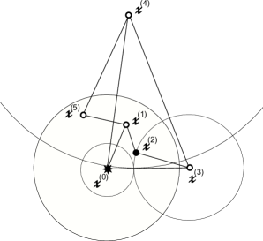
Figure 7. An alternative decomposition of $\Gamma$

4.6.

Singularities in the inductive process. In Example 4.5 we saw that a singularity appearing at one stage in the inductive process described in §4.1 can disappear at a later stage. However, in that case the reason was that the aligned configuration  ${\mathcal{V}}^{({2})}_{2}$   of  $\Lambda_{2}=\Gamma_{\operatorname{op}}^{2}$   matched up in  (4.2)   with the aligned configuration  ${\mathcal{V}}\,^{\prime}_{3}$   of  $\Gamma_{3}$.

4.7 Definition.

For any linkage $\Gamma$, a configuration  ${\mathcal{V}}\in{\mathcal{C}}_{\ast}(\Gamma)$   will be called generically non-transversive if for some decomposition  $(\Gamma_{n},\Lambda_{n})_{n=m}^{M-1}$   of  $\Gamma=\Gamma_{M}$   (see §4.3), the pair  $({\mathcal{V}}\,^{\prime}_{m},{\mathcal{V}}^{({k})}_{m})\in{\mathcal{C}}_{\ast}(\Gamma_{m})\times{\mathcal{C}}_{\ast}(\Lambda_{m})$   is generically non-transverse in the sense of Definition 3.6, and the open chain configurations  ${\mathcal{V}}^{({k})}_{n}\in{\mathcal{C}}_{\ast}(\Lambda_{n})$   are not aligned for  $M>n\geq m$.

4.8 Remark.

As noted in Remark 3.7, the condition that the original pair  $({\mathcal{V}}\,^{\prime}_{m},{\mathcal{V}}^{({k})}_{m})$   is generically non-transverse is indeed generic, in the sense that it occurs in a subvariety of  ${\mathcal{C}}_{\ast}(\Gamma_{m})\times{\mathcal{C}}_{\ast}(\Lambda_{m})$   of positive codimension. Since the work maps each open chain  $\phi_{n}:{\mathcal{C}}_{\ast}(\Lambda_{n})\to{\mathbb{R}}^{d}$   are algebraic for each  $n>m$,  the subvariety of  ${\mathcal{C}}_{\ast}(\Gamma_{n})\times{\mathcal{C}}_{\ast}(\Lambda_{n})$   consisting of pairs  $({\mathcal{V}}\,^{\prime}_{n},{\mathcal{V}}^{({k})}_{n})$   for which  ${\mathcal{V}}\,^{\prime}_{n}$   corresponds to  ${\mathcal{V}}\,^{\prime}_{n-1}$   (and eventually to  ${\mathcal{V}}\,^{\prime}_{m}$)  and  ${\mathcal{V}}^{({k})}_{n}$   is aligned form a subvariety of positive codimension, so the condition that ${\mathcal{V}}$ is generically non-transversive in the sense of Definition 4.7 is indeed generic among the singular points of  ${\mathcal{C}}_{\ast}(\Gamma)$.

4.9 Theorem.

For any linkage $\Gamma$, a generically non-transversive configuration ${\mathcal{V}}$ is a topological singular point of  ${\mathcal{C}}_{\ast}(\Gamma)$    –  in fact, the product of a cone on a homogeneous quadratic hypersurface by a Euclidean space.

Proof.

Let  $({\mathcal{V}}\,^{\prime}_{m},{\mathcal{V}}^{({k})}_{m})$   be a generically non-transverse configuration of  ${\mathcal{C}}_{\ast}(\Gamma_{m+1})\subseteq{\mathcal{C}}_{\ast}(\Gamma_{m})\times{\mathcal{C}}_{\ast}(\Lambda_{m})$,  so by Proposition 3.8 it is the cone on a homogeneous quadratic hypersurface. By induction on the decomposition  $(\Gamma_{n},\Lambda_{n})_{n=m}^{M-1}$,  we may assume that at the $n$-th stage the configuration  ${\mathcal{V}}\,^{\prime}_{n}\in{\mathcal{C}}_{\ast}(\Gamma_{n})$   has a neighborhood $U$ of the stated form. By Definition 4.7 we know that the work map  $\phi_{n}:{\mathcal{C}}_{\ast}(\Lambda_{n})\to{\mathbb{R}}^{d}$   is a submersion at  ${\mathcal{V}}^{({k})}_{n}$,  so it is work-equivalent at  ${\mathcal{V}}^{({k})}_{n}$   (Definition 2.2) to a projection  $\pi:{\mathbb{R}}^{N_{n}}\to{\mathbb{R}}^{d}$   (see [L, Theorem 7.8]). Therefore, in the pullback  ${\mathcal{C}}_{\ast}(\Gamma_{N+1})$   the configuration  ${\mathcal{V}}\,^{\prime}_{n+1}=({\mathcal{V}}\,^{\prime}_{n},{\mathcal{V}}^{({k})}_{n})$   has a neighborhood  $U\times{\mathbb{R}}^{N_{n}-d}$    –  which is again of the required form. ∎

4.10 Remark.

Note that if  $\Gamma=\Gamma_{M}$   has a decomposition  $(\Gamma_{n},\Lambda_{n})_{n=m}^{M-1}$   as in §4.3 and  (3.4)   holds at  ${\mathcal{V}}\,^{\prime}_{n+1}=({\mathcal{V}}\,^{\prime}_{n},{\mathcal{V}}^{({k})}_{n})$   for each $n$, then the configuration  ${\mathcal{V}}={\mathcal{V}}\,^{\prime}_{M}\in{\mathcal{C}}_{\ast}(\Gamma_{n})={\mathcal{C}}_{\ast}(\Gamma)$   is smooth, of course. Thus we obtain a mechanical interpretation of all differentiable singularities in any configuration space: namely, they must occur at a kinematic singularity of type I for some sub-mechanism  $\Gamma_{n}$   of $\Gamma$  –  that is, a (smooth) configuration  ${\mathcal{V}}\,^{\prime}_{n}\in{\mathcal{C}}_{\ast}(\Gamma_{n})$   at which the work map  $\psi_{n}:{\mathcal{C}}_{\ast}(\Gamma_{n})\to{\mathbb{R}}^{d}$   is not a submersion (see [GA]).

In fact, more than this is required, since at the same point ${\mathcal{V}}$ another sub-mechanism  –  namely, the open chain  $\Lambda_{n}$    –  must be aligned, and it must be “co-aligned” with  ${\mathcal{V}}\,^{\prime}_{n}$   in the sense that together they are $S$-equivalent to an aligned closed chain (see proof of Proposition 3.8). We call this situation a conjunction of two kinematic singularities.

5. Example: a triangular planar linkage

We now consider an explicit example, which shows how all singular configurations of a certain type of planar linkage can be identified, by making use of a non-trivial $S$-equivalence.

5.1.

Parallel polygonal linkages. In [SSB2], a certain class of mechanisms were studied, called parallel polygonal linkages. These consist of two polygonal platforms. The first is the fixed platform, which is equivalent to fixing in  ${\mathbb{R}}^{d}$   the initial point  $\mathbf{x}^{({i})}_{0}$   of each of $k$ open chains (called branches)  ($1\leq i\leq k$),  of lengths  $n^{({1})},\dotsc,n^{({k})}$,  respectively. The terminal point  $\mathbf{x}^{({i})}_{n^{({i})}}$   of the $i$-th branch is attached to the $i$-th vertex of a rigid planar $k$-polygon ${\mathcal{P}}$, called the moving platform. See Figure 8.

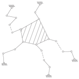
Figure 8. A pentagonal planar mechanism

In the planar case, it was shown in [SSB2, Proposition 2.4] that a necessary condition for a configuration ${\mathcal{V}}$ of such a linkage $\Gamma$ to be singular is that one of the following holds:

1. Two of its branch configurations  ${\mathcal{V}}^{({i_{1}})}$   and  ${\mathcal{V}}^{({i_{2}})}$   are aligned, with coinciding direction lines  $\operatorname{Line}(\mathbf{x}^{({i_{1}})}_{0},\mathbf{x}^{({i_{1}})}_{n^{({i_{1}})}})=\operatorname{Line}(\mathbf{x}^{({i_{2}})}_{0}\mathbf{x}^{({i_{2}})}_{n^{({i_{2}})}})$.

2. Three of its branch configurations are aligned, with direction lines in the same plane meeting in a single point $P$ (see Figure 9).

Figure 9. Singular configuration of type (b)

For simplicity we assume that  $k=3$,  so the two platforms are triangular.

5.2 Remark.

In the type (a) singularity there is obviously a sub-mechanism  $\Gamma^{\prime}$   which is isomorphic to an aligned closed chain, so the corresponding configuration  ${\mathcal{V}}\,^{\prime}$   is singular. Evidently, the caveat exemplified in §4.5 does not apply here, so in fact ${\mathcal{V}}$ is singular in  ${\mathcal{C}}_{\ast}(\Gamma)$.

5.3.

A sub-mechanism and its equivalent open chain. We shall now show that the same holds (generically) for type (b), using the approach of Section 3.

Consider the sub-mechanism  $\Gamma^{\prime}$   of $\Gamma$ obtained by omitting the third branch (but retaining the fixed platform), with base point at  $\mathbf{x}:=\mathbf{x}^{({3})}_{0}$   (the fixed endpoint of the omitted branch), and work point at  $\mathbf{y}:=\mathbf{x}^{({3})}_{n^{({3})}}$   (the moving endpoint of this branch). Let  ${\mathcal{V}}\,^{\prime}$   be the configuration of  $\Gamma^{\prime}$   corresponding to ${\mathcal{V}}$ of case (b) above (so in particular the remaining two branches are aligned).

Assume that the first branch has  $n:=n^{({1})}$   links, and the second has  $n^{\prime}:=n^{({2})}$   links. We may then choose “internal” parameters  $(\phi_{1},\dotsc,\phi_{n})$   for the first branch, and  $(\rho_{1},\dotsc,\rho_{n^{\prime}})$   for the second branch (as in the proof of Proposition 2.6). We can then express the lengths  $\ell=\|\mathbf{x}^{({1})}_{0}\mathbf{x}^{({1})}_{n}\|$   and  $m=\|\mathbf{x}^{({2})}_{0}\mathbf{x}^{({2})}_{n^{\prime}}\|$   as functions of  $(\phi_{1},\dotsc,\phi_{n})$   and  $(\rho_{1},\dotsc,\rho_{n^{\prime}})$,  respectively. Note that  $\Gamma^{\prime}$   has  $n+n^{\prime}+1$   degrees of freedom, so one additional parameter is needed. Two obvious choices are one of the “base angles”  $\phi=\angle(\mathbf{x}^{({1})}_{n}\mathbf{x}^{({1})}_{0}\mathbf{x}^{({2})}_{0})$   or  $\rho=\angle(\mathbf{x}^{({2})}_{n^{\prime}}\mathbf{x}^{({2})}_{0}\mathbf{x}^{({1})}_{0})$   for the two branches (see Figure 10).

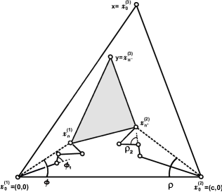
Figure 10. The sub-mechanism  $\Gamma^{\prime}$

However, for our purposes we shall need a different parameter, defined as follows:

Let $\mathbf{z}$ be the meeting point of the direction lines  $\operatorname{Line}(\mathbf{x}^{({1})}_{0}\mathbf{x}^{({1})}_{n})$   and  $\operatorname{Line}(\mathbf{x}^{({2})}_{0}\mathbf{x}^{({2})}_{n^{\prime}})$   for the two branches (this is the point $P$ of Figure 9). As our additional parameter we take the angle $\theta$ between the direction line  $\operatorname{Line}(\mathbf{x},\mathbf{y})$   for the (missing) third branch and the line  $\operatorname{Line}(\mathbf{y},\mathbf{z})$   (see Figure 11). Note that  $\theta=0$   or $\pi$ in our special configuration  ${\mathcal{V}}\,^{\prime}$.  Letting  $N:=n+n^{\prime}+1$,  the standard parametrization for the open $N$-chain  $\Gamma_{\operatorname{op}}^{N}$   defines a (local) diffeomorphism  $F:{\mathcal{C}}_{\ast}(\Gamma^{\prime})\to{\mathcal{C}}_{\ast}(\Gamma_{\operatorname{op}}^{N})$.

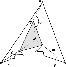
Figure 11. The parameters $\theta$, $m$, and $\ell$ for the sub-mechanism  $\Gamma^{\prime}$

In order to show that $F$ is a work-equivalent at  ${\mathcal{V}}\,^{\prime}$   to an aligned configuration  ${\mathcal{V}}^{({N})}$   of  $\Gamma_{\operatorname{op}}^{N}$   (Definition 2.2), we must show that  ${\mathcal{V}}\,^{\prime}$   is a generic singularity for  $\Gamma^{\prime}$    –  that is, that the reduced work map  $\tilde{\psi}:\widehat{{\mathcal{C}}}_{\ast}(\Gamma^{\prime})\to{\mathbb{R}}$   has an (isolated) singularity at  ${\mathcal{V}}\,^{\prime}$,  where $\tilde{\psi}$ assigns to any configuration ${\mathcal{V}}$ of  $\Gamma^{\prime}$   the length  $\tilde{\psi}({\mathcal{V}})=\|\mathbf{x},\mathbf{y}\|$.

It is difficult to write $\tilde{\psi}$ explicitly as a function of $\theta$: for this purpose it is simpler to use $\phi$ or $\rho$ as above. However, if we fix the lengths  $\ell=\ell(\phi_{1},\dotsc,\phi_{n})$   and  $m=m(\rho_{1},\dotsc,\rho_{n^{\prime}})$   of the direction vectors for the two branches, the resulting linkage  $\tilde{\Gamma}^{\prime}$   is a planar closed $4$-chain with one degree of freedom (parameterized by $\phi$, say), and the third vertex $\mathbf{y}$ of the moving triangle traces out a curve in  ${\mathbb{R}}^{2}$,  called the coupler curve for  $\tilde{\Gamma}^{\prime}$   (cf. [Hal, Ch. 4]). Therefore, the infinitesimal effect of a change in $\phi$ is the rotation of $\mathbf{y}$ about the point $\mathbf{z}$ described above (called the instantaneous point of rotation for  $\tilde{\Gamma}^{\prime}$).  In particular, the angle $\theta$ also changes, so we deduce that  $\operatorname{d}\!\theta/\operatorname{d}\!\phi\neq 0$   at the aligned configuration  ${\mathcal{V}}\,^{\prime}$.  This allows us to investigate the vanishing of  $\operatorname{d}\!\tilde{\psi}/\operatorname{d}\!\phi$   instead of  $\operatorname{d}\!\tilde{\psi}/\operatorname{d}\!\theta$.

This is the point where we are assuming genericity of  ${\mathcal{V}}\,^{\prime}$:  it might happen that the coupler curve is singular precisely at this point, in which case  $\operatorname{d}\!\theta/\operatorname{d}\!\phi$   may vanish, so we are no longer guaranteed that $\theta$ is a suitable local parameter. But such instances of case (b) are not generic.

Since in the reduced configuration space  $\widehat{{\mathcal{C}}}_{\ast}(\Gamma^{\prime})$   we do not allow rotation of  $\Gamma^{\prime}$   about the base-point  $\mathbf{x}_{\star}=(x_{0},y_{0})$,  we may assume that  $\mathbf{x}^{({1})}_{0}=(0,0)$   and  $\mathbf{x}^{({2})}_{0}=(c,0)$.  Write  $a:=\|\mathbf{x}^{({1})}_{n}\mathbf{x}^{({2})}_{n^{\prime}}\|$   and  $b:=\|\mathbf{x}^{({1})}_{n}\mathbf{y}\|$   for the (fixed) sides of the moving triangle (with fixed angle $\gamma$ between them), as in Figure 12.

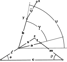
Figure 12. Angles and lengths in the sub-mechanism  $\Gamma^{\prime}$

We find that the following identities hold:

$$\begin{split}(\ell+s)\cos\phi~{}=&~{}c-(m+t)\cos\rho\\ (\ell+s)\sin\phi~{}=&~{}(m+t)\sin\rho\\ a\cos(\psi-\gamma)~{}=&~{}c-m\cos\rho-\ell\cos\phi\\ a\sin(\psi-\gamma)~{}=&~{}m\sin\rho-\ell\sin\phi\end{split}$$

(where $\psi$ is the angle between side $b$ and the $x$-axis), and:

$$\begin{split}a^{2}~{}=&~{}(c-m\cos\rho-\ell\cos\phi)^{2}+(m\sin\rho-\ell\sin\phi)^{2}\\ \tilde{\psi}^{2}~{}=&~{}(\ell\cos\phi+b\cos\psi-x_{0})^{2}+(\ell\sin\phi+b\sin\psi-y_{0})^{2}~{}.\end{split}$$

After differentiating we find:

$$\frac{\operatorname{d}(\cos\rho)}{\operatorname{d}\!\phi}~{}=~{}\frac{\ell t}{ms}\sin\rho\hskip 28.45274pt\text{and}\hskip 28.45274pt\frac{\operatorname{d}(\cos\psi)}{\operatorname{d}\!\phi}~{}=~{}-\frac{\ell}{s}\sin\psi~{},$$

and we deduce that  $\operatorname{d}\!\tilde{\psi}/\operatorname{d}\!\phi$   vanishes if and only if:

$$b\ell\sin(\phi-\psi)+bs\sin(\psi-\phi)+(s\cos\phi,s\sin\phi)\cdot(-y_{0},x_{0})+(b\cos\psi,b\sin\psi)\cdot(-y_{0},x_{0})=0.$$

This formula expresses the fact that the area of the triangle  $\triangle\mathbf{x}^{({1})}_{0}\mathbf{z}\mathbf{x}$   is the sum of the areas of the quadrangle  $\mathbf{x}^{({1})}_{0}\mathbf{x}^{({1})}_{n}\mathbf{y}\mathbf{x}$   and  $\triangle\mathbf{x}^{({1})}_{n}\mathbf{z}\mathbf{y}$,  which holds if and only if  $\mathbf{x}^{({1})}_{n}\mathbf{y}\mathbf{x}$   are aligned. From the formulas for  $\ell=\ell(\phi_{1},\dotsc,\phi_{n})$   and  $m=m(\rho_{1},\dotsc,\rho_{n^{\prime}})$   we see that  $\operatorname{d}\!\tilde{\psi}/\operatorname{d}\!\phi_{i}$   and  $\operatorname{d}\!\tilde{\psi}/\operatorname{d}\!\rho_{j}$   all vanish at  ${\mathcal{V}}\,^{\prime}$   (as for any aligned open chain), so in case (b)  $\nabla\tilde{\psi}=0$,  taken with respect to  $(\theta,\phi_{1},\dotsc,\phi_{n},\rho_{1},\dotsc,\rho_{n^{\prime}})$.  Since all but one of the parameters are the standard internal angles for open chains, we can check that the Morse indices for the reduced work maps of  $\Gamma^{\prime}$   and  $\Gamma_{\operatorname{op}}^{N}$   match up at  ${\mathcal{V}}\,^{\prime}$   and  $F({\mathcal{V}}\,^{\prime})$,  showing that $F$ is indeed a work-equivalence (see proof of Proposition 2.10). Thus we may apply Proposition 3.8 to deduce that  ${\mathcal{V}}\,^{\prime}$   is a cone singularity.

5.4 Summary.

Since the caveat of §4.5 does not apply to case (b), either (cf. §5.2), we have shown that for a generic triangular planar linkage $\Gamma$, any configuration  ${\mathcal{V}}\in{\mathcal{C}}_{\ast}(\Gamma)$   satisfying one of the necessary conditions (a) and (b) of [SSB2, Proposition 2.4] is ($S$-equivalent to) a generically non-transverse configuration (Definition 3.6). By Theorem 4.9 we can therefore deduce that it is indeed a topological singularity  –  that is, conditions (a) and (b) are also sufficient.

See [SSBB, Figure 8] for an illustration of such a cone singularity in a numerical example.

References

- [C] L. Caporaso, “Geometry of tropical moduli spaces and linkage of graphs”, preprint, 2010, arXiv:1001.2815.
- [CDR] R. Connelly, E.D. Demaine, & G. Rote, “Straightening polygonal arcs and convexifying polygonal cycles”, Discrete Comput. Geom. 30 (2003), pp. 205-239.
- [F] M.S. Farber, Invitation to Topological Robotics, European Mathematical Society, Zurich, 2008.
- [FTY] M.S. Farber, S. Tabachnikov, & S.A. Yuzvinskiĭ, “Topological robotics: motion planning in projective spaces”, Int. Math. Res. Notices 34 (2003), 1853-1870.
- [GA] C. Gosselin & J. Angeles, “Singularity analysis of Closed Loop Kinematic Chains”, IEEE Trans. on Robotics & Automation 6 (1990), pp. 281-290.
- [G] D.H. Gottlieb, “Topology and the robot arm”, Acta Applied Math. 11 (1988), pp. 117-121.
- [Hal] A.S. Hall, Jr., Kinematics and linkage design, Prentice-Hall, Englewood Cliffs, NJ, 1961.
- [Hau] J.-C. Hausmann, “Sur la topologie des bras articulés”, in S. Jackowski, R. Oliver, & K. Pawałowski, eds., Algebraic Topology - Poznán 1989, Lect. Notes Math. 1474, Springer Verlag, Berlin-New-York, 1991, pp. 146-159.
- [HK] J.-C. Hausmann & A. Knutson, “The cohomology ring of polygon spaces”, Ann. Inst. Fourier (Grenoble) 48 (1998), pp. 281-321.
- [Hi] M.W. Hirsch, Differential Topology, Springer-Verlag, Berlin-New York, 1976.
- [Ho] M. Holcomb, “On the Moduli Space of Multipolygonal Linkages in the Plane”, Topology & Applic. 154 (2007), pp. 124-143.
- [Hu] K.H. Hunt, Kinematic geometry of mechanisms, Oxford University Press, New York, 1978.
- [JS] D. Jordan & M. Steiner, “Compact surfaces as configuration spaces of mechanical linkages”, Israel J. Math. 122 (2001), pp. 175-187.
- [Ka] Y. Kamiyama, “The homology of the configuration space of a singular arachnoid mechanism”, JP J. Geom. Topol. 7 (2007), pp. 385–395.
- [KTe] Y. Kamiyama & M. Tezuka, “Symplectic volume of the moduli space of spatial polygons”, J. Math. Kyoto U. 39 (1999), pp. 557-575.
- [KTs] Y. Kamiyama & S. Tsukuda, “The configuration space of the -arms machine in the Euclidean space”, Topology & Applic. 154 (2007), pp. 1447-1464.
- [KM1] M. Kapovich & J. Millson, “On Moduli Space of Polygons in the Euclidean Plane”, J. Diff. Geom. 42 (1995), pp. 430-464.
- [KM2] M. Kapovich & J. Millson, “The symplectic geometry of polygons in Euclidean space”, J. Diff. Geom. 44 (1996), pp. 479-513.
- [KM3] M. Kapovich & J. Millson, “Universality theorems for configuration spaces of planar linkages”, Topology 41 (2002), pp. 1051-1107.
- [Ki] H.C. King, “Planar linkages and algebraic sets”, Turkish J. Math. 23 (1999), pp. 33-56.
- [L] J.M. Lee, Introduction to smooth manifolds, Springer-Verlag, Berlin-New York, 2003.
- [Ma] Y. Matsumoto, An Introduction to Morse Theory, American Math. Society, Providence, RI, 2002.
- [Me] J. P. Merlet, Parallel Robots, Kluwer Academic Publishers, Dordrecht, 2000.
- [MT] R. J. Milgram & J. C. Trinkle, ”The Geometry of Configuration Spaces for Closed Chains in Two and Three Dimensions”, Homology, Homotopy & Applic. 6 (2004), pp. 237-267.
- [OH] J. O’Hara, “The configuration space of planar spidery linkages”, Topology & Applic. 154 (2007), pp. 502-526.
- [Se] J.M. Selig, Geometric Fundamentals of Robotics, Springer-Verlag Mono. Comp. Sci., Berlin-New York, 2005.
- [Sh] I.R. Shafarevich, Basic algebraic geometry, 1. Varieties in projective space, Springer-Verlag, Berlin-New York, 1994.
- [SSBB] N. Shvalb, M. Shoham, H. Bamberger, & D. Blanc, “Topological and Kinematic Singularities for a Class of Parallel Mechanisms”, Math. Prob. in Eng. 2009 (2009), Art. 249349, pp. 1-12.
- [SSB1] N. Shvalb, M. Shoham, & D. Blanc, “The Configuration Space of Arachnoid Mechanisms”, Fund. Math. 17 (2005), pp. 1033-1042.
- [SSB2] N. Shvalb, M. Shoham and D. Blanc, “The configuration space of a parallel polygonal mechanism”, JP J. Geom. Top. 9 (2009), pp. 137-167.
- [T] L. W. Tsai, Robot Analysis - The mechanics of serial and parallel manipulators, Wiley interscience Publication - John Wiley & Sons, New York, 1999.
- [ZFB] D.S. Zlatanov, R.G. Felton, & B. Benhabib, “Singularity analysis of Mechanisms and Robots via a Motion–Space Model of the Instantaneous Kinematics”, Proceedings IEEE Conf. in Robotics & Automation (1994), pp. 980-985.
- [ZBG] D.S. Zlatanov, I.A. Bonev, & C.M. Gosselin, “Constraint Singularities as C-Space Singularities,”, 8th International Symposium on Advances in Robot Kinematics (ARK 2002), Caldes de Malavella, Spain, 2002.