Breaking Pseudo-Rotational Symmetry

Breaking Pseudo-Rotational Symmetry through $\boldsymbol{{\bf H}^{2}_{+}}$ Metric Deformation in the Eckart Potential Problem

Nehemias LEIJA-MARTINEZ ^†, David Edwin ALVAREZ-CASTILLO ^‡
and Mariana KIRCHBACH ^†

N. Leija-Martinez, D.E. Alvarez-Castillo and M. Kirchbach

^† Institute of Physics, Autonomous University of San Luis Potosi,
^† Av. Manuel Nava 6, San Luis Potosi, S.L.P. 78290, Mexico nemy@ifisica.uaslp.mx, mariana@ifisica.uaslp.mx

^‡ H. Niewodniczański Institute of Nuclear Physics, Radzikowskiego 152, 31-342 Kraków, Poland david.alvarez@ifj.edu.pl

Received October 12, 2011, in final form December 08, 2011; Published online December 11, 2011

The peculiarity of the Eckart potential problem on H${}^{2}_{+}$ (the upper sheet of the two-sheeted two-dimensional hyperboloid), to preserve the $(2l+1)$-fold degeneracy of the states typical for the geodesic motion there, is usually explained in casting the respective Hamiltonian in terms of the Casimir invariant of an so(2,1) algebra, referred to as potential algebra. In general, there are many possible similarity transformations of the symmetry algebras of the free motions on curved surfaces towards potential algebras, which are not all necessarily unitary. In the literature, a transformation of the symmetry algebra of the geodesic motion on H${}_{+}^{2}$ towards the potential algebra of Eckart’s Hamiltonian has been constructed for the prime purpose to prove that the Eckart interaction belongs to the class of Natanzon potentials. We here take a different path and search for a transformation which connects the $(2l+1)$ dimensional representation space of the pseudo-rotational so(2,1) algebra, spanned by the rank-$l$ pseudo-spherical harmonics, to the representation space of equal dimension of the potential algebra and find a transformation of the scaling type. Our case is that in so doing one is producing a deformed isometry copy to ${\mathbf{H}}^{2}_{+}$ such that the free motion on the copy is equivalent to a motion on ${\mathbf{H}}^{2}_{+}$, perturbed by a $\coth$ interaction. In this way, we link the so(2,1) potential algebra concept of the Eckart Hamiltonian to a subtle type of pseudo-rotational symmetry breaking through ${\mathbf{H}}^{2}_{+}$ metric deformation. From a technical point of view, the results reported here are obtained by virtue of certain nonlinear finite expansions of Jacobi polynomials into pseudo-spherical harmonics. In due places, the pseudo-rotational case is paralleled by its so(3) compact analogue, the cotangent perturbed motion on S². We expect awareness of different so(2,1)/so(3) isometry copies to benefit simulation studies on curved manifolds of many-body systems.

pseudo-rotational symmetry; Eckart potential; symmetry breaking through metric deformation

47E05; 81R40

1 Introduction

Group theoretical approaches to bound state problems in physics have played a pivotal róle in our understanding of spectra classifications. It is a well known fact, that several of the exactly solvable quantum mechanical potentials give rise to spectra which fall into the irreducible representations of certain Lie groups. As a representative case, we wish to mention the widely studied class of Natanzon potentials [2] known to produce spectra that populate multiplets of the pseudo-rotational algebras so(2,2)/so(2,1). This phenomenon has been well understood in casting the Hamiltonians of the potentials under consideration as Casimir invariants of so(2,2)/so(2,1) algebras in representations not necessarily unitarily equivalent to the pseudo-rotational and referred to as “potential algebras” [3, 4]. One popular representative of the Natanzon class potentials is the Eckart potential, suggested by Manning and Rosen [5] for the description of the vibrational modes of diatomic molecules. Its so(2,2)/so(2,1) potential algebras have been constructed, among others, in [6, 7, 8, 9, 10, 11]. One can start with considering the Eckart potential on H², the two-sheeted 2D hyperbolic surface, defined as

$${\mathbf{H}}^{2}_{\pm}:\ z^{2}-x^{2}-y^{2}=R^{2},$$

where $R$ is a constant. This geometry has been studied in great detail [12], and finds applications, among others, as a coherent state manifold [13, 14]. One usually chooses the upper sheet ${\mathbf{H}}^{2}_{+}$, which corresponds to the following parametrization in global coordinates

$$z=R\cosh\eta,\qquad x=R\sinh\eta\cos\varphi,$$

$$y=R\sinh\eta\sin\varphi,\qquad z>\sqrt{x^{2}+y^{2}},\qquad\eta\in[0,\infty).$$

The free geodesic motion on ${\mathbf{H}}^{2}_{+}$ is now determined by the eigenvalue problem of the squared pseudo-angular momentum operator ${\mathcal{C}}$

$${\mathcal{H}}{\mathcal{Y}}_{l}^{m}(\eta,\varphi)=-\frac{\hbar^{2}}{2M}l(l+1){\mathcal{Y}}_{l}^{m}(\eta,\varphi),\qquad{\mathcal{H}}=-\frac{\hbar^{2}}{2M}{\mathcal{C}},$$

$${\mathcal{C}}=\frac{1}{\sinh\eta}\frac{\partial}{\partial\eta}\sinh\eta\frac{\partial}{\partial\eta}+\frac{1}{\sinh^{2}\eta}\frac{\partial^{2}}{\partial\varphi^{2}},$$ (1)

so that the symmetry of the Hamiltonian, ${\mathcal{H}}$, is so(2,1). Here, ${\mathcal{Y}}_{l}^{m}(\eta,\varphi)$ are the standard pseudo-spherical harmonics [15]

$${\mathcal{Y}}_{l}^{m}(\eta,\varphi)=P_{l}^{m}(\cosh\eta)e^{im\varphi},\qquad\eta\in(-\infty,+\infty),$$ (2)

with $P_{l}^{m}(\cosh\eta)$ being the associated Legendre functions of a hyperbolic cosines argument. In [10] it has been shown that the following particular similarity transformation of ${\mathcal{C}}$

$${\mathbf{F}}(\eta){\mathcal{C}}{\mathbf{F}}^{-1}(\eta)=\widetilde{\mathcal{C}},\qquad{\mathbf{F}}(\eta)=\sqrt{\frac{\sinh 2g(r)}{g^{\prime}(r)}},\qquad\tanh^{2}g(r)=z=e^{-r},$$ (3)

transforms equation (1) into a Natanzon equation in the $z$ variable, and to the central Eckart potential problem in ordinary 3D flat position space in the $r$ variable. In this fashion it became possible to cast the Schrödinger Hamilton operator with the Eckart potential, treated as a central interaction, in the form of a particular Casimir invariant of the so(2,1) algebra.

Compared to [6], and [10], we here exclusively focus on the relationship between the free, and the $\coth\eta$ perturbed motions on H${}_{+}^{2}$ and find a transformation that connects the $({\mathcal{C}}+2b\coth\eta)$- and ${\mathcal{C}}$-eigenvalue problems and their respective invariant spaces, a transformation which has not been reported in the literature so far. The ${\mathcal{C}}$ invariant spaces are $(2l+1)$-dimensional, non-unitary, and spanned by the pseudo-spherical harmonics in (2). Towards our goal, we develop a technique for solving the $\left({\mathcal{C}}+2b\coth\eta\right)$-eigenvalue problem which slightly differs from the one of standard use. Ordinarily, the respective 1D Schrödinger equation is resolved by reducing it to the hyper-geometric differential equation satisfied by the Jacobi polynomials. We here instead construct the solutions directly in the basis of the free geodesic motion, i.e. in the ${\mathcal{Y}}_{l}^{m}(\eta,\varphi)$ basis. In so doing, we find superpositions of exponentially damped pseudo-spherical harmonics which describe the perturbance by a hyperbolic cotangent function of the free geodesic motion on H${}_{+}^{2}$. The matrix similarity transformation between the ${\mathcal{C}}$ and $({\mathcal{C}}+2b\coth\eta)$ eigenvalue problems is then read off from those decompositions which allow to interpret the Hamiltonian of the perturbed motion as a Casimir invariant of an so(2,1) algebra in a representation unitarily nonequivalent to the pseudo-rotational. The consequence is a breakdown of the pseudo-rotational invariance of the free geodesic motion only at the level of the representation functions which becomes apparent through a deformation of the metric of the hyperbolic space, and without a breakdown of the $(2l+1)$-fold degeneracy patterns in the spectrum. Moreover, due to cancellation effects occurring by virtue of specific recurrence relations among associated Legendre functions, the similarity transformation presents itself simple and, as explained in the concluding summary section, may specifically benefit applications in problems with an approximate so(2,1) symmetry. The problem under investigation is well known to transform into the Rosen–Morse potential problem on S² by a complexification of the hyperbolic angle, followed by a complexification of the strength of the $\coth\eta$ potential. On this basis, the statement on the symmetry and degeneracy properties of the Eckart potential on H${}_{+}^{2}$ can easily be transferred to the trigonometric Rosen–Morse potential problem on S².

The paper is structured as follows. In the next section we present the eigenvalue problem of the $\coth$-perturbed particle motion on H${}_{+}^{2}$. There, we furthermore work out the respective solutions as expansions in the basis of the standard pseudo-spherical harmonics, find the non-unitary transformation relating the free and the perturbed geodesic motions, present the class of recurrence relations among associated Legendre functions that triggers the above similarity transformation. In due places, the conclusions regarding the Rosen–Morse potential problem on S² have been drawn in parallel to those regarding the Eckart potential. The paper ends with concise summary and conclusions.

2 Scalar particle motions on $\boldsymbol{{\bf H}^{2}_{+}}$ and $\boldsymbol{{\rm S}^{2}}$ and representations
for the so(2,1) and so(3) algebras unitarily nonequivalent
to the respective pseudo-rotational and rotational ones

2.1 From free to perturbed motions

We begin with taking a closer look on equation (1) for the particular case of $l=0$

$$-\frac{\hbar^{2}}{2M}{\mathcal{C}}{\mathcal{Y}}_{0}^{0}(\eta,\varphi)=0,$$ (4)

and subject it to a similarity transformation to obtain

$$-\frac{\hbar^{2}}{2M}\left[{\mathbf{F}}^{-1}(\eta){\mathcal{C}}{\mathbf{F}}(\eta)\right]\left[{\mathbf{F}}^{-1}(\eta){\mathcal{Y}}_{0}^{0}(\eta,\varphi)\right]=-\frac{\hbar^{2}}{2M}{\widetilde{\mathcal{C}}}\left[{\mathbf{F}}^{-1}(\eta){\mathcal{Y}}_{0}^{0}(\eta,\varphi)\right]=0,$$ (5)

with $\widetilde{\mathcal{C}}={\mathbf{F}}^{-1}(\eta){\mathcal{C}}{\mathbf{F}}(\eta)$. The general expression for any transformation in (5) is easily worked out (cf. [10]) and reads

$$\widetilde{\mathcal{C}}={\mathbf{F}}^{-1}(\eta){\mathcal{C}}{\mathbf{F}}(\eta)={\mathcal{C}}+\frac{1}{{\mathbf{F}}(\eta)}\frac{{\mathrm{d}}^{2}{\mathbf{F}}(\eta)}{{\mathrm{d}}^{2}\eta}+2\frac{1}{{\mathbf{F}}(\eta)}\frac{{\mathrm{d}}{\mathbf{F}}(\eta)}{{\mathrm{d}}\eta}\left(\frac{{\mathrm{d}}}{{\mathrm{d}}\eta}+\frac{1}{2}\coth\eta\right).$$

We here chose ${\mathbf{F}}(\eta)$ differently than in (3) and consider the following scaling similarity transformation

$${\mathbf{F}}(\eta)=e^{\frac{\alpha_{(l=0)}\eta}{2}},\qquad\alpha_{(l=0)}=4b.$$ (6)

Substitution of (6) into (5) amounts to

$$-\frac{\hbar^{2}}{2M}{\widetilde{C}}{\widetilde{\mathcal{Y}}}_{0}^{0}(\eta,\varphi)=-\frac{\hbar^{2}}{2M}\left[e^{-\frac{\alpha_{(l=0)}\eta}{2}}{\mathcal{C}}e^{\frac{\alpha_{(l=0)}\eta}{2}}\right]\,\left[e^{-\frac{\alpha_{(l=0)}\eta}{2}}{\mathcal{Y}}_{0}^{0}(\eta,\varphi)\right]$$

$$\phantom{-\frac{\hbar^{2}}{2M}{\widetilde{C}}{\widetilde{\mathcal{Y}}}_{0}^{0}(\eta,\varphi)}{}=-\frac{\hbar^{2}}{2M}\left({\mathcal{C}}-\frac{\alpha_{(l=0)}^{2}}{4}+2b\coth\eta\right){\widetilde{\mathcal{Y}}_{0}^{0}}(\eta,\varphi)=0,$$

$${\widetilde{\mathcal{Y}}_{0}^{0}}(\eta,\varphi)=e^{-\frac{\alpha_{(l=0)}\eta}{2}}{\mathcal{Y}}_{0}^{0}(\eta,\varphi),$$ (7)

which turns equivalent to the standard form of the $\coth\eta$ perturbed motion on H${}_{+}^{2}$, for the ground state

$$-\frac{\hbar^{2}}{2M}\left({\mathcal{C}}+2b\coth\eta\right){\widetilde{\mathcal{Y}}_{0}^{0}}(\eta,\varphi)=-\frac{\hbar^{2}}{2M}4b^{2}{\widetilde{\mathcal{Y}}_{0}^{0}}(\eta,\varphi),$$ (8)

where the special notation, ${\widetilde{\mathcal{Y}}_{0}^{0}}(\eta,\varphi)$, has been introduced in (7) for the exponentially damped pseudo-spherical harmonic under consideration. We now notice that ${\mathcal{C}}$ in (4) is the Casimir invariant of the so(1,2) isometry algebra of the ${\mathbf{H}}^{2}$ hyperboloid, described by the $|{\mathcal{Y}}_{0}^{0}(\eta,\varphi)|$ unit surface, displayed in the l.h.s. of Fig. 1, and that, correspondingly, ${\widetilde{\mathcal{C}}}=e^{-\frac{\alpha_{(l=0)}\eta}{2}}{\mathcal{C}}e^{\frac{\alpha_{(l=0)}\eta}{2}}$ in (7) is same on the deformed surface $e^{-\alpha_{(l=0)}\eta/2}|{\mathcal{Y}}_{0}^{0}(\eta,\varphi)|$, shown on the r.h.s. in Fig. 1.

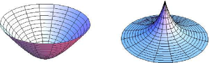
Figure 1: Breaking of the pseudo-rotational symmetry at the level of the metric. A regular H${}_{+}^{2}$ hyperboloid associated with the so(1,2) scalar, $(z^{2}-x^{2}-y^{2})$ (left), and its non-unitary deformation, $\exp(-\alpha_{(l=0)}\eta/2)(z^{2}-x^{2}-y^{2})$ (right) with $\alpha_{(l=0)}=4b$, and $\eta=\coth^{-1}\frac{z}{\sqrt{x^{2}+y^{2}}}$. Schematic presentation for $b=1$.

From this perspective, equation (7) shows that the free motion on the deformed metric in Fig. 1 is equivalent to the $\coth\eta$ perturbed motion on ${\mathbf{H}}^{2}_{+}$. The rest of the article is devoted to generalize equation (7) to higher $l$ values. From now onwards we shall switch to dimensionless units, $\hbar=1$, $2M=1$, for the sake of simplicity.

In parallel, we notice that as long as so(1,2), and so(3) are related by a Wigner rotation, ${\mathcal{C}}$ in equation (1) is related to the well known expression of the standard squared orbital angular momentum ${\mathbf{L}}^{2}$

$${\mathbf{L}}^{2}=-\frac{1}{\sin\theta}\frac{\partial}{\partial\theta}\sin\theta\frac{\partial}{\partial\theta}-\frac{1}{\sin^{2}\theta}\frac{\partial^{2}}{\partial\varphi^{2}},$$

by a complexification of the polar angle

$${\mathbf{L}}^{2}\stackrel{{\scriptstyle\theta\to i\eta}}{{\longrightarrow}}{\mathcal{C}}.$$

It is the type of complexification that takes the hyperboloid H${}^{2}_{+}$ to the sphere S². Correspondingly, the scaling transformation in equation (6) will take the free geodesic motion on S² to the one perturbed by the trigonometric Rosen–Morse potential there

$${\widetilde{\mathbf{L}}^{2}}\widetilde{Y}_{0}^{0}(\theta,\varphi)=\left({\mathbf{L}}^{2}-2b\cot\theta-\frac{\alpha_{(l=0)}^{2}}{4}\right)\widetilde{Y}_{0}^{0}(\theta,\varphi)=0,$$

$$\widetilde{Y}_{0}^{0}(\theta,\varphi)=e^{-\frac{\alpha_{(l=0)}\theta}{2}}Y_{0}^{0}(\theta,\varphi).$$ (9)

The counterpart of Fig. 1 is displayed on Fig. 2.

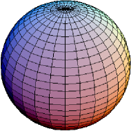
Figure 2: The S² spherical metric, $|Y_{00}(\theta,\varphi)|$ (left) in comparison to the exponentially deformed one, $|\widetilde{Y}_{00}(\theta,\varphi)|$ (right) for b=1. The cotangent perturbed rigid rotor on S² is equivalent (up to a shift by constant) to free motion on the deformed metric, as visible from equation (9).

2.2 The perturbed geodesic motions

We now consider the general case of a perturbance of the free geodesic motion in (1) by a hyperbolic cotangent potential

$$\left[{\mathcal{C}}+2b\coth\eta\right]{\mathcal{X}}(\eta,\varphi)$$

$$\qquad{}=\left[\frac{1}{\sinh\eta}\frac{\partial}{\partial\eta}\sinh\eta\frac{\partial}{\partial\eta}+\frac{1}{\sinh^{2}\eta}\frac{\partial^{2}}{\partial\varphi^{2}}+2b\coth\eta\right]{\mathcal{X}}(\eta,\varphi)=-\epsilon{\mathcal{X}}(\eta,\varphi),$$ (10)

$${\mathcal{X}}(\eta,\varphi)=e^{-\frac{\alpha\eta}{2}}F(\eta)e^{i{\widetilde{m}}\varphi},$$ (11)

where $\epsilon$ stands for the energy in dimensionless units. The $\eta$ and $\varphi$ dependencies of the eigenfunctions separate, and we admitted for the possibility that ${\widetilde{m}}$ may not take same value as the magnetic quantum number in the free case. In what follows we attach indices to ${\mathcal{X}}(\eta,\varphi)$ as ${\mathcal{X}}(\eta,\varphi)\longrightarrow{\mathcal{X}}_{l}^{\widetilde{m}}(\eta,\varphi)$, and search for $({\mathcal{C}}+2b\coth\eta)$ eigenfunctions in the form of superpositions of damped pseudo-spherical harmonics, ${\widetilde{\mathcal{Y}}}_{l}^{m}(\eta,\varphi)$, with $m\in[{\widetilde{m}},l]$, according to

$${\mathcal{X}}_{l}^{\widetilde{m}}(\eta,\varphi)=\left[\sum_{m={\widetilde{m}}}^{m=l}a_{({\widetilde{m}}+1)(m+1)}^{l}e^{-im\varphi}{\widetilde{\mathcal{Y}}}_{l}^{m}(\eta,\varphi)\right]e^{i{\widetilde{m}}\varphi},$$

$${\widetilde{\mathcal{Y}}}_{l}^{m}(\eta,\varphi)=e^{-\frac{\alpha\eta}{2}}{\mathcal{Y}}_{l}^{m}(\eta,\varphi).$$ (12)

Furthermore, $a_{({\widetilde{m}}+1)(m+1)}^{l}e^{i({\widetilde{m}}-m)\varphi}$ (with constant $a_{({\widetilde{m}}+1)(m+1)}^{l}$) are elements of an $(l+1)\times(l+1)$ dimensional matrix. We begin with the observation that upon substituting (12) in (10), the particle motion on H${}_{+}^{2}$, hindered by a $\coth\eta$ interaction, equivalently rewrites to

$$e^{-\frac{\alpha\eta}{2}}\left[\frac{1}{\sinh\eta}\frac{\partial}{\partial\eta}\sinh\eta\frac{\partial}{\partial\eta}-\frac{{\widetilde{m}}^{2}}{\sinh^{2}\eta}+\frac{\alpha^{2}}{4}+\alpha D\right]\left[\sum_{|m|=|{\widetilde{m}}|}^{l}a^{l}_{(|{\widetilde{m}}|+1)(|m|+1)}P_{l}^{|m|}(\cosh\eta)\right]e^{i{\widetilde{m}}\varphi}$$

$$=-\epsilon e^{-\frac{\alpha\eta}{2}}\left[\sum_{|m|=|{\widetilde{m}}|}^{l}a^{l}_{(|{\widetilde{m}}|+1)(|m|+1)}P_{l}^{|m|}(\cosh\eta)\right]e^{i{\widetilde{m}}\varphi},\quad D=\left(\frac{2b}{\alpha}-\frac{1}{2}\right)\coth\eta-\frac{\partial}{\partial\eta},$$ (13)

where we dragged the exponential function through ${\mathcal{C}}$ from the very right to the very left, and inserted equation (12) for ${\mathcal{X}}_{l}^{\widetilde{m}}(\eta,\varphi)$. Next we consider the particular case when the sum in equation (12) contains one term only, i.e. when ${\widetilde{m}}=l$:

$${\mathcal{X}}_{l}^{l}(\eta,\varphi)=a^{l}_{(l+1),(l+1)}e^{-\frac{\alpha\eta}{2}}P_{l}^{l}(\cosh\eta)e^{il\varphi}.$$

In this case, the part of (13) behind the exponential would reduce to the differential equation for the associated Legendre functions, shifted by the constant, $\alpha^{2}/4$, provided

$$DP_{l}^{l}(\cosh\eta)=0,\qquad P_{l}^{l}(\cosh\eta)=\sinh^{l}\eta,$$ (14)

were to hold valid. The latter equation imposes the following condition on $\alpha$

$$\alpha\longrightarrow\alpha_{l},\qquad\alpha_{l}=\frac{2b}{l+\frac{1}{2}},$$ (15)

where we re-labeled $\alpha$ to $\alpha\to\alpha_{l}$. In effect, the $({\mathcal{C}}+2b\coth\eta)$ eigenvalue problem simplifies to the ${\mathcal{C}}$ eigenvalue problem subjected to a scaling similarity transformation according to

$$\left[{\mathcal{C}}+2b\coth\eta\right]{\mathcal{X}}_{l}^{l}(\eta,\varphi)=\left[e^{-\frac{\alpha_{l}\eta}{2}}\left({\mathcal{C}}+\frac{\alpha_{l}^{2}}{4}\right)e^{\frac{\alpha_{l}\eta}{2}}\right]{\mathcal{X}}_{l}^{l}(\eta,\varphi)=\left(l(l+1)+\frac{\alpha_{l}^{2}}{4}\right){\mathcal{X}}_{l}^{l}(\eta,\varphi),$$

$${\mathcal{X}}_{l}^{l}(\eta,\varphi)=a^{l}_{(l+1),(l+1)}e^{-\frac{\alpha_{l}\eta}{2}}{\mathcal{Y}}_{l}^{l}(\eta,\varphi).$$ (16)

We set $a^{l}_{(l+1),(l+1)}=1$ for simplicity. As a next step, we consider the case of a two-term decomposition in (12), when

$${\mathcal{X}}_{l}^{l-1}(\eta,\varphi)=e^{-\frac{\alpha_{l}\eta}{2}}\left(a^{l}_{ll}P_{l}^{l-1}(\cosh\eta)+a^{l}_{(l)(l+1)}P_{l}^{l}(\cosh\eta)\right)e^{i(l-1)\varphi}.$$

Substituting in (10), and dragging the exponential factor again from the very right to the very left, amounts to

$$\left[{\mathcal{C}}+2b\coth\eta\right]{\mathcal{X}}_{l}^{l-1}(\eta,\varphi)=e^{-\frac{\alpha_{l}\eta}{2}}\left[\frac{1}{\sinh\eta}\frac{\partial}{\partial\eta}\sinh\eta\frac{\partial}{\partial\eta}-\frac{(l-1)^{2}}{\sinh^{2}\eta}+\frac{\alpha^{2}_{l}}{4}+\alpha_{l}D_{l}\right]$$

$$\qquad\quad{}\times\Big{(}a^{l}_{ll}P_{l}^{l-1}(\cosh\eta)+a^{l}_{(l)(l+1)}P_{l}^{l}(\cosh\eta)\Big{)}e^{i(l-1)\varphi}$$

$$\qquad{}=\left(l(l+1)+\frac{\alpha_{l}^{2}}{4}\right)\!e^{-\frac{\alpha\eta}{2}}\Big{(}a^{l}_{ll}P_{l}^{l-1}(\cosh\eta)+a^{l}_{(l)(l+1)}P_{l}^{l}(\cosh\eta)\Big{)}e^{i(l-1)\varphi}\!,$$

$$D_{l}=\left(l\coth\eta-\frac{\partial}{\partial\eta}\right),$$ (17)

where the expression for $D_{l}$, corresponding to $D$ from (13) with an attached label $\ell$, i.e. $D\to D_{l}$, has been obtained in making use use of (15). The unknown constant, $a^{l}_{(l)(l+1)}$, is now determined from the condition

$$-\frac{(l-1)^{2}}{\sinh^{2}\eta}a_{(l)(l+1)}^{l}P_{l}^{l}(\cosh\eta)+\alpha_{l}D_{l}a_{ll}^{l}P_{l}^{l-1}(\cosh\eta)=-\frac{l^{2}}{\sinh^{2}\eta}a_{(l)(l+1)}^{l}P_{l}^{l}(\cosh\eta),$$

setting once again $a^{l}_{ll}=1$. Taking into account that $P_{l}^{l-1}(\cosh\eta)=\sinh^{l-1}\eta\cosh\eta$, one arrives at the constraint

$$a^{l}_{(l)(l+1)}=\frac{\alpha_{l}}{-l^{2}+(l-1)^{2}},$$

thus fixing the $a^{l}_{l(l+1)}$ value. In consequence, the eigenvalue problem in equation (17) simplifies to same form as previously found in equation (16), namely

$$\left[{\mathcal{C}}+2b\coth\eta\right]{\mathcal{X}}_{l}^{l-1}(\eta,\varphi)=\left[e^{-\frac{\alpha_{l}\eta}{2}}\left({\mathcal{C}}+\frac{\alpha_{l}^{2}}{4}\right)e^{\frac{\alpha_{l}\eta}{2}}\right]{\mathcal{X}}_{l}^{l-1}(\eta,\varphi)$$

$$\hphantom{\left[{\mathcal{C}}+2b\coth\eta\right]{\mathcal{X}}_{l}^{l-1}(\eta,\varphi)}{}=\left[\widetilde{\mathcal{C}}+\frac{\alpha^{2}_{(l)}}{4}\right]{\mathcal{X}}_{l}^{l-1}(\eta,\varphi)=\left(l(l+1)+\frac{\alpha_{(l)}^{2}}{4}\right){\mathcal{X}}_{l}^{l-1}(\eta,\varphi).$$

Proceeding successively in this way, the coefficients $a^{l}_{({\widetilde{m}}+1)(m+1)}$ can be found imposing the following condition

$$\left[-\frac{{\widetilde{m}}^{2}}{\sinh^{2}\eta}+\alpha_{l}D_{l}\right]\left[\sum_{m={\widetilde{m}}}^{m=l}a_{({\widetilde{m}}+1)(m+1)}^{l}e^{-im\varphi}{\mathcal{Y}}_{l}^{m}(\eta,\varphi)\right]$$

$$\qquad{}=-\left[\sum_{m={\widetilde{m}}}^{m=l}a_{({\widetilde{m}}+1)(m+1)}^{l}e^{-im\varphi}\frac{m^{2}}{\sinh^{2}\eta}{\mathcal{Y}}_{l}^{m}(\eta,\varphi)\right],$$ (18)

guaranteed by virtue of recurrence relations among associated Legendre functions of the type

$$D_{(l=1)}P_{1}^{0}(\cosh\eta)=\frac{1^{2}}{\sinh^{2}\eta}P_{1}^{1}(\cosh\eta),$$ (19)

$$D_{(l=2)}P_{2}^{1}(\cosh\eta)=\frac{1}{\sinh^{2}\eta}P_{2}^{2}(\cosh\eta),$$ (20)

$$D_{(l=2)}P_{2}^{0}(\cosh\eta)=\frac{2}{3}\frac{1}{\sinh^{2}\eta}P_{2}^{1}(\cosh\eta),\quad\mbox{etc.}$$ (21)

In combination with the identity, $P_{l}^{|m|}(\cosh\eta)=e^{-im\varphi}{\mathcal{Y}}_{l}^{m}(\eta,\varphi)$, equations (18)–(21) allow to cast the general $({\mathcal{C}}+2b\coth\eta)){\mathcal{X}}_{l}^{{\widetilde{m}}}(\eta,\varphi)$ eigenvalue problem for any $l$ and ${\widetilde{m}}$ into the following equivalent form

$$\left[{\mathcal{C}}+2b\coth\eta\right]{\mathcal{X}}_{l}^{{\widetilde{m}}}(\eta,\varphi)=\left[\widetilde{{\mathcal{C}}}+\frac{\alpha_{l}^{2}}{4}\right]{\mathcal{X}}_{l}^{{\widetilde{m}}}(\eta,\varphi)=\left(l(l+1)+\frac{\alpha_{l}^{2}}{4}\right){\mathcal{X}}_{l}^{{\widetilde{m}}}(\eta,\varphi),$$ (22)

with ${\mathcal{X}}_{l}^{{\widetilde{m}}}(\eta,\varphi)$ standing for the exact solutions of the Eckart potential on H${}_{+}^{2}$ obtained from the ansatz in (12). Omitting normalization factors for simplicity, the eigenfunctions to (22) for some of the lowest $l$ values, now cast in matrix form, are calculated as

$$\begin{pmatrix}{\mathcal{X}}_{1}^{0}(\eta,\varphi)\\ {\mathcal{X}}_{1}^{1}(\eta,\varphi)\end{pmatrix}=e^{-\frac{2b\eta}{3}}\begin{pmatrix}1&-\frac{4b}{3}e^{-i\varphi}\\ 0&1\end{pmatrix}\begin{pmatrix}{\mathcal{Y}}_{1}^{0}(\eta,\varphi)\\ {\mathcal{Y}}_{1}^{1}(\eta,\varphi)\end{pmatrix},$$ (23)

$$\begin{pmatrix}{\mathcal{X}}_{2}^{0}(\eta,\varphi)\\ {\mathcal{X}}_{2}^{1}(\eta,\varphi)\\ {\mathcal{X}}_{2}^{2}(\eta,\varphi)\end{pmatrix}=e^{-\frac{2b\eta}{5}}\begin{pmatrix}1&-\frac{8b}{15}e^{-i\varphi}&\frac{8b^{2}}{75}e^{-2i\varphi}\\ 0&1&-\frac{4b}{15}e^{-i\varphi}\\ 0&0&1\end{pmatrix}\begin{pmatrix}{\mathcal{Y}}_{2}^{0}(\eta,\varphi)\\ {\mathcal{Y}}_{2}^{1}(\eta,\varphi)\\ {\mathcal{Y}}_{2}^{2}(\eta,\varphi)\end{pmatrix}.$$ (24)

Admittedly, the above expressions are easier obtained parting from the (unnormalized) solutions of equation (10) known from the literature [16] to be expressed in terms of Jacobi polynomials, here denoted by ${\mathcal{P}}_{n}^{\gamma,\delta}$, as

$${\mathcal{X}}_{l}^{\widetilde{m}}(\eta,\varphi)=\sinh^{l}\eta e^{-\frac{\alpha_{l}\eta}{2}}{\mathcal{P}}_{n}^{\gamma_{l},\delta_{l}}(\coth\eta)e^{i{\widetilde{m}}\varphi},$$

$$\gamma_{l}=\frac{b}{l+\frac{1}{2}}-\left(l+\frac{1}{2}\right),\qquad\delta_{l}=-\frac{b}{l+\frac{1}{2}}-\left(l+\frac{1}{2}\right),\qquad l={\widetilde{m}}+n.$$ (25)

Comparison of (25) to (12) allows to conclude on the existence of finite nonlinear decompositions of the Jacobi polynomials into associated Legendre functions $(P_{l}^{m})$ according to

$$\sinh^{l}\eta{\mathcal{P}}_{n}^{\gamma_{l},\delta_{l}}(\coth\eta)=\sum_{m={\widetilde{m}}}^{m=l}a_{({\widetilde{m}}+1)(m+1)}^{l}P_{l}^{m}(\cosh\eta).$$

The latter equation can equally well be used to pin down the expansion coefficients upon using the orthogonality properties of the associated Legendre functions.

The $({\mathcal{C}}+2b\coth\eta)$ eigenvalue problem is closely related to the rigid rotator problem on S² perturbed by a cotangent interaction, $({\mathbf{L}}^{2}-2b\cot\theta)$. The two problems have several features in common. Also the $\cot\theta$ interaction preserves the $(2l+1)$-fold degeneracy patterns characterizing the spectrum of the free geodesic motion, despite its non-commutativity with ${\mathbf{L}}^{2}$. The similarities between these two cases are due to their interrelation by the following complexifications

$${\mathcal{C}}+2b\coth\eta\stackrel{{\scriptstyle\eta\to i\theta,b\to-ib}}{{\longrightarrow}}{\mathbf{L}}^{2}-2b\cot\theta.$$ (26)

It is straightforward to prove that in effect of the complexifications in (26), the equation (22) is transformed to

$$\left[{\mathbf{L}}^{2}-2b\cot\theta\right]{\mathcal{X}}_{l}^{\widetilde{m}}(\theta,\varphi)=\left[e^{-\frac{\alpha_{l}\eta}{2}}\left({\mathbf{L}}^{2}-\frac{\alpha_{l}^{2}}{4}\right)e^{\frac{\alpha_{l}\eta}{2}}\right]{\mathcal{X}}_{l}^{\widetilde{m}}(\theta,\varphi)$$

$$\hphantom{\left[{\mathbf{L}}^{2}-2b\cot\theta\right]{\mathcal{X}}_{l}^{\widetilde{m}}(\theta,\varphi)=}{}=\left(\widetilde{\mathbf{L}}^{2}-\frac{\alpha_{l}^{2}}{4}\right){\mathcal{X}}_{l}^{\widetilde{m}}(\theta,\varphi)=\left(l(l+1)-\frac{\alpha_{(l)}^{2}}{4}\right){\mathcal{X}}_{l}^{\widetilde{m}}(\theta,\varphi),$$ (27)

with ${\mathcal{X}}_{l}^{\widetilde{m}}(\theta,\varphi)$ being given as

$${\mathcal{X}}_{l}^{\widetilde{m}}(\theta,\varphi)=\left[\sum_{m={\widetilde{m}}}^{m=l}c_{l}a_{({\widetilde{m}}+1)(m+1)}^{l}e^{-im\varphi}{\widetilde{Y}}_{l}^{m}(\theta,\varphi)\right]e^{i{\widetilde{m}}\varphi},$$

$${\widetilde{Y}}_{l}^{m}(\theta,\varphi)=e^{-\frac{\alpha_{l}\theta}{2}}Y_{l}^{m}(\theta,\varphi),$$ (28)

where $Y_{l}^{m}(\theta,\varphi)$ are the standard spherical harmonics, and the constants $|c_{l}|=1$ account for possible sign changes in $a_{({\widetilde{m}}+1)(m+1)}^{l}$ in depending on the power of $(ib)$ contained there. In conclusion, also the cotangent perturbed rigid rotator can be cast into the form of a Casimir invariant of the so(3) algebra though in a representation unitarily nonequivalent to the rotational.

Also for the latter case the exact solutions of equation (27) are known [17], and expressed in terms of real Romanovski polynomials [18] as

$${\mathcal{X}}_{l}^{\widetilde{m}}(\theta,\varphi)=e^{-\alpha\theta/2}\sin^{l}\theta R_{n}^{\frac{2b}{l+\frac{1}{2}},-\left(l+\frac{1}{2}\right)}(\cot\theta)e^{i{\widetilde{m}}\varphi},$$ (29)

and also here in comparing (28) to (29) one finds finite nonlinear decompositions of Romanovski polynomials into spherical harmonics according to

$$\sin^{l}\theta R_{n}^{\frac{2b}{l+\frac{1}{2}},-\left(l+\frac{1}{2}\right)}(\cot\theta)=\sum_{m={\widetilde{m}}}^{m=l}c_{l}a_{({\widetilde{m}}+1)(m+1)}^{l}P_{l}^{m}(\theta).$$

The Romanovski polynomials satisfy the following differential hyper-geometric equation

$$\big{(}1+x^{2}\big{)}\frac{{\mathrm{d}}^{2}R_{n}^{\alpha,\beta}}{{\mathrm{d}}x^{2}}+2\left(\frac{\alpha}{2}+\beta x\right)\frac{{\mathrm{d}}R_{n}^{\alpha,\beta}}{{\mathrm{d}}x}-n(2\beta+n-1)R_{n}^{\alpha,\beta}=0.$$

They are obtained from the following weight function

$$\omega^{\alpha,\beta}(x)=\big{(}1+x^{2}\big{)}^{\beta-1}\exp\big{(}{-}\alpha\cot^{-1}x\big{)},$$

by means of the Rodrigues formula

$$R^{\alpha,\beta}_{n}(x)=\frac{1}{\omega^{\alpha,\beta}(x)}\frac{{\mathrm{d}}^{n}}{{\mathrm{d}}x^{n}}\left[\big{(}1+x^{2}\big{)}^{n}\omega^{\alpha,\beta}(x)\right].$$

Although they are related to the Jacobi polynomials as

$$R_{n}^{\alpha,\beta}(x)=i^{n}{\mathcal{P}}_{n}^{1-\beta-i\frac{\alpha}{2},1-\beta+i\frac{\alpha}{2}}(ix),$$ (30)

within Bochner’s classification scheme they appear as one of the five independent polynomial solutions of the hyper-geometric differential equation. Within this context, equation (30) does not rule out the necessity of considering the Romanovski polynomials, rather, it presents itself as one out of many possible interrelationships among polynomials, valid only under certain restrictions of the parameters of at least one of the involved polynomials.

Another known example of such an interrelationship is provided by the possibility of establishing the following link between (unnormalized) associated Legendre functions $P_{l}^{m}$ and Jacobi polynomials

$$P_{l}^{m}(\cos\theta)=\sin^{m}\theta{\mathcal{P}}^{m,m}_{l-m}(\cos\theta).$$

Obviously, the latter equation does not rule out the associated Legendre functions as a mathematical entity on its own in favor of Jacobi polynomials with parameters restricted in this very particular way.

Back to the $({\mathbf{L}}^{2}-2b\cot\theta)$ eigenvalue problem, it is of interest in the spectroscopy of diatomic molecules and has been investigated in the work [17] prior to this, where one can find explicit expressions of the expansion coefficients for some of the lowest $l$ values. However, there the study has been carried out from a predominantly spectroscopic, and significantly subordinate algebraic perspective. Compared to [17], the present work is entirely focused on the algebraic aspect of the particle motion on the curved surface of interest, which parallels the formation mechanism of the non-unitary similarity transformation connecting ${\mathcal{C}}$, and $({\mathcal{C}}+2b\coth\eta)$. In addition, we wish to emphasize, that casting the cotangent perturbed motion on S² in (27) as a Casimir invariant of an intact geometric so(3) algebra, provides a simple alternative to the deformed dynamic so(3) Higgs algebra [19], which approaches same problem from the perspective of a rotational generator on the plane tangential to the North pole of the sphere, complemented by the two components of a properly designed Runge–Lenz vector there.

2.3 Matrix forms of the wave equations

Equations (23), (24) can be generalized to arbitrary $l$ according to

$${\mathbf{X}}_{l}(\eta,\varphi)=\begin{pmatrix}{\mathcal{X}}_{l}^{0}(\eta,\varphi)\\ {\mathcal{X}}_{l}^{1}(\eta,\varphi)\\ \dots\\ {\mathcal{X}}_{l}^{l}(\eta,\varphi)\end{pmatrix}=e^{-\frac{\alpha_{l}\eta}{2}}\begin{pmatrix}F_{l}^{0}(\eta)e^{i0\varphi}\\ F_{l}^{1}(\eta)e^{i\varphi}\\ \cdots\\ F_{l}^{l}(\eta)e^{il\varphi}\end{pmatrix}=A_{l}(\varphi)e^{-\frac{\alpha_{l}\eta}{2}}\begin{pmatrix}{\mathcal{Y}}_{l}^{0}(\eta,\varphi)\\ {\mathcal{Y}}_{l}^{1}(\eta,\varphi)\\ \dots\\ {\mathcal{Y}}_{l}^{l}(\eta,\varphi)\end{pmatrix},$$

$$A_{l}(\varphi)=\begin{pmatrix}a_{11}^{l}&a_{12}^{l}e^{-i\varphi}&\dots&a_{1(l+1)}^{l}e^{-il\varphi}\\ 0&a_{22}^{l}&...&a_{2(l+1)}^{l}e^{-i(l-1)\varphi}\\ \dots&\dots&\dots&\dots\\ 0&0&0&a_{(l+1)(l+1)}^{l}\end{pmatrix}.$$ (31)

Then the matrix form of equation (22), after accounting for (11), extends correspondingly to

$$\left[e^{-\frac{\alpha_{l}\eta}{2}}A_{l}(\varphi){\mathcal{C}}e^{\frac{\alpha_{l}\eta}{2}}A^{-1}_{l}(\varphi)+\frac{\alpha_{l}^{2}}{4}\right]{\mathbf{X}}_{l}(\eta,\varphi),=-\epsilon_{l}{\mathbf{X}}_{l}(\eta,\varphi),$$

$$\epsilon_{l}=-l(l+1)-\frac{\alpha_{l}^{2}}{4}=-l(l+1)-\frac{b^{2}}{\left(l+\frac{1}{2}\right)^{2}}.$$ (32)

In this way, the eigenvalue problem in equation (10) takes its final form

$$({\mathcal{C}}+2b\coth\eta){\mathbf{X}}_{l}(\eta,\varphi)=\left[{\widetilde{\mathcal{C}}}+\frac{\alpha^{2}_{l}}{4}\right]{\mathbf{X}}_{l}(\eta,\varphi),$$

$${\widetilde{\mathcal{C}}}=e^{-\frac{\alpha_{t}\eta}{2}}A_{l}(\varphi){\mathcal{C}}e^{\frac{\alpha_{t}\eta}{2}}A_{l}^{-1}(\varphi),$$ (33)

with ${\mathcal{C}}$ being extended to a matrix encoding the dimensionality of the so(2,1) representation space under consideration. The explicit matrices $A_{l}(\varphi)$ for $l=1$ and $l=2$ were given in equations (23), (24). As a reminder, equation (33) can be obtained from equation (13) in combination with the recurrence relations in equations (18)–(21). Equation (33) defines a particular representation of the so(2,1) algebra whose eigenvalue problem is related to the standard pseudo-rotational one by a dilation transformation. The ${\mathcal{\widetilde{C}}}$ operator realization is unitarily nonequivalent to ${\mathcal{C}}$ and the motion of a particle on H${}_{+}^{2}$, perturbed by the $\coth\eta$ potential, breaks the pseudo-rotational invariance at the level of the representation functions. However, the degeneracy is defined by the eigenvalues of the Casimir invariant of the algebra and does not depend on the particular realization of the algebra, a reason for which the perturbed spectrum in (32) carries same degeneracy patterns as the unperturbed one, corresponding to $b=0$.

Finally, obtaining the counterpart to equation (33) for the case of the cotangent perturbed rigid rotator on S² along the line of equations (26)–(28) is too simple an exercise as to be explicitly worked out here, and we omit it in favor of a keeping the presentation more concise.

3 Summary and conclusions

In the present study, attention was drawn to relevance for physics problems of non-unitary similarity transformations of some isometry algebras of curved surfaces. Specifically, the so(1,2) isometry algebra of the two-dimensional two-sheeted hyperboloid was considered in detail and a non-unitary similarity transformation was found that connected the eigenvalue problems of the Casimir operator of the free geodesic motion and the one perturbed by a hyperbolic cotangent interaction.

The similarity transformation was concluded from transparent finite decompositions of the exact solutions of the Eckart potential in the bases of exponentially scaled pseudo-spherical harmonics presented in the above equations (24), and (31). It furthermore was motivated by the relevance of specific recurrence relations (19)–(21) among associated Legendre functions.

A merit of representing the exact solutions of the Eckart potential as superpositions of damped pseudo-spherical harmonics is that these expansions would provide a practical tool in the description of quantum mechanical systems on H${}_{+}^{2}$ whose interactions are only approximately described by the Eckart potential, in which case the elements of the matrices $A_{l}(\varphi)$ could be considered as parameters to be adjusted to data.

The perturbed geodesic motion on H${}_{+}^{2}$ in terms of the Eckart potential as considered here, had the peculiarity that the perturbance respected the degeneracy of the unperturbed free geodesic motion though it broke the isometry group symmetry at the level of the representation functions. The case under consideration easily extended to the cotangent perturbed rigid rotator on S² and verified similar observations earlier reported in [17]. In this fashion, two examples of a symmetry breaking at the level of the representation functions have been constructed, breakdowns that appeared camouflaged by the conservation of the degeneracy patterns in the spectra.

This subtle type of symmetry breaking was visualized in Figs. 1 and 2 through the deformation of the metric of the respective H${}_{+}^{2}$ hyperboloid, and the S² sphere, by the exponential scalings $e^{-\alpha\eta/2}|{\mathcal{Y}}_{0}^{0}(\eta,\varphi)$, and $e^{-\alpha\theta/2}|{\mathcal{Y}}_{0}^{0}(\theta,\varphi)$.

Acknowledgments

We thank Jose Limon Castillo for constant assistance in managing computer matters. Work partly supported by CONACyT-México under grant number CB-2006-01/61286.

References

• [1]
• [2] Natanzon G.A., General properties of potentials for which the SchrΓΆdinger equation can be solved by means of hyper geometric functions, Theoret. and Math. Phys. 38 (1979), 146–153.
• [3] Alhassid Y., GΓΌrsey F., Iachello F., Potential scattering, transfer matrix, and group theory, Phys. Rev. Lett. 50 (1983), 873–876.
• [4] Englefield M.J., Quesne C., Dynamical potential algebras for Gendenshtein and Morse potentials, J.Β Phys.Β A: Math. Gen. 24 (1991), 3557–3574.
• [5] Manning M.F., Rosen N., Potential functions for vibration of diatomic molecules, Phys. Rev. 44 (1933), 951–954.
• [6] Wu J., Alhassid Y., The potential group approach and hypergeometric differential equations, J.Β Math. Phys. 31 (1990), 557–562.
Wu J., Alhassid Y., GΓΌrsey F., Group theory approach to scattering. IV.Β Solvable potentials associated with SO(2,2), Ann. Physics 196 (1989), 163–181.
• [7] Levai G., Solvable potentials associated with su(1,1) algebras: a systematic study, J.Β Phys.Β A: Math. Gen. 27 (1994), 3809–3828.
• [8] Cordero P., SalamΓ³ S., Algebraic solution for the Natanzon hypergeometric potentials, J.Β Math. Phys. 35 (1994), 3301–3307.
• [9] Cordriansky S., Cordero P., SalamΓ³ S., On the generalized Morse potential, J.Β Phys.Β A: Math. Gen. 32 (1999), 6287–6293.
• [10] Gangopadhyaya A., Mallow J.V., Sukhatme U.P., Translational shape invariance and inherent potential algebra, Phys. Rev.Β A 58 (1998), 4287–4292.
• [11] Rasinariu C., Mallow J.V., Gangopadhyaya A., Exactly solvable problems of quantum mechanics and their spectrum generating algebras: aΒ review, Cent. Eur.Β J. Phys. 5 (2007), 111–134.
• [12] Kalnins E.G., Miller W. Jr., Pogosyan G., Superintegrability on the two-dimensional hyperboloid, J.Β Math. Phys. 38 (1997), 5416–5433.
Berntson B.K., Classical and quantum analogues of the Kepler problem in non-Euclidean geometries of constant curvature, B.Sc. Thesis, University of Minnesota, 2011.
• [13] Gazeau J.-P., Coherent states in quantum physics, Wiley-VCH, Weinheim, 2009.
• [14] Bogdanova I., Vandergheynst P., Gazeau J.-P., Continuous wavelet transformation on the hyperboloid, Appl. Comput. Harmon. Anal. 23 (2007), 286–306.
• [15] Kim Y.S., Noz M.E., Theory and application of the PoincarΓ© group, D.Β Reidel Publishing Co., Dordrecht, 1986.
• [16] De R., Dutt R., Sukhatme U., Mapping of shape invariant potentials under point canonical transformations, J.Β Phys.Β A: Math. Gen. 25 (1992), L843–L850.
• [17] Alvarez-Castillo D. E., Compean C.B., Kirchbach M., Rotational symmetry and degeneracy: a cotangent perturbed rigid rotator of unperturbed level multiplicity, Mol. Phys. 109 (2011), 1477–1483, arXiv:1105.1354.
• [18] Raposo A., Weber H.-J., Alvarez-Castillo D.E., Kirchbach M., Romanovski polynomials in selected physics problems, Cent. Eur.Β J. Phys. 5 (2007), 253–284, arXiv:0706.3897.
• [19] Higgs P.W., Dynamical symmetries in a spherical geometry.Β I, J.Β Phys.Β A: Math. Gen. 12 (1979), 309–323.
\LastPageEnding