Structure and evolution of strange attractors in non-elastic triangular billiards

Abstract

We study pinball billiard dynamics in an equilateral triangular table. In such dynamics, collisions with the walls are non-elastic: the outgoing angle with the normal vector to the boundary is a uniform factor $\lambda<1$ smaller than the incoming angle. This leads to contraction in phase space for the discrete-time dynamics between consecutive collisions, and hence to attractors of zero Lebesgue measure, which are almost always fractal strange attractors with chaotic dynamics, due to the presence of an expansion mechanism. We study the structure of these strange attractors and their evolution as the contraction parameter $\lambda$ is varied. For $\lambda\in(0,\frac{1}{3})$, we prove rigorously that the attractor has the structure of a Cantor set times an interval, whereas for larger values of $\lambda$ the billiard dynamics gives rise to nonaccessible regions in phase space. For $\lambda$ close to $1$, the attractor splits into three transitive components, the basins of attraction of which have fractal basin boundaries.

Billiard models form an important class of dynamical systems, in which a particle collides with fixed boundary elements. The collision rule plays a crucial role in the dynamics: for classical elastic collisions, phase-space volume is preserved, and the dynamics is typical of Hamiltonian systems Chernov and Markarian (2006). The recently-introduced pinball billiardsMarkarian, Pujals, and Sambarino (2010), or pinbilliards, instead have a non-elastic collision rule, reminiscent of the effect of the extra impulse in the normal direction received by a ball in a pinball machine when it hits an active bumper. The present authors previously studiedArroyo, Markarian, and Sanders (2009) a rule in which the outgoing angle at a collision, with respect to the normal vector to the boundary, is shrunk by a factor $\lambda<1$ compared to the incoming angle. In convex billiard tables with focusing and flat boundary components, attracting periodic orbits, strange attractors, and bifurcation phenomena are then observed, depending on the boundary geometry.When the curvature of a boundary element is non-zero, some hyperbolic (chaotic) properties are obtained, both in the elastic Chernov and Markarian (2006) and non-elastic Arroyo, Markarian, and Sanders (2009); Markarian, Pujals, and Sambarino (2010) cases.

In order to make further progress in understanding the origin of the complicated behaviour induced by the non-elastic collision rule, in this paper we restrict attention to pinball billiards in polygonal tables, specifically the equilateral triangle, which turns out to capture many of the main features of such systems. Here we again find hyperbolic (chaotic) strange attractors, whose structure evolves in complicated ways as $\lambda$ varies between $0$ and $1$. Due to the simplicity of the geometry, however, many of these structural changes may now fact be understood analytically.

Polygonal billiard tables, in the classical case of elastic collisions, exhibit dynamical properties which depend strongly on the angles of the table: if the angles are rational multiples of $\pi$, then the dynamics are completely regular, and only a few angles can be realised during a given trajectory. On the other hand, arbitrarily close to a given polygon is another (with vertices as close as desired), whose billiard map is ergodic Kerckhoff, Masur, and Smillie (1986). Furthermore, triangular billiards whose angles are all irrational with $\pi$ are conjectured to be mixing Casati and Prosen (1999), although there is currently no proof of this property Gutkin (2003).

The specific non-elastic rule that we study Arroyo, Markarian, and Sanders (2009) shrinks the outgoing angle at a given collision by a uniform factor $0\leq\lambda\leq 1$ with respect to the incoming angle at that collision, measured from the normal vector to the boundary. This gives a one-parameter family of maps interpolating between a one-dimensional map for $\lambda=0$ and elastic billiard dynamics for $\lambda=1$.

We might expect that the resulting phase-space contraction would lead only to asymptotic periodic orbits. In fact, however, there is also a strong expansion mechanism present, and the interplay between these gives rise to hyperbolic (chaotic) strange attractors in phase space.

This possibility was foreseen in a result of one of the present authors, together with Pujals and Sambarino Markarian, Pujals, and Sambarino (2010), that all pinbilliards on polygonal tables have dominated splitting, which is an extension of hyperbolicity. Pujals and Sambarino Pujals and Sambarino (2009) gave a trichotomy for invariant sets with dominated splitting on a compact manifold: they must be either finitely many intervals of periodic orbits with bounded period; finitely many simple closed curve where the dynamics is conjugate to an irrational rotation on a circle; or a finite union of hyperbolic sets.

In polygonal tables, the pinball billiard map is only piecewise continuous, and hence the phase space is non-compact. For the equilateral triangle, we find a non-compact attracting set for any $\lambda$. Our objective is to study the structure and dynamics of these attractors. The results of the present paper suggest that for any $0<\lambda<1$, the attractors exhibit a rich fractal geometry. In fact, for $\lambda<\textstyle\frac{1}{3}$ we rigorously prove the existence of a transitive attractor whose structure is roughly a Cantor set of lines, and give a symbolic model that completely describes the dynamics. Moreover, the attractors for all values of $\lambda$ in this regime are topologically conjugate to one another.

For larger values of $\lambda$, the attractors undergo a sequence of structural changes, giving rise to striking images, shown in fig. 2: Some regions of phase space become inaccessible due to the nature of the billiard dynamics, which is reflected in the geometry of the attractor. A hyperbolic periodic orbit then becomes isolated from the transitive strange attractor, and finally, for $\lambda$ close to $1$, the strange attractor splits into three distinct transitive components.

I Definitions and main results

Let $\gamma$ be the boundary of a billiard table, taken to be a closed, connected, convex curve in two dimensions, with length $|\gamma|$, and certain smoothness conditions Arroyo, Markarian, and Sanders (2009); Markarian, Pujals, and Sambarino (2010). The boundary of the table is parametrised by arc length $r$.

We consider non-elastic billiards in which the angle of reflection is modified from an elastic one. General modifications were previously studied Markarian, Pujals, and Sambarino (2010); in this paper we restrict to the following one. The pinball billiard (pinbilliard) map $T_{\lambda}$ with parameter $\lambda$ is given by $T_{\lambda}(r_{0},\theta_{0})=(r_{1},\theta_{1})$, where $r_{1}$ is obtained as in the elastic billiard, by moving along the direction determined by the outgoing angle $\theta_{0}$, starting at the boundary point $r_{0}$, until the next boundary collision. The new outgoing angle $\theta_{1}$ (at the next collision) is then given, following a standard sign convention, by $\theta_{1}:=-\lambda\eta_{1}$, where $\eta_{1}$ is the angle between the incident velocity vector at $q_{1}$ and the outward normal $-n(q_{1})$; it satisfies $-\frac{\lambda\pi}{2}\leq\theta_{1}\leq\frac{\lambda\pi}{2}$. This is depicted in figure 1, together with an example trajectory in an equilateral triangle.

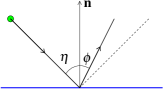
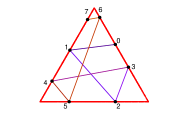
Figure 1: (a) Non-elastic reflection rule; (b) several bounces in an equilateral triangle for $\lambda=0.5$, with collisions numbered in order starting from the initial position $0$.

The phase space of the pinbilliard map is thus contained in $\tilde{M}:=[0,|\gamma|)\times(-\frac{\pi}{2},\frac{\pi}{2})$. In fact, there is a finite number of curves where the map is not defined, consisting of points $(s,\theta)$ located at a vertex of the polygon, or whose trajectories hit a vertex in one iteration, so that an outgoing angle cannot be uniquely defined. The singular locus $\text{Sing}(\lambda)\subseteq\tilde{M}$ of $T_{\lambda}$ consists of all preimages of these curves, for which the dynamics can no longer be continued after some iterate at which the dynamics hits a vertex. We define the phase space $M:=\tilde{M}\setminus\text{Sing}(\lambda)$, the set of points which can be iterated arbitrarily many times. Note that $\text{Sing}(\lambda)$ has zero Lebesgue measure, since it is the union of countably many regular curves.

The main object of interest is the structure of the maximal forward invariant $\Gamma_{\lambda}$ set in $M$, which we refer to as the attractor of $T_{\lambda}$:

$$\Gamma_{\lambda}:=\bigcap_{n\geq 0}T_{\lambda}^{n}(M).$$ (1)

Note that $\Gamma_{\lambda}\subset M=\tilde{M}\setminus\text{Sing}(\lambda)$, and is thus not necessarily compact.

Except in section VII, we shall generally omit reference to the singularity set $\text{Sing}(\lambda)$, but it is always understood that this set must be excluded when discussing the dynamics.

I.1 Structural changes of strange attractors

Figure 2 shows numerically-obtained attractors in phase spacefor pinbilliard dynamics in an equilateral triangle of side length $1$, for several values of $\lambda$. We see that trajectories from almost all initial conditions are observed to accumulate on fractal strange attractors. The main goal of this paper is the explanation of this phenomenology. The main structural changes observed are the following.

For sufficiently small $\lambda$, in fact $\lambda<\frac{1}{3}$, the attractor is a Cantor set of lines, which “thickens” as $\lambda$ increases. For larger values of $\lambda$, triangular-shaped gaps begin to appear in the attractor (b), which become larger as $\lambda$ increases. Afterwards, around $\lambda\simeq 0.68$, the complete horizontal lines visible in the central bands of the attractor break up (c), which we refer to as band splitting. Soon thereafter, round $\lambda\simeq 0.7$, there is band merging to form just three bands (d). These bands shrink as $\lambda$ increases, concentrating around three angle values (e). Finally, for $\lambda\simeq 0.98$ and above, the attractor breaks into three distinct transitive regions (f). The enhanced online multimedia version of this figure shows the evolution of the attractor for all values of $\lambda$. These phenomena will be analyzed in turn in subsequent sections.

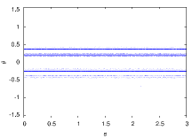
(a) $\lambda=0.3$

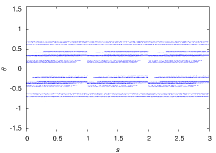
(b) $\lambda=0.5$

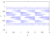
(c) $\lambda=0.68$

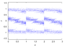
(d) $\lambda=0.8$

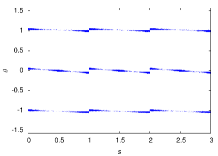
(e) $\lambda=0.95$

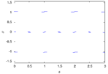
(f) $\lambda=0.98$

Figure 2: Phase space of pinbilliard dynamics in the equilateral triangle, depicting the main structural changes observed in the strange attractor as the contraction parameter $\lambda$ is varied. Each figure except (f) shows a single orbit of length $10^{5}$ starting from a random initial condition, after a transient of $10^{4}$ iterates were discarded to reach the asymptotic attractor. In (f), three such orbits are shown. (Enhanced online.)

I.2 Main theorem for $\lambda<\textstyle\frac{1}{3}$

For $\lambda<\textstyle\frac{1}{3}$, we are able to characterise the dynamics completely via a symbolic model:

Theorem 1 (Main Theorem).

Let $0<\lambda<\textstyle\frac{1}{3}$. Then the attractor $\Gamma_{\lambda}$ of the pinball billiard map in the equilateral triangle is a transitive invariant set and is homeomorphic to $[0,3]\times C\setminus\text{Sing}(\lambda)$, where $C$ is a Cantor set in $\mathbf{R}$. Moreover, there is an invariant ergodic measure on $\Gamma_{\lambda}$, which is absolutely continuous with respect to the Lebesgue measure on horizontal lines.

Section VII of this paper is devoted to a rigorous proof of the Main Theorem.

Note that since all of these maps, restricted to the attractor, are conjugate to the same model, they are also conjugate to one another, i.e. the one-parameter family of pinbilliards is structurally stable for $\lambda<\frac{1}{3}$.

II Equilateral triangle

For the pinbilliard map that we will study, we consider an equilateral triangle of side length $1$. The possible phase space coordinates are then $\tilde{M}=(0,3)\times(-\textstyle\frac{\pi}{2},\textstyle\frac{\pi}{2})$, which we split into $\cup_{i=0}^{2}M_{i}$, where $M_{i}:=(i,i+1)\times(-\textstyle\frac{\pi}{2},\textstyle\frac{\pi}{2})$ is the part of phase space corresponding to the side $i$, with arc length in $(i,i+1)$. (Note that the dynamics is not defined for phase space points whose arc-length parameter sits on a vertex, so these points are automatically excluded from the phase space.) When $i$ denotes a side of the triangle, it must be read modulo $3$, i.e. $i\in\mathbf{Z}_{3}$. In these coordinates, we will refer to vertical and horizontal intervals as being lines in phase space with constant first or second coordinate, respectively.

II.1 Discontinuity curves

Key objects in billiards with piecewise-smooth boundary are the discontinuity curves, which consist of those phase space points that are mapped to a vertex. For the equilateral triangle, the discontinuity curve consists of points $(s,\delta(s))\in M$ with

$$\delta(s):=\arctan\left(\frac{1+2(\lfloor s\rfloor-s)}{\sqrt{3}}\right),$$ (2)

where $\lfloor s\rfloor$ denotes the integer part of $s\geq 0$. The function $\delta$ is independent of $\lambda$, and has image $(-\frac{\pi}{6},\frac{\pi}{6})$. As we shall see, this curve splits each $M_{i}$ into two parts $M^{+}_{i}$ and $M^{-}_{i}$, which are the domains of continuity of $T_{\lambda}$; see figure 3.

Since the geometry of the equilateral triangle is sufficiently simple, we can compute explicitly the angular coordinate of $T_{\lambda}$ in terms of two affine maps:

$$T_{\lambda}(s,\theta)=\left\{\begin{array}[]{l}(\,\cdot\,,\varphi_{+1}(\theta))\qquad\text{ if }\quad\theta>\delta(s),\\ (\,\cdot\,,\varphi_{-1}(\theta))\qquad\text{ if }\quad\theta<\delta(s),\end{array}\right.$$ (3)

where the functions $\varphi_{\pm 1}:\mathbf{R}\to\mathbf{R}$ are defined by

$$\varphi_{\pm 1}(\theta):=\lambda\left(\pm\textstyle\frac{\pi}{3}-\theta\right).$$ (4)

To see this, note that from a starting point $(s,\theta)\in M$, on the side $i:=\lfloor s\rfloor$ of the triangle, there are only two possible types of bounce, depending on $\theta$: a right bounce, on side $i+1$, or a left bounce on side $i-1$; these possibilities are separated by the point $(s,\delta(s))$ that hits the vertex. A straightforward computation verifies that the angular coordinate after the next collision is given by $\phi_{z}(\theta)$, where the sign $z\in\{+1,-1\}$ denotes a right or left bounce, according to the sign of the angle $\pm\frac{\pi}{3}$ between the sides before and after the bounce.

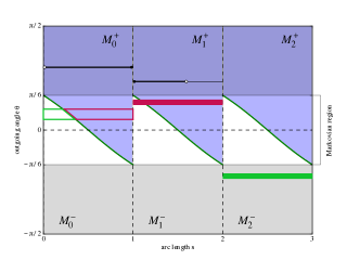
Figure 3: Schematic picture of the phase space of the equilateral triangle, showing the discontinuity lines (solid curved lines) and the resulting domains of continuity $M^{\pm}_{i}$ (shaded and empty). The Markovian region is shown, in addition to a rectangle (green and red open boxes) together with its images (green and red solid rectangles). The horizontal line shows the non-Markovian dynamics, with the open and closed circle indicating the orientation-reversing feature. The dashed vertical lines indicate the positions of the vertices.

The form of $T_{\lambda}$ in (3) implies that locally, horizontal intervals in phase space are mapped onto other horizontal intervals with in general different angles, given by projections along a fixed direction from one side to another.

II.2 Derivative

To calculate expansion and contraction properties of the pin billiard map $T_{\lambda}$, it is necessary to calculate its derivative at a point $(s_{0},\theta_{0})$. The expression for this obtained for a general geometryMarkarian, Pujals, and Sambarino (2010) reduces for polygonal billiard tables, which have only flat boundary components, to

$$D_{(s_{0},\theta_{0})}T_{\lambda}=-\left(\begin{array}[]{ccc}A&B\\ 0&\lambda\end{array}\right),\quad\text{ with}\quad A=\frac{\cos\theta_{0}}{\cos\eta_{1}},\quad B=\frac{t_{0}}{\cos\eta_{1}};$$ (5)

$t_{0}$ denotes the distance between bounces in the billiard table and $\eta_{1}$ the incoming angle at the next collision, as in sec. I.

The upper-triangular structure of the derivative of $T_{\lambda}$ implies that horizontal tangent vectors of the form $v=(a,0)$ are mapped back into horizontal tangent vectors with different base point.

II.3 Periodic orbits

Billiard maps do not have fixed points, and moreover in polygonal billiards neither are there period-$2$ orbits, unless two sides are parallel, in which case there is in fact a whole interval of such orbits. For pinbilliards with our rule, this still holds; thus, any periodic orbit in the equilateral triangle must have period at least $3$.

Lemma 2.

Fix $0<\lambda<1$. Then any periodic orbit of $T_{\lambda}$ is hyperbolic of saddle type.

Proof.

Consider a periodic point $(s_{0},\theta_{0})$ with period $n\geq 3$ and orbit $(s_{j},\theta_{j}):=T_{\lambda}^{j}(s_{0},\theta_{0})$ for $j=1,\ldots,n$. The periodicity implies that $\theta_{n}=\theta_{0}$.

The derivative $D_{(s_{0},\theta_{0})}T_{\lambda}^{n}$ is an upper-triangular matrix with eigenvector $(1,0)$. The absolute value of the corresponding eigenvalue is

$$\mu_{n}:=\frac{\cos\theta_{0}}{\cos\eta_{n}}\prod_{i=1}^{n-1}\frac{\cos\theta_{i}}{\cos\eta_{i}}=\frac{\cos\theta_{0}}{\cos\eta_{n}}\prod_{i=1}^{n-1}\frac{\cos\lambda\eta_{i}}{\cos\eta_{i}},$$ (6)

where $\eta_{i}$ is the incoming angle at the $i$th collision. The left-hand side follows from the chain rule and eq. (5) after a rearrangement; the equality follows from the pinbilliard collision rule $\theta_{i}=-\lambda\eta_{i}$, and using the fact that $\cos$ is an even function. Finally, we have $\cos\theta_{0}/\cos{\eta_{n}}=\cos(\lambda\eta_{n})/\cos(\eta_{n})$, so that $\mu_{n}=\prod_{i=1}^{n}[\cos(\lambda\eta_{i})/\cos\eta_{i}]>1$. Thus the line spanned by $(1,0)$ is the unstable eigenspace of the periodic orbit.

Since the product of matrices of this form along the periodic orbit is also upper-triangular, its determinant is equal to the product of its diagonal entries and is also equal to the product of its eigenvalues. The other eigenvalue is thus $\lambda^{n}<1$. Hence, there is one expanding and one contracting direction, and thus the periodic orbit is hyperbolic of saddle type. ∎

Note that this result holds for any periodic orbit of any polygonal pinball billiard, except the period-$2$ orbits mentioned above.

II.4 Distinguished 3-periodic orbits

For elastic billiard dynamics in an equilateral triangle, there are two distinguished period-$3$ orbits, formed by the median triangle and an orientation. It turns out that we may continue these period-$3$ orbits for pinbilliard dynamics for all $\lambda<1$. They maintain their rotational symmetry and we have the following lemma:

Lemma 3.

There are two hyperbolic period-$3$ orbits of saddle type for any $\lambda\in(0,1)$. Their local unstable manifolds are horizontal lines.

Proof.

The rotational symmetry of the distinguished period-$3$ orbit suggests that the outgoing angle must be a fixed point $\theta_{*}$ of the angular dynamics, so that $\varphi_{+1}(\theta_{*})=\theta_{*}$. It is a straightforward computation that the unique solution is $\theta_{*}:=\theta_{*}(\lambda):=\frac{\pi}{3}\frac{\lambda}{\lambda+1}=\frac{\pi}{3}(\lambda-\lambda^{2}+\lambda^{3}-\cdots)$. In fact, $\varphi_{-1}(-\theta_{*})=-\theta_{*}$ is the counterpart with reversed orientation.

A simple trigonometric calculation using the rotational symmetry of the period-$3$ orbit shows that the point $(s_{3}(\lambda),\theta_{*}(\lambda))$ with

$$s_{3}(\lambda):=\frac{2}{\sqrt{3}\tan(\theta_{*})+3},$$ (7)

is periodic of period $3$ for $T_{\lambda}$.

The previous Lemma then shows that this period-$3$ orbit is always hyperbolic.

To see that the local unstable manifold of the period-$3$ point is a horizontal interval, let $J\subset[0,3]\times\{\theta_{*}\}$ be a small horizontal interval that contains the period-$3$ point. Then $T_{\lambda}^{3}(J)\supset J$, so $J$ is a local unstable manifold of the period-$3$ point. ∎

III Markovian region and complete symbolic dynamics

We shall use the following feature of billiard dynamics in an equilateral triangle: Let $J_{\theta}$ be a horizontal interval which covers one side of the triangle:

$$J_{\theta}:=(i,i+1)\times\{\theta\}\subset M_{i},$$

with $i=0$, $1$ or $2$. There are two possibilities for the structure of the image $T_{\lambda}(J)$, depending on the value of $\theta$: either it is a single horizontal interval or a union of two horizontal intervals, depending on whether the projection in the direction $\theta$ of the side $i$ of the triangle does or does not hit a vertex; see fig. 4.

When $|\theta|>\textstyle\frac{\pi}{6}$, the image $T_{\lambda}(J)$ is a horizontal interval contained in $M_{j}$, where $j$ corresponds to the previous or next side in the table, depending on the sign of $\theta$; and $T_{\lambda}(J)$ is linearly contracted by a factor that depends only on $\theta$ (and not on $\lambda$), and which tends to $1$ as $|\theta|\to\textstyle\frac{\pi}{6}$.

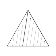
(a) Markovian

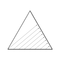
(b) Non-Markovian

Figure 4: Images of horizontal intervals: (a) Markovian case, in which the other two complete sides are covered and there is linear expansion; (b) non-Markovian case, in which only one partial side is covered, and there is linear contraction.

On the other hand, when $|\theta|<\textstyle\frac{\pi}{6}$ the situation is very different. The interval $J$ is now split by the discontinuity curve $\delta$, and hence its image consists of two horizontal intervals, each of which completely covers its corresponding side $j\pm 1$. Moreover, each is linearly expanded and maps across the whole horizontal extent of one of the other two sides. For this reason we call the subset $[0,3]\times(-\textstyle\frac{\pi}{6},\textstyle\frac{\pi}{6})\subset M$ the “Markovian region”. Note that these geometrical properties in the Markovian region in no way depend on $\lambda$.

The key observation is now that when $\lambda<\textstyle\frac{1}{3}$, the image $T_{\lambda}(M)$ of the whole phase space is in fact contained in the Markovian region, and hence, roughly speaking, we can obtain a good partition in terms of future itineraries – i.e., whether the bounce is a left or right bounce at each iteration. This partition is described precisely in section VII.1.

III.1 Angular dynamics

The combinatorics of the horizontal intervals described in the introduction of this section depend on the dynamics of the angular coordinate, which we proceed to study in this section.

The form of the maps $\phi_{\pm}$ in (4) leads us to consider the following geometric series with random signs. Let $0<\lambda<1$ and consider the following subset of real numbers:

$$C(\lambda):=\left\{\frac{\pi}{3}\displaystyle\sum_{n=1}^{\infty}z_{n}\lambda^{n}:z_{n}\in\{1,-1\}\,\forall n\geq 1\right\}.$$ (8)

We show in section VII that $C(\lambda)$ is a Cantor set for $\lambda<\frac{1}{2}$.

Suppose that we are given an angle $\theta\in C(\lambda)$, that is $\theta=\frac{\pi}{3}\sum_{n=1}^{\infty}z_{n}\lambda^{n}$ for some choice of signs $z_{n}\in\{+1,-1\}$. Then $\phi_{\pm}(\theta)\in C(\lambda)$. In fact,

$$\varphi_{\pm 1}(\theta)=\frac{\pi}{3}\left(\pm\lambda-\sum_{n=2}^{\infty}z_{n-1}\lambda^{n}\right).$$ (9)

Thus the images $\varphi_{\pm 1}(C(\lambda))\subset C(\lambda)$ for both maps $\varphi_{\pm 1}$, and hence

$$T_{\lambda}([0,3]\times C(\lambda))\subset[0,3]\times C(\lambda),$$

(except for points in $\text{Sing}(\lambda)$, where $T_{\lambda}$ is not defined). Thus a good candidate for an invariant set is that it be contained in the set $[0,3]\times C(\lambda)$, which for $\lambda<\frac{1}{3}$ is a Cantor set of horizontal lines, and this corresponds with the pictures of the computed attractor shown in fig. 2(a). In section VII we rigorously prove that the attractor is indeed precisely $[0,3]\times C(\lambda)$ without the singularity set.

III.2 Periodic orbits

The geometric series that arise in the angular dynamics allow us to find periodic orbits with period $m$ and particular itinerary. That is, suppose we are given a word $w$ of length $m\geq 3$, given by $w=(w_{j})$ with $w_{j}\in\{+1,-1\}$ for $j=1,\ldots,m$. Each $w_{j}$ specifies which kind of bounce, left or right, occurs at the $j$th iteration. If $(s_{w},\theta_{w})$ is to be a periodic orbit of period $m$ with this itinerary, then its angle must satisfy the equation

$$\theta_{w}=\varphi_{w_{m}}\circ\cdots\circ\varphi_{w_{1}}(\theta_{w})=\frac{\pi}{3}\sum_{j=1}^{m}(-1)^{j-1}w_{m-j+1}\lambda^{j}+(-\lambda)^{m}\theta_{w},$$ (10)

where the second equality gives the explicit formula for the composition. Solving for $\theta_{w}$ gives

$$\theta_{w}=\frac{\pi}{3}\left[\sum_{j=1}^{m}(-1)^{j-1}w_{n-j+1}\lambda^{j}\right]\,\left[\sum_{k=0}^{\infty}(-\lambda)^{km}\right],$$

since the infinite series equals $[1-(-\lambda)^{m}]^{-1}$.

Setting $b_{km+j}:=(-1)^{km+j-1}w_{m-j+1}$ for any $j=1,\ldots,m$ and $k\in\mathbf{N}$, we conclude that

$$\theta_{w}=\sum_{n=1}^{\infty}b_{n}\lambda^{n},$$

and hence $\theta_{w}\in C(\lambda)$.

When $\lambda<\textstyle\frac{1}{3}$, all iterations of the interval $[0,1]\times\{\theta_{w}\}$ are contained in the Markovian region. Hence we can partition this interval according to its future itineraries. Selecting the partition element $J_{w}$ corresponding to the itinerary $w$, we have $T_{\lambda}^{m}(J_{w})\supset J_{w}$, so that there is a periodic orbit with periodic itinerary $(w,w,w,\ldots)$.

This is the basis of the argument for the rigorous proof of the Main Theorem presented in section VII. Here we exhibit in fig. 5 two examples of periodic orbits found numerically using this method.

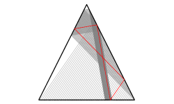
(a) Period 4

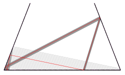
(b) Period 5

Figure 5: Periodic orbits (red) in the equilateral triangle for pinbilliard dynamics with $\lambda=0.3$: (a) period-$4$ orbit with itinerary $(+1,+1,-1,-1)$; (b) period-$5$ orbit with itinerary $(+1,+1,+1,-1,+1)$. The light grey lines show the complete regions with the same itinerary and angles.

IV Non-accessible regions in phase space

As discussed in the previous section, for $\lambda\leq\frac{1}{3}$ the attractor consists of complete horizontal lines, so that for a given angle $\theta\in C(\lambda)$, (almost) all positions in $[0,3]\times\{\theta\}$ are attained in the attractor. For $\lambda>\frac{1}{3}$, some of these horizontal lines are cut, giving rise to gaps, located close to the table vertices, that no longer form part of the attractor; see fig. 2(b). These regions are approximately triangular in shape, and change form as $\lambda$ varies.

To explain this phenomenon, we say that a angle point $(s,\theta)$ is non-accessible if $(s,\theta)\notin T_{\lambda}^{n}(M),$ for some iterate $n$. For example, $(0,3)\times\left(\frac{\lambda\pi}{2},\frac{\pi}{2}\right)$ is such a non-accessible region for $n=1$, along with its mirror image with negative angular coordinate. Obviously, such non-accessible regions cannot belong to the attractor.

To avoid cumbersome notation, we will mainly work with intervals of angles and their dynamics under $\phi_{\pm 1}$. We denote by $N:=(-\frac{\pi}{2},\frac{\pi}{2})$ the whole range of available angles, and by $K:=(-\frac{\pi}{6},\frac{\pi}{6})$ the angles corresponding to the Markovian region. Furthermore, given an interval $L=(\ell_{1},\ell_{2})$ and a scalar $\rho$, we denote $\rho L:=(\rho\ell_{1},\rho\ell_{2})$. Recall that $\phi_{\pm 1}$ are affine maps of $\mathbf{R}$ that depend on $\lambda$.

Simple calculations show that the images $\phi_{+1}(K)=(\lambda\frac{\pi}{6},\lambda\frac{\pi}{2})$ and $\phi_{-1}(K)=-\phi_{+1}(K)$ are disjoint intervals, both contained in $\lambda N$, and the gap between them is $\lambda K$; that is, we have $\lambda N=\phi_{+1}(K)\cup\lambda K\cup\phi_{-1}(K)$, together with two points at the boundaries of the intervals.

If $\lambda<\frac{1}{3}$, then we have that $\lambda N\subset K$, and hence we can conclude that the strip $(0,3)\times\lambda K\subset M$ is a non-accessible region, since it is not contained in $T_{\lambda}(M)$. Iterating this procedure gives rise to the Cantor set $C(\lambda)$ discussed in the previous section.

When $\lambda>\frac{1}{3}$, we now have the opposite case: $\lambda N\supset K$, so there are points that may enter the middle gap. Since we have studied the images of points inside $K$ under the action of $\phi_{+1}$ and $\phi_{-1}$, it remains to study the images of $\lambda N\setminus K$.

Let $\alpha:=\phi_{+1}(+\lambda\frac{\pi}{2})=\textstyle\frac{\pi}{6}(2\lambda-3\lambda^{2})$; by symmetry, we have $\phi_{-1}(-\lambda\frac{\pi}{2})=-\alpha$. For $\lambda>\frac{1}{3}$, we have $\alpha<\lambda\frac{\pi}{6}$, so that the image of $\lambda N\setminus K$ covers part of the previously-found gap. When $\alpha=0$, at $\lambda=\frac{2}{3}$, the gap is completely covered by this image.

The images of the interval $\lambda N\setminus K$ consist of two symmetric intervals, $L:=(\alpha,\lambda\frac{\pi}{6})$ and $-L$. It is, however, necessary to study in more detail the position coordinate of the image under $T_{\lambda}$ of the strip $(0,3)\times L$, since $\lambda N\setminus K$ is no longer in the Markovian region, and so the image of horizontal intervals of the form $(i,i+1)\times\theta$ do not completely cover a side.

We thus only need to study the image of the rectangle $R:=[0,1]\times(\frac{\pi}{6},\lambda\frac{\pi}{2})\subset M^{+}_{0}$, where $M^{+}_{0}$ is in the domain of $\phi_{+1}$. We have already shown that the image $T_{\lambda}(R)\subset[1,2]\times L$.

In order to obtain a better notion of the shape of the image, we have to be careful about the images of each of the four sides of the rectangle $R$. The map $T_{\lambda}$ is, of course, not defined on vertical sides, but we can take its continuous extension.

The bottom side of $R$, given by $(0,1)\times\{\frac{\pi}{6}\}$, is mapped onto the line $(1,2)\times\{\lambda\frac{\pi}{2}\}$, while the top side, $(0,1)\times\{\lambda\frac{\pi}{2}\}$, is mapped onto a sub-interval $(1,\ell)\times\{\alpha\}$, reversing the orientation. The point $\ell=\ell(\lambda)$ corresponds to the point where a ball hits the triangle’s boundary if it starts on the vertex $0$ with angle $\lambda\frac{\pi}{2}$.

For the right side of $R$, it is necessary to consider vertical lines $\{1-\epsilon\}\times(\frac{\pi}{6},\lambda\frac{\pi}{2})$ for small $\epsilon>0$, since the image is not actually defined for the right side of $R$. It is clear that the projection on the angular coordinate of the image covers the whole interval $\left(\alpha,\lambda\frac{\pi}{6}\right)$, since the angles do not depend on the position $s$ on the table. Furthermore, as $\epsilon\to 0$, both ends of the curve converge to the vertex at $s=1$. So the continuous extension of $T_{\lambda}$ maps the right side of the rectangle onto the vertical interval $\{1\}\times\left(\alpha,\lambda\frac{\pi}{6}\right)$.

Finally, the left side of $R$, given by $\{0\}\times(\frac{\pi}{6},\lambda\frac{\pi}{2})$, is mapped to a curve joining the point $(2,\lambda\frac{\pi}{2})$ and the point $(\ell,\alpha)$. In fact, this curve is given by $\gamma(t):=(\ell(t),\phi_{+1}(t))$ for $t\in(\frac{\pi}{6},\lambda\frac{\pi}{2})$, where

$$\ell(t):=1+\frac{2}{1+\sqrt{3}\tan(t)}.$$ (11)

Note that only the endpoint $\ell=\ell(\lambda\frac{\pi}{2})$, and not the curve itself, depends on $\lambda$.

To summarise, we have shown that $T_{\lambda}(M_{0}^{+})$ is contained in $M_{1}$ in the region bounded below by the curves $\max\{\alpha,\gamma(t)\}$, and above by the line $\lambda\frac{\pi}{2}$.

The other way that trajectories can be injected into $M_{1}$ is if they come from $M_{2}^{-}$. By symmetry, the relevant image of $M_{2}^{-}$ is bounded by the curves $-\lambda\frac{\pi}{2}$ and $\min\{-\alpha,\gamma(t)\}$. This is shown in figure 6, and explains the presence of the triangular-shaped gaps in the attractor.

As we have seen, when $\lambda>\frac{2}{3}$, the angular parts of the images overlap. In fig. 6(c), we see that the complete images in fact touch. Although this makes possible that the central bands of the attractor join as soon as $\lambda>\frac{2}{3}$, in fact we observe numerically that this occurs later, around $\lambda\simeq 0.7$. This can be understood by tracing the evolution of the non-accessible regions in time and finding the limits of the region around $\theta=0$ which is correspondingly excluded from the attractor.

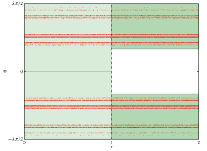
(a) $\lambda=0.3$

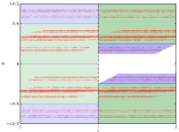
(b) $\lambda=0.5$

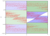
(c) $\lambda=0.75$

Figure 6: Action of $T_{\lambda}$ on $\lambda M_{0}$ for different values of $\lambda$. The Markovian region is shaded in green and the non-Markovian region in blue. Darker shading is used for the images, shown for $s\in(1,2)$; lighter shading is used for the domain, shown for $s\in(0,1)$. The attractor is shown in red dots.

V Isolation of period-3 orbit from the attractor

Recall from figure 2(b) that a splitting of the central bands of the attractor is observed around $\lambda\simeq 0.68$. This is related to the local stable and unstable manifolds of the distinguished period-$3$ orbit discussed in section II.4.

Figure 7 shows the period-$3$ orbit together with the attractor. From the figure, we see that the period-$3$ orbit is embedded in the attractor before the bands split, and in particular that its local unstable manifold is a complete horizontal line contained in the center of the band. After the band splits, however, the period-$3$ orbit becomes isolated from the strange attractor, and there is no longer such a central line.

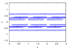
(a) $\lambda=0.5$

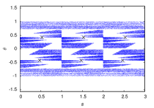
(b) $\lambda=0.68$

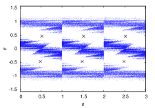
(c) $\lambda=0.8$

Figure 7: Phase space of pinbilliard dynamics in the equilateral triangle, with the period-$3$ orbits shown as crosses.

This phenomenon is due to a homoclinic bifurcation: for $\lambda=0.55$, the stable and unstable manifolds of the period-$3$ meet, forming a homoclinic point, as shown in fig. 8(a). Thus any neighbourhood of the period-$3$ orbit contains recurrent points, and hence the period-$3$ point is not isolated from the dynamics.

By $\lambda\simeq 0.75$ the stable and unstable manifolds no longer meet, and this recurrence is destroyed, allowing the period-$3$ orbit to become isolated.

To obtain these figures, the unstable manifold is obtained by iterating a local horizontal interval around the period-$3$ point. The stable manifold, on the other hand, is approximated using the following escape-time algorithm. For a given point in phase space to belong to the local stable manifold of the period-$3$ orbit, its future iterates must follow the same dynamics as the period-$3$ orbit, e.g. only have right bounces. We thus iterate each point in a grid on the domain a certain number $n$ of times; if the point has only right bounces up to this time, then the initial condition is marked as forming part of the approximate local stable manifold of order $n$. Of course, this does not give the precise shape of the stable manifold, but rather a region in which it must be contained. In particular, this guarantees that there is no homoclinic point if the unstable manifold does not cross this region.

This phenomenon also provides evidence of the relation (Chernov and Markarian, 2003, Section III.3) between expansion in the unstable direction and fractioning due to the set $\text{Sing}(\lambda)$. The expansion in the unstable direction of the period-$3$ orbit is given by $[\frac{\cos(\lambda\theta_{*})}{\cos(\theta_{*})}]^{3}$, which decreases as $\lambda$ increases.

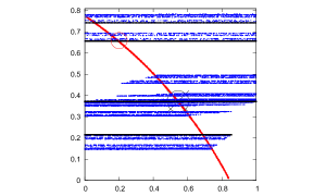
(a) $\lambda=0.55$

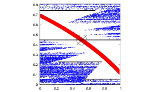
(b) $\lambda=0.75$

Figure 8: The region $M_{0}$ with non-negative angles, showing the strange attractors (blue points), one point in the period-$3$ orbit (crossed circle), several iterations of the unstable manifold of the periodic point (thick black line), and a region in which its local stable manifold must be contained (red area) for (a) $\lambda=0.55$ and (b) $\lambda=0.75$. In (a), there is a homoclinic point (intersection of the stable and unstable manifolds), marked with a small red circle. A number of iterations $n=30$ was used.

VI Non-transitive behaviour close to $\lambda=1$

For $\lambda\simeq 0.98$, we observe that there are three distinct transitive parts of the attractor, i.e. such that it is impossible to jump from one to the other; see fig. 9.

The reason for this phenomenon is the following. After enough iterations, the system arrives close to a vertex, with an angle close to $\frac{\pi}{3}$, so that it collides with the opposite side at an almost perpendicular angle, and is reinjected back into the same corner. This acts as a trapping region which prevents the system from escaping to one of the other parts of the attractor.

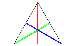
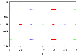
Figure 9: Three non-communicating transitive parts of the attractor, shown in different colors for $\lambda=0.98$, in (a) configuration space and (b) phase space.

Figure 10: Basins of attraction of the three transitive parts of the attractor, shown in three different colors, exhibiting a fractal basin boundary. (a) Region around one part of one of the transitive parts of the attractor, centered at $(0.5,0)$. (b) Detail of the basin boundary.

In 10 the basins of attraction of each of the three symmetrical copies of this region are shown, indicating a fractal basin boundary structure.

VII Proof of Main Theorem

In this section we give a rigorous proof of the Main Theorem. This will be done in two parts, treating separately the topological and the ergodic properties, although both are consequences of the existence of a topological conjugacy of the pinball billiard map in the attractor with a symbolic dynamics model.

Let us recall that the attractor of $T_{\lambda}$ (or maximal forward invariant set in $M$) is defined by $\Gamma_{\lambda}:=\cap_{n\geq 0}T_{\lambda}(M)\subset M$. Roughly speaking, the symbolic model will be a shift-like map in the space of bi-infinite sequences of $\pm 1$, but interchanging signs in a certain part of the sequence at each iteration; this map is defined in eq. (14). This map possesses a natural ergodic measure which will be pulled down to an invariant, ergodic measure for the pinball billiard map using the above-mentioned conjugation.

The Markovian property that guarantees uniform expansion along certain horizontal intervals is the cornerstone in the construction of the conjugation, discussed in sec. III and constructed in section VII.1 below. In some cases, for instance for $0<\lambda<\frac{1}{3}$, the attractor is contained in the region where this property holds, allowing us to prove the existence of a dense orbit.

It is interesting that the set of geometric series with random signs is intimately related with the action of the collision rule of the pinball billiard map on the angular coordinate.

Let $0<\lambda<1$ and recall the set $C(\lambda)$ defined in (8):

$$C(\lambda):=\left\{\frac{\pi}{3}\sum_{n=1}^{\infty}z_{n}\lambda^{n}:z_{n}\in\{1,-1\}\,\forall n\geq 1\right\}.$$

This is a subset of the interval $\frac{\pi}{3}[-\frac{\lambda}{1-\lambda},\frac{\lambda}{1-\lambda}]$. It is a Cantor set if $\lambda<\textstyle\frac{1}{2}$, and all numbers in $C(\lambda)$ then have a unique expression in terms of a signed geometric series, whereas for $\lambda\geq\textstyle\frac{1}{2}$ it is a full interval, which grows to fill up $\mathbf{R}$ as $\lambda\to 1$.

To prove the Cantor structure of this set, note that if $\lambda<\textstyle\frac{1}{2}$ then for each integer $m\geq 1$ we have

$$\delta_{m}:=\frac{\pi}{3}\lambda^{m}-\frac{\pi}{3}\sum_{j=m+1}^{\infty}\lambda^{j}=\frac{\pi}{3}\,\frac{1-2\lambda}{1-\lambda}\lambda^{m}>0.$$

Hence, there are no points of $C(\lambda)$ in any open interval of the form $(s-\delta_{m},s+\delta_{m})$, for any partial sum $s=\frac{\pi}{3}\sum_{j=1}^{m-1}\pm\lambda^{j}$. In the same fashion, the length of each bounded connected component of the complement of the union of these intervals is of order $\lambda^{m+2}$.

On the other hand, if $\lambda<\textstyle\frac{5}{6}$ then $C(\lambda)\subset[-\textstyle\frac{\pi}{2},\textstyle\frac{\pi}{2}]$. Recall that the set $C(\lambda)$ is invariant under both maps $\varphi_{\pm 1}$, i.e. $\varphi_{\pm 1}(C(\lambda))\subset C(\lambda)$.

To observe the relation between the geometric series and the pinbilliard, consider the topological space

$$\Sigma_{2}^{+}:=\{(z_{n}):z_{n}\in\{1,-1\}\,\forall n\geq 1\},$$

with the standard product topology, and the modified shift transformation $-\sigma:\Sigma_{2}^{+}\to\Sigma_{2}^{+}$ given by $-\sigma((z_{n})):=(-z_{n+1})$. In these terms, if $0<\lambda<\textstyle\frac{1}{2}$, then both maps $\varphi_{\pm 1}$ are branches of the inverse $E_{\lambda}^{-1}(-\sigma(z))$, where the map $E_{\lambda}:\Sigma_{2}^{+}\to C(\lambda)$ is defined by

$$E_{\lambda}(z):=\frac{\pi}{3}\sum_{n=1}^{\infty}z_{n}\lambda^{n}.$$ (12)

The condition $0<\lambda<\textstyle\frac{1}{2}$ guarantees that $E_{\lambda}^{-1}:C(\lambda)\to\Sigma_{2}^{+}$ is well-defined.

On the other hand, to any point in phase space having an entire well-defined future orbit there corresponds a sequence $(w_{n})\in\Sigma_{2}^{+}$, such that $w_{n}=+1$ if the $n$th iterate is a right bounce, or $w_{n}=-1$ if it is a left bounce. So, if $(s_{0},\theta_{0})\in M\setminus\text{Sing}(\lambda)$, then for any $n\geq 1$ we have $T^{n}(s_{0},\theta_{0})=(s_{n},\theta_{n})$, where

$$\theta_{n}=\varphi_{w_{n}}\circ\cdots\circ\varphi_{w_{1}}(\theta_{0})=\frac{\pi}{3}\sum_{j=1}^{n}(-1)^{j-1}w_{n-j+1}\lambda^{j}+(-\lambda)^{n}\theta_{0}.$$ (13)

In this way, we can define the function $\mathcal{I}:\Gamma_{\lambda}\to\Sigma_{2}^{+}$ by $\mathcal{I}(P):=(w_{n})\in\Sigma_{2}^{+}$ for $P\in\Gamma_{\lambda}$. If a point hits a vertex of the table at some iterate $k\geq 1$ then one cannot compute its itinerary after the $k$th step. In this case, we take the convention that the tail of the itinerary is either $w_{k+j}=(-1)^{j}$ or $(-1)^{j+1}$, for $j\geq 1$.

Recall that for any $0<\lambda<1$ we have $T_{\lambda}(M)\subset(0,3)\times(-\lambda\textstyle\frac{\pi}{2},\lambda\textstyle\frac{\pi}{2})$, and note that if $0<\lambda<\textstyle\frac{1}{3}$ then $C(\lambda)\subset(-\lambda\textstyle\frac{\pi}{2},\lambda\textstyle\frac{\pi}{2})$. For such $\lambda$, the attractor $\Gamma_{\lambda}$ inherits the geometry of $C(\lambda)$, as shown in the following lemma.

Lemma 4.

If $0<\lambda<\textstyle\frac{1}{3}$ then $\Gamma_{\lambda}\subset(0,3)\times C(\lambda)$.

Proof.

Consider any point $(q,\theta)\in\Gamma_{\lambda}$. Then there exists a point $(p_{0},\theta_{0})\in M\setminus\text{Sing}(\lambda)$, and an increasing sequence of integers $n_{k}\to\infty$, such that $(p_{n_{k}},\theta_{n_{k}}):=T_{\lambda}^{n_{k}}(p_{0},\theta_{0})\to(q,\theta)$ as $k\to\infty$. Using the expression in (13), we have, for any $k\geq 1$, that

$$\left|\theta_{n_{k}}-\frac{\pi}{3}\left(\sum_{j=1}^{n_{k}}(-1)^{j-1}w_{n_{k}-j+1}\lambda^{j}+\sum_{j=n_{k}+1}^{\infty}\pm\lambda^{j}\right)\right|$$

$$<\lambda^{n_{k}}\frac{\pi}{2}+\frac{\pi}{3}\frac{\lambda^{n_{k}+1}}{1-\lambda}<C\lambda^{n_{k}},$$

for some positive constant $C$ and any selection of $\pm 1$ in the series on the right-hand side. Thus $\theta\in C(\lambda)$. ∎

VII.1 Region with a Markovian property

The discontinuity curve $\delta$, defined in (2), does not depend on the parameter $\lambda$, and its image is contained in the rectangle $(0,3)\times(-\textstyle\frac{\pi}{6},\textstyle\frac{\pi}{6})$. Furthermore, phase space is naturally partitioned into horizontal intervals of the form $J(i,\theta):=(i,i+1)\times\{\theta\}$ for $i\in\mathbf{Z}_{3}$ and $\theta\in(-\textstyle\frac{\pi}{2},\textstyle\frac{\pi}{2})$. We denote this partition by $\mathcal{J}$.

We define $\mathcal{J}_{0}\subset\mathcal{J}$ as $\mathcal{J}_{0}:=\{J(i,\theta)\in\mathcal{J}:|\theta|<\frac{\pi}{6}\}$. The region of phase space covered by $\mathcal{J}_{0}$, i.e. the union of all $J(i,\theta)\in\mathcal{J}$ such that $|\theta|<\textstyle\frac{\pi}{6}$, has a non-uniform expanding behavior along horizontal lines. To see this, note that any $J\in\mathcal{J}_{0}$ is partitioned into two non-trivial subintervals $J=J(i,\theta)=L_{\theta}^{i}\cup R_{\theta}^{i}$, where $L_{\theta}^{i}:=(i,d_{\theta}]\times\{\theta\}$ and $R_{\theta}^{i}:=[d_{\theta},i+1)\times\{\theta\}$, and $d_{\theta}$ is the first coordinate of the intersection point of the image of the curve $\delta$ with the interval $J(i,\theta)$. So, the set $\mathcal{S}=\{L_{\theta}^{i},\,R_{\theta}^{i}:i\in\mathbf{Z}_{3},|\theta|<\textstyle\frac{\pi}{6}\}$ is a refinement of $\mathcal{J}_{0}$, such that any atom of $\mathcal{S}$ is almost contained in some continuity domain of $T_{\lambda}$. Precisely, given any $S\in\mathcal{J}$, if we denote by $\text{int}(S)$ the interval $S$ without its extreme points, then we have that $\text{int}(S)$ is contained in some continuity region of $T_{\lambda}$.

The Markovian property of the partition $\mathcal{J}_{0}$ is the following: for any $S\in\mathcal{S}$, the restriction of $T_{\lambda}|_{\text{int}(S)}$ extends to a continuous and surjective map $f_{S}:S\to J$, for some $J\in\mathcal{J}$. In fact, each of these maps is a linear projection between sides of the triangle, along some fixed direction, and hence affine. Furthermore, for any $S\in\mathcal{S}$ the derivative is constant and can be computed as $(f_{S})^{\prime}=|S|^{-1}>1$, where $|S|$ denotes the length of the interval $S$. Note that $(f_{J(i,\theta)})^{\prime}\to 1$ as $\theta\to\textstyle\frac{\pi}{6}$. These properties do not depend on $\lambda$.

If we fix some $0<\lambda<\textstyle\frac{1}{3}$, then the set $\Gamma_{\lambda}$ is properly contained in the Markovian region. That is, there is $\epsilon>0$ such that

$$\Gamma_{\lambda}\subset(0,3)\times(-\textstyle\frac{\pi}{6}+\epsilon,\textstyle\frac{\pi}{6}-\epsilon)\subset\bigcup_{J\in\mathcal{J}_{0}}J,$$

where equality is excluded.

So for any $S\in\mathcal{S}$ we have that $f_{S}(S)\in\mathcal{J}_{0}$. Moreover, there is a uniform expansion along the horizontal direction: in fact, there is $\rho=\rho(\lambda)>1$ such that $(f_{S})^{\prime}>\rho$, for any $S\subset J(i,\theta)$ such that $|\theta|<\lambda\textstyle\frac{\pi}{2}$.

These properties allow us to describe more precisely the dynamics of the pinbilliard map in terms of symbolic dynamics. Let us first state the following lemma:

Lemma 5.

Fix some $0<\lambda<\textstyle\frac{1}{3}$. For each $(i,\theta)\in\mathbf{Z}_{3}\times C(\lambda)$ there is a continuous map $P(i,\theta):\Sigma_{2}^{+}\to J(i,\theta)\in\mathcal{J}_{0}$ such that $\mathcal{I}\circ P=\text{Id}$.

Proof.

Fix some $0<\lambda<\textstyle\frac{1}{3}$, and consider any$(i,\theta)\in\mathbf{Z}_{3}\times C(\lambda)$. Let $J_{0}=J(i,\theta)\in\mathcal{J}_{0}$. In order to define the map $P(i,\theta):\Sigma_{2}^{+}\to J_{0}$, consider a point $w=(w_{n})\in\Sigma_{2}^{+}$. We take the first $k$ letters of $w$ and will find a closed interval $H_{k}=H(w_{1},\ldots,w_{k})\subset J_{0}$ such that, for any $Q\in H_{k}$, the first $n$ coordinates of $\mathcal{I}(Q)\in\Sigma_{2}^{+}$ are precisely $w_{1},\ldots,w_{k}$. If $\cap_{k}H_{k}\subset J_{0}$ is a unique point, then the map will then be well-defined.

To define these intervals we shall proceed inductively on $k$: Recall that $J_{0}\in\mathcal{J}_{0}$, and so it splits into two subintervals, $J_{0}=L\cup R$, for some $L,\,R\in\mathcal{S}$; then let $H_{1}=R$ if $w_{1}=1$, or $H_{1}=L$ if $w_{1}=-1$. It is easy to see that the first coordinate of $\mathcal{I}(Q)$ is $w_{1}$, for any $Q\in H_{1}$. Notice that $f_{J_{0}}(H_{1})=:J_{1}\in\mathcal{J}_{0}$. Now let us assume that $H_{k-1}\subset J_{0}$ is defined and satisfies

$$J_{k}:=f_{J_{k-1}}\circ\cdots\circ f_{J_{1}}\circ f_{J_{0}}(H_{k-1})\in\mathcal{J}_{0}.$$

Then $J_{k}=L_{k}\cup R_{k}$ for some $L_{k},\,R_{k}\in\mathcal{S}$, and so, in the same way, we can define $H_{k}=(f_{J_{k-1}}\circ\cdots\circ f_{J_{0}})^{-1}(A)$, where either $A=L_{k}$, or $A=R_{k}$, depending on $w_{k}$.

We have that $|H_{k}|\to 0$ as $k\to\infty$. In fact, all $J_{k}=J(\,\cdot\,,\theta_{k})\in\mathcal{J}_{0}$ involved in the construction are such that $|\theta_{k}|<\lambda\textstyle\frac{\pi}{2}<\textstyle\frac{\pi}{6}$, and hence $(f_{J_{k}})^{\prime}>\rho>1$. So $|H_{k}|<\rho^{-k}$, for any $k\geq 1$, and therefore, there is a unique $P=P(i,\theta)(w)\in\bigcap_{k\geq 1}H_{k}$ and we have $\mathcal{I}(P)=w$.

This map is continuous by construction and it is injective at all points, except those with a periodic tail (see the definition of the map $\mathcal{I}$), which correspond to points that eventually hit some vertex of the table, which are mapped to the same points in $J_{0}$. ∎

As a consequence of the construction in the proof of the previous lemma one obtains the following: on any $J:=J(i,\theta)\in\mathcal{J}_{0}$ such that $J\cap\Gamma_{\lambda}\neq\emptyset$, that is $\theta\in C(\lambda)$, any itinerary in $\Sigma_{2}^{+}$ is followed by a unique point in $J$, with exception of those itineraries with periodic tail, which correspond to the same orbit that eventually hits a vertex. In fact, such exceptions correspond to points in the discontinuity set $\text{Sing}(\lambda)$. Hence, $J\subset\Gamma_{\lambda}$, and this proves that $\Gamma_{\lambda}$ is homeomorphic to $(0,3)\times C(\lambda)\setminus\text{Sing}(\lambda)$.

Thus, we can gather together the maps obtained in Lemma 5 to create the following transformation that depends only on $\lambda$:

$$P_{\lambda}:\Sigma_{2}^{+}\times\Sigma_{2}^{+}\times\mathbf{Z}_{3}\to\Gamma_{\lambda};$$

$$P_{\lambda}(w,z,i):=P(i,E_{\lambda}(z))(w).$$

Observe that this map is continuous, and if $(p,\theta)\in(0,3)\times C(\lambda)$ then the inverse of $P_{\lambda}$ is defined by $P_{\lambda}^{-1}(p,\theta)=(\mathcal{I}(p,\theta),E_{\lambda}^{-1}(\theta),\lfloor p\rfloor)$, where $\lfloor p\rfloor$ denotes the integer part of $p$. Hence, $P_{\lambda}$ is a homeomorphism in $P_{\lambda}^{-1}(\Gamma_{\lambda}\setminus\text{Sing}(\lambda))$ and conjugates the pinball billiard map to the following symbolic model:

$$[(w,z),i]\mapsto[(\sigma(w),(w_{1},-z_{1},-z_{2},\ldots)),i+w_{1}],$$ (14)

where $\sigma:\Sigma_{2}^{+}\to\Sigma_{2}^{+}$ is the standard shift, and the addition operation in the last coordinate is in $\mathbf{Z}_{3}$.

This complete description of the dynamics of the pinball map allows us to prove transitivity in $\Gamma_{\lambda}$, as we shall see in the next Lemma.

Lemma 6.

The pinbilliard map $T_{\lambda}|_{\Gamma_{\lambda}}$ is transitive.

Proof.

Take any two non-empty open subsets $U$ and $V$ of $\Gamma_{\lambda}$. We shall prove that there is some $N\geq 0$ such that $T_{\lambda}^{N}(U)\cap V\neq\emptyset$. First note that there is some interval $J_{1}:=J(i_{1},\theta_{1})\in\mathcal{J}_{0}$ such that $J_{1}\cap U$ is a non-trivial interval, since $U$ is open. Now, the construction in the proof of Lemma 5 allows us to say that there is some interval $H_{1}\subset J_{1}\cap U$ and $N_{1}\geq 0$ such that $T_{\lambda}^{N_{1}}(H_{1})=J_{2}\in\mathcal{J}_{0}$. Therefore, there are $(i_{2},\theta_{2})\in\mathbf{Z}_{3}\times C(\lambda)$ such that $J_{2}=J(i_{2},\theta_{2})$.

On the other hand, there is some interval $J(i_{*},\tilde{\theta})\in\mathcal{J}_{0}$, such that $J(i_{*},\tilde{\theta})\cap V\neq\emptyset$ for some $(i_{*},\tilde{\theta})\in\mathbf{Z}_{3}\times C(\lambda)$, since $V$ is open.

Now we claim that for any $\epsilon>0$ there is some $N_{2}\geq 0$ and an interval $H_{2}\subset J_{2}$ such that $T_{\lambda}^{N_{2}}(H_{2})=J_{3}\in\mathcal{J}_{0}$, and hence $J_{3}=J(i_{3},\theta_{3})$ for some $(i_{3},\theta_{3})\in\mathbf{Z}_{3}\times C(\lambda)$, and such that $i_{3}=i_{*}$ and $|\theta_{3}-\tilde{\theta}|<\epsilon$. If this claim holds and we take $\epsilon>0$ small enough, it implies that $T_{\lambda}^{N_{1}+N_{2}}(H_{1})\cap V\neq\emptyset$, proving transitivity.

To get the claim denote $(a_{1},a_{2},\ldots)=E_{\lambda}^{-1}(\tilde{\theta})\in\Sigma_{2}^{+}$. Fix some $k\geq 1$ such that $\lambda^{k+1}<\epsilon$. We will select a point $w\in\Sigma_{2}^{+}$ specifying just the first $k$ coordinates in the following way: let

$$w:=((-1)^{k-1}a_{k},(-1)^{k-2}a_{k-1},\ldots,-a_{2},a_{1},w_{k+1},\ldots)\in\Sigma_{2}^{+}.$$

If we let $z=E_{\lambda}^{-1}(\theta_{2})$, then by the formula in (14) one gets

$$\tau^{k}(w,z,i_{2})=(\sigma^{k}(w)\,,\,(a_{1},\ldots,a_{k},z_{1},\ldots)\,,\,i_{2}+\sum_{s=1}^{k}(-1)^{s-1}a_{s}).$$

Observe that $|\tilde{\theta}-E_{\lambda}(a_{1},\ldots,a_{k},z_{1},\ldots)|<\lambda^{k+1}<\epsilon$. So, in order to obtain the claim it is left to prove that $i_{2}+\sum_{s=1}^{k}(-1)^{s-1}a_{s}=i_{*}\,\text{mod}\,3$. However, this is not always true. For instance, let us assume that they differ by 2. Then, to get the claim we may need to change the itinerary $w$, by adjoining two signs $b_{1}$ and $b_{2}\in\{\pm 1\}$ at the beginning:

$$w=(b_{2},b_{1},(-1)^{k-1}a_{k},(-1)^{k-2}a_{k-1},\ldots,-a_{2},a_{1},\ldots)\in\Sigma_{2}^{+},$$

and iterate $k+2$ times to obtain the claim. In fact,

$$\tau^{k+2}(w,z,i_{2})=\left(\sigma^{k+2}(w)\,,\,(a_{1},\ldots,a_{k},b_{1},b_{2},z_{1},\ldots)\right.,$$

$$\left.i_{2}+\sum_{s=1}^{k}(-1)^{s-1}a_{s}-b_{2}+b_{1}\right).$$

If these numbers differ only by $1$, then the same argument applies by adjoining only one $b_{1}\in\{\pm 1\}$. ∎

This completes the proof of the topological part of Theorem 1.

VII.2 Invariant measure on $\Gamma_{\lambda}$

The space $\Sigma_{2}^{+}\times\Sigma_{2}^{+}\times\mathbf{Z}_{3}$ has a natural probability measure $\mu$, defined on Borel sets, which is invariant under the map in (14). This measure is in fact a Bernoulli measure, and is a product $\mu=\nu\times\nu$, where $\nu$ is the invariant Bernoulli measure for the standard shift $\sigma:\Sigma_{2}^{+}\to\Sigma_{2}^{+}$, weighted in order that $\mu(\Sigma_{2}^{+}\times\Sigma_{2}^{+}\times\{i\})=\textstyle\frac{1}{3}$, for $i\in\mathbf{Z}_{3}$.

On the other hand, one can define a measure $\mu_{\lambda}$ on Borel sets of $\mathbf{R}$ using the maps $E_{\lambda}$, for $0<\lambda<1$, in the following way: given any measurable set $A\subset\mathbf{R}$, let

$$\mu_{\lambda}(A):=\nu(E_{\lambda}^{-1}(A)).$$

Properties of the measure $\mu_{\lambda}$, in particular for which values it is absolutely continuous with respect to Lebesgue measure, have been studied since 1920 by Khintchine and Kolmogoroff Khintchine and Kolmogoroff (1925), and several interesting results have been developed by Erdös, Garsia, Pollicott and Solomyak during the 20th century; see Erdös (1940), Solomyak (1995). In particular, Jensen and Wintner in Jessen and Wintner (1935) proved that the measure $\mu_{\lambda}$ is either purely singular or absolutely continuous with respect to Lebesgue measure in the interval $\frac{\pi}{3}\left[\frac{-\lambda}{1-\lambda},\frac{\lambda}{1-\lambda}\right]$. If $\lambda<\textstyle\frac{1}{2}$ then the measure $\mu_{\lambda}$ is purely singular, since it is supported on the Cantor set $C(\lambda)$.

So, if $0<\lambda<\textstyle\frac{1}{3}$, the measure $\mu$ gives us an invariant measure for $T_{\lambda}$ on $\Gamma_{\lambda}$: Let $m$ be a measure on Borel sets of $A\subset M$ given by

$$m(A):=\mu(P_{\lambda}^{-1}(A\cap\Gamma_{\lambda})).$$

Theorem 7.

If $0<\lambda<\textstyle\frac{1}{3}$, then the measure $m$ is an invariant ergodic measure for the pinball billiard map $T_{\lambda}$. Moreover, the conditional measures $m|_{J}$, for $J\in\mathcal{J}_{0}$ such that $J\cap\Gamma_{\lambda}\neq\emptyset$, are absolutely continuous with respect to the Lebesgue measure on the interval.

Proof.

By construction, the measure $m$ is $T_{\lambda}$-invariant, since it is topologically conjugate to the map in (14), and hence it inherits all its ergodic properties. On the other hand, conditional measure on horizontal lines are absolutely continuous with respect to the Lebesgue measure, since the map $T_{\lambda}$ restricted to $J\in\mathcal{J}_{0}$ that $J\cap\Gamma_{\lambda}\neq\emptyset$ is uniformly expanding with a factor of $\rho>1$. Standard methods (de Melo and van Strien, 1993, Theorem 2.1) complete the proof. ∎

Theorem 7 proves the ergodic part of Theorem 1, and we are done. ∎

VIII Conclusions

We have built up a detailed picture of the dynamics of non-elastic pinbilliards in an equilateral triangle as the contraction parameter $\lambda$ varies between $0$ and $1$. Away from these limits, the pinbilliard has dominated splitting, and we have established, rigorously for $\lambda<\textstyle\frac{1}{3}$, an intricate limiting dynamics consisting of chaotic strange attractors which evolve as $\lambda$ varies, and which undergo qualitative changes at certain well-defined parameter values.

Preliminary results indicate that non-equilateral triangle tables exhibit similar phenomena, except that the limiting elastic dynamics is then expected to be generically mixing, which seems to be reflected in the attractors found when $\lambda$ close to $1$, which fill out more and more of phase space as $\lambda\to 1$, instead of the shrinking and non-transitive behaviour we have discussed here. Other polygonal billiard tables also seem to exhibit similar behaviour, with additionally the possibility of families of attracting period-$2$ orbits if the table has two parallel sides.

References

- Chernov and Markarian (2006) N. Chernov and R. Markarian, Chaotic Billiards, Mathematical Surveys and Monographs, 127 (American Mathematical Society, Providence, RI, 2006).
- Markarian, Pujals, and Sambarino (2010) R. Markarian, E. Pujals, and M. Sambarino, Erg. Theory Dyn. Sys. 30, 1757 (2010).
- Arroyo, Markarian, and Sanders (2009) A. Arroyo, R. Markarian, and D. Sanders, Nonlinearity 22, 1499 (2009).
- Kerckhoff, Masur, and Smillie (1986) S. Kerckhoff, H. Masur, and J. Smillie, Ann. of Math. 124, 293 (1986).
- Casati and Prosen (1999) G. Casati and T. Prosen, Phys. Rev. Lett. 83, 4729 (1999).
- Gutkin (2003) E. Gutkin, Reg. Chaotic Dyn. 8, 1 (2003).
- Pujals and Sambarino (2009) E. Pujals and M. Sambarino, Ann. of Math. 169, 675 (2009).
- Chernov and Markarian (2003) N. Chernov and R. Markarian, Introduction to the Ergodic Theory of Chaotic Billiards, 2nd ed., Publicações Matemáticas do IMPA. [IMPA Mathematical Publications], Vol. 24oo Colóquio Brasileiro de Matemática. [24th Brazilian Mathematics Colloquium] (Instituto de Matemática Pura e Aplicada (IMPA), Rio de Janeiro, 2003).
- Khintchine and Kolmogoroff (1925) A. Khintchine and A. Kolmogoroff, Moscou Rec. Math. 32, 668 (1925).
- Erdös (1940) P. Erdös, Amer. J. Math. 62, 180 (1940).
- Solomyak (1995) B. Solomyak, Ann. of Math. 142, 611 (1995).
- Jessen and Wintner (1935) B. Jessen and A. Wintner, Trans. Am. Math. Soc. 38, 48 (1935).
- de Melo and van Strien (1993) W. de Melo and S. van Strien, One-Dimensional Dynamics (Springer-Verlag, Berlin, 1993).