Entanglement entropy of two disjoint intervals from fusion algebra of twist fields

Abstract

We study the entanglement and Rényi entropies of two disjoint intervals in minimal models of conformal field theory. We use the conformal block expansion and fusion rules of twist fields to define a systematic expansion in the elliptic parameter of the trace of the $n-$th power of the reduced density matrix. Keeping only the first few terms we obtain an approximate expression that is easily analytically continued to $n\to 1$, leading to an approximate formula for the entanglement entropy. These predictions are checked against some known exact results as well as against existing numerical data.

1 Introduction

A useful quantity to study the phenomenon of quantum entanglement in extended systems with many degrees of freedom is the von Neumann or entanglement entropy. It is defined as follows. If a pure quantum state $|\Psi\rangle$ (typically the ground state) can be subdivided into two complementary subsystems $A$ and $B$ one can construct the reduced density matrix

$$\rho_{A}={\rm tr}\,_{B}\,|\Psi\rangle\langle\Psi|$$ (1)

by tracing over the degrees of freedom of $B$. The entanglement entropy $S_{A}$ is simply the von Neumann entropy associated to $\rho_{A}$

$$S_{A}=-{\rm tr}\,\rho_{A}\ln\rho_{A}~{}.$$ (2)

The entanglement entropy has been extensively studied in low dimensional quantum systems as a new way to investigate the nature of quantum criticality [1, 2, 3, 5, 4, 6, 8]. Several different calculations based on the conformal field theory (CFT) describing the universal properties of the quantum phase transitions in 1+1 dimensional systems, like spin chains, have shown that the entropy grows logarithmically with the size $\ell$ of the subsystem $A$ as [2, 3, 5, 4, 6, 7]

$$S_{A}=\frac{c}{3}\log\,\ell+k~{},$$ (3)

where $c$ is the central charge of the CFT and $k$ is a non-universal constant related to the ultraviolet cutoff.

As an extension of the von Neumann entropy one considers the Rényi entropy, defined as

$$R_{A}^{(n)}=\frac{-1}{n-1}\log{\rm tr}\,\rho_{A}^{n}~{}.$$ (4)

The von Neumann entropy can be reached in the limit $n\to 1$.

The quantity ${\rm tr}\,\rho_{A}^{n}$ plays a major role in the replica approach to entanglement entropy [2, 6]. This method is based on the fact that, for integral $n$, ${\rm tr}\,\rho_{A}^{n}$ is the ratio $Z_{n}(A)/Z^{n}$, where $Z_{n}(A)$ is the partition function on a $n-$sheeted Riemann surface, obtained by joining cyclically the $n$ sheets along region $A$, and $Z$ is the partition function of a single sheet. In one-dimensional quantum systems the subsystem $A$ consists of one or more disjoint intervals $A=A_{1}\cup A_{2}\cup\dots$ and the trace ${\rm tr}\,\rho_{A}^{n}$ is proportional, at criticality, to the $n-$th power of the correlation function of local primary fields sitting on the end points $u_{i},v_{i}$ of $A_{i}$

$${\rm tr}\,\rho_{A}^{n}\propto\langle{\cal T}(u_{1},\bar{u}_{1})\tilde{{\cal T}}(v_{1},\bar{v}_{1})\dots\rangle^{n}~{}.$$ (5)

These primary fields have conformal weight [9]

$$\Delta_{n}=\bar{\Delta}_{n}=\frac{c}{24}\left(1-\frac{1}{n^{2}}\right)$$ (6)

hence do not belong in general to the Kac table. They can be considered as a special kind of twist fields, called branch-point twist fields [10], because they are naturally related to the branch points in the $n$-sheeted Riemann surface where the system is defined.

When $A$ consists of a single interval of length $\ell$ the equation (5) yields

$${\rm tr}\,\rho_{A}^{n}=c_{n}\ell^{-\frac{c}{6}(n-1/n)},$$ (7)

where $c_{n}$ is a non-universal constant. This expression can be easily analytically continued to any real or complex $n$ and the limit

$$-\lim_{n\to 1}\partial_{n}\ tr\rho_{A}^{n}=S_{A}$$ (8)

gives at once Eq. (3).

When the subsystem $A$ consists of more than one interval, the analysis becomes more complicated and a complete description is still lacking. In the case of two disjoint intervals $A=A_{1}\cup A_{2}=[u_{1},v_{1}]\cup[u_{2},v_{2}]$ global conformal invariance [11] gives

$${\rm tr}\,\rho_{A}^{n}=c_{n}^{2}\left(\frac{|u_{1}-u_{2}||v_{1}-v_{2}|}{|u_{1}-v_{1}||u_{2}-v_{2}||u_{1}-v_{2}||u_{2}-v_{1}|}\right)^{\frac{c}{6}(n-1/n)}\mathcal{F}_{n}(x),$$ (9)

where $x$ is the cross-ratio

$$x=\frac{(u_{1}-v_{1})(u_{2}-v_{2})}{(u_{1}-u_{2})(v_{1}-v_{2})}~{}.$$ (10)

It was formerly assumed [6] $\mathcal{F}_{n}(x)\equiv 1$ identically, but it was subsequently realized [12, 13] through analytical and numerical means that this choice was incorrect. This observation generated in last years an intense research work aimed at determining analytically and/or numerically the function $\mathcal{F}_{n}(x)$ [14, 15, 16, 17, 18, 19, 20, 21, 22, 23, 24]. In particular in [24] it has been shown that in any CFT $\mathcal{F}_{n}(x)$ admits a small $x$ expansion and the first few terms have been evaluated.

Our goal in this paper is to describe a general method to calculate the function $\mathcal{F}_{n}(x)$ in minimal models using conformal blocks and fusion rules of twist fields. In section 2 we apply an idea of Zamolodchikov of expanding the conformal blocks with respect to the elliptic variable $q$ (see next section for details). Since even very small $q$’s can be related to large $x$’s, this expansion, even by just considering only the first few terms, gives a good approximation for $\mathcal{F}_{n}(x)$ (see Eq. (31)), that is easily analytically continued to any $n$. This leads to write an approximate expression for the contribution of $\mathcal{F}_{n}$ to the von Neumann entropy $\mathcal{F}_{VN}(x)=\lim_{n\to 1}\partial_{n}\mathcal{F}_{n}(x)$, which fits nicely to the numerical data of the critical Ising model. Our formula for $\mathcal{F}_{n}(x)$ also compares favorably with exact results at $n=2$ which are described in the last section. An appendix describes some properties of the two functions $s_{2}(n,\alpha)$ and $s_{4}(n,\alpha)$ which give the contribution of the two spin and four spin operators to $\mathcal{F}_{n}(x)$.

2 Four point function of twist fields and conformal block technique

In this section we show how one can calculate the four point function of twist operators on a sphere by using the structure constants and conformal blocks. In the first subsection we introduce the conformal block expansion of four point function and the Zamolodchikov’s elliptic recursion relation to calculate the conformal blocks. In the second subsection we summarize the fusion structure of the twist fields for different copies of conformal field theories. In the last subsection, combining the results of the two subsections, we propose some good approximate results for the Rényi and Von Neumann entanglement entropy of minimal models.

2.1 Zamolodchikov’s recursion relation

Using global conformal symmetry one can always write down any four point function as

$$<\mathcal{O}_{1}(z_{1},\bar{z}_{1})\mathcal{O}_{2}(z_{2},\bar{z}_{2})\mathcal{O}_{3}(z_{3},\bar{z}_{3})\mathcal{O}_{4}(z_{4},\bar{z}_{4})>=\hskip 113.81102pt$$

$$\Big{(}\frac{z_{13}z_{24}}{z_{14}z_{23}z_{12}z_{34}}\Big{)}^{2\bar{\Delta}_{i}}.\Big{(}\frac{\bar{z}_{13}\bar{z}_{24}}{\bar{z}_{14}\bar{z}_{23}\bar{z}_{12}\bar{z}_{34}}\Big{)}^{2\Delta_{i}}\mathcal{F}_{34}^{12}(x,\bar{x}),\hskip 28.45274pt$$ (11)

where

$$x=\frac{z_{12}z_{34}}{z_{13}z_{24}},\hskip 28.45274pt\bar{x}=\frac{\bar{z}_{12}\bar{z}_{34}}{\bar{z}_{13}\bar{z}_{24}},$$ (12)

is the cross ratio and $\Delta_{i}$ is the conformal weight of the operator $\mathcal{O}_{i}(z_{1},\bar{z}_{1})$.

It is well-known that $\mathcal{F}_{34}^{12}(x,\bar{x})$ in any conformal field theory can be expanded with respect to the conformal blocks as [11]

$$\mathcal{F}_{34}^{12}(x,\bar{x})=\sum_{l}C_{12}^{l}C_{34}^{l}F(\tilde{c},\Delta_{l},\Delta_{i},x)F(\tilde{c},\bar{\Delta}_{l},\bar{\Delta}_{i},\tilde{x});$$ (13)

where $\tilde{c}$ is the central charge of the conformal field theory, $F(\tilde{c},\Delta_{l},\Delta_{i},x)$ is the conformal block, $C_{12}^{l}$ is the structure constant and the indices $l$ indicate the fusion channels. For those cases that at least one of the $\mathcal{O}_{i}$’s has a null vector one can usually write a differential equation that $F(\tilde{c},\Delta_{l},\Delta_{i},x)$ satisfies. Although in limited cases one can find the conformal blocks explicitly [11] it is usually very difficult to find a compact formula for the conformal blocks. When none of the $\mathcal{O}_{i}$’s has a null vector one can simply write an expansion of the conformal block with respect to the cross ratio. However, as was already noticed in [11], this expansion converges very slowly and so one needs to do numerical calculations to get reasonable results. A recursion relation formula was found by Al Zamolodchikov [25] which is more suited for numerical calculation, however still the convergence is slow and one can not get interesting results by just taking the first few terms. Al Zamolodchikov was able to find another recursive formula by expanding the conformal blocks with respect to the elliptic variable $q$; [26, 27]. Since even very small $q$’s can be related to large $x$’s, this expansion, even by just taking few terms, gives very good approximation of the conformal blocks for large $x$’s. The Zamolodchikov’s formula for the conformal block has the following form

$$F(\tilde{c},\Delta_{l},\Delta_{i},x) = (16q)^{\Delta_{l}-\frac{\tilde{c}-1}{24}}x^{\frac{\tilde{c}-1}{24}}(1-x)^{\frac{\tilde{c}-1}{24}}(\theta_{3}(\tau))^{\frac{\tilde{c}-1}{2}-4\delta}H(\tilde{c},\Delta_{l},\Delta_{i},q);\hskip 21.33955pt$$ (14)

$$H(\tilde{c},\Delta_{l},\Delta_{i},q) = 1+\sum_{m,n}(16q)^{mn}\frac{R_{mn}(\tilde{c},\Delta_{i})H(\tilde{c},\Delta_{m\,n}+mn,\Delta_{i},q)}{\Delta_{l}-\Delta_{m\,n}(\tilde{c})};$$ (15)

where $\delta=\sum_{i=1}^{4}\Delta_{i}$ and

$$\Delta_{m\,n}(\tilde{c}) = \frac{\tilde{c}-1}{24}+\frac{(\beta m-\beta^{-1}n)^{2}}{4}.$$ (16)

The $q$ is the elliptic variable and has the following relation with the cross ratio

$$q=e^{i\pi\tau};\hskip 28.45274pt\tau=\frac{iK^{\prime}(x)}{K(x)}=\frac{iK(1-x)}{K(x)},\hskip 28.45274ptx=\frac{\theta_{2}^{4}(\tau)}{\theta_{3}^{4}(\tau)},$$ (17)

where $K(x)$ is the complete elliptic integral of the first kind and $\theta_{i}(\tau)$’s are the Jacobi elliptic functions defined as

$$K(x)=\frac{1}{2}\int_{0}^{1}\frac{dt}{\Big{(}t(1-t)(1-xt)\Big{)}^{1/2}},$$ (18)

$$\theta_{2}(\tau)=\sum_{n\in\mathbf{Z}}q^{(n+1/2)^{2}},\hskip 28.45274pt\theta_{3}(\tau)=\sum_{n\in\mathbf{Z}}q^{n^{2}}.$$ (19)

$R_{m\,n}(c,\Delta_{i})$ has the following complicated form

$$R_{m\,n}(\tilde{c},\Delta_{i})=-\frac{1}{2}\prod^{\prime}_{k,l}\frac{1}{\lambda_{kl}}\times\hskip 199.16928pt$$

$$\prod_{p,q}(\lambda_{1}+\lambda_{2}-\frac{\lambda_{pq}}{2})(-\lambda_{1}+\lambda_{2}-\frac{\lambda_{pq}}{2})(\lambda_{3}+\lambda_{4}-\frac{\lambda_{pq}}{2})(\lambda_{3}-\lambda_{4}-\frac{\lambda_{pq}}{2});$$ (20)

where

$$\lambda_{pq} = p\beta-q\beta^{-1},$$

$$\beta = \frac{1}{\sqrt{24}}\Big{(}(1-\tilde{c})^{1/2}+(25-\tilde{c})^{1/2}\Big{)},$$ (21)

$$\Delta_{i} = \frac{\tilde{c}-1}{24}+\lambda_{i}^{2},$$

and the products are taken over the following sets:

$$p = -m+1,-m+3,...,m-3,m-1,$$

$$q = -n+1,-n+3,...,n-3,n-1,$$

$$k = -m+1,-m+2,...,m-1,m,$$

$$l = -n+1,-n+2,...,n-1,n.$$

The prime on the symbol of the first product in (2.1) means that the factors with $(k,l)=(0,0)$ and $(m,n)$ must be omitted.

To have an idea about the expansion we write the first few terms of $H(c,\Delta_{l},\Delta_{i},q)$ as

$$H(\tilde{c},\Delta_{l},\Delta_{i},q) = 1+\sum_{k=1}h_{k}(\tilde{c},\Delta_{l},\Delta_{i})(16q)^{k},$$ (22)

$$h_{1}(\tilde{c},\Delta_{l},\Delta_{i}) = \frac{R_{11}(\tilde{c},\Delta_{i})}{\Delta_{l}},$$ (23)

$$h_{2}(\tilde{c},\Delta_{l},\Delta_{i}) = \Big{(}\frac{R_{11}^{2}(\tilde{c},\Delta_{i})}{\Delta_{l}-\Delta_{11}}+\frac{R_{12}(\tilde{c},\Delta_{i})}{\Delta_{l}-\Delta_{12}}+\frac{R_{21}(\tilde{c},\Delta_{i})}{\Delta_{l}-\Delta_{21}}\Big{)}.$$ (24)

There are some comments in order:

1. Looking to the equation (17) one can easily see that the expansion with respect to $q$ is converging quite faster than the expansion with respect to $x$.

2. The expansion (15) has a singularity whenever $\Delta_{l}$ is part of the Kac table. This means that the expansion is not useful in calculating the four point function of the operators in the Kac table.

3. The expansion (14) was derived in [27] for $\tilde{c}\leq 1$ and $\tilde{c}\geq 25$. The technique is based on using the expansion of classical block for large central charges and large conformal weights. In calculating the classical block one needs to study the behavior of the five point function ( the original four primary operators and an operator with the second level null vector). The second level null vector is just present in conformal field theories with $\tilde{c}\leq 1$ and $\tilde{c}\geq 25$ . Although in deriving the classical behavior of conformal block one needs to use second level null vector, it is quite likely that the final result be correct for generic central charges by analytical continuation. Another important thing to notice in this direction is related to possible complex numbers ( with non-zero imaginary part) that can appear in (14) for $1<\tilde{c}<25$. It is easy to see that $\Delta_{m\,n}(\tilde{c})$ is not real in the region $1<\tilde{c}<25$. Using (2.1) it is not difficult to show that in this region $R_{mn}(\tilde{c},\Delta_{i})$ has also imaginary part. However, one can show that in the first few terms of the expansion the imaginary parts all disappear and we have a real number. We assume this is true for all the terms. Since in this work we deal with $n$ copies of CFT’s we will usually have $1\leq\tilde{c}<25$, so we will assume that Zamolodchikov’s formula is correct also in this region.

4. Based on the associativity of the conformal algebra one expects crossing symmetry for the four point functions of primary operators in any CFT. In other words

   $$\mathcal{F}_{34}^{12}(1-x,1-\bar{x})=\mathcal{F}_{34}^{12}(x,\bar{x}).$$ (25)

   It seems that it is a very difficult task to show analytically that the Zamolodchikov’s formula satisfies this relation. However, it is not difficult to show numerically that by keeping the first few terms of the formula (14) the equality (25) is approximately valid.

2.2 Fusion rules and structure constants of twist operators

To calculate the four point function of the twist fields by using conformal block technique one needs to know the fusion structure of two twist fields. The OPE of two twist fields can produce many different operators, in case of minimal models for generic $n$ we do not know how to write all the primary operators that can be produced, however, we know surely which operators will be there. For simplicity consider unitary minimal models $\mathcal{M}(p,p+1)$ with the central charge $\tilde{c}=c$ and primary operators $\phi_{rt}$ with conformal weights

$$\Delta_{rt} = \frac{(r(p+1)-tp)^{2}-1}{4p(p+1)};\hskip 28.45274pt1\leq r\leq p;\hskip 14.22636pt1\leq t\leq p-1$$ (26)

$$c = 1-\frac{6}{p(p+1)}.$$ (27)

When we have $n$ copies of a CFT we can label the primary operators with the upper indices $i$ like $\phi_{rt}^{i}$; where $i=1,2,...,n$. One can easily show that the OPE of two twist fields will not produce one copy of $\phi_{rt}^{i}$. However, $\phi_{rt}^{i}\phi_{rt}^{j}$ which is made of two copies of primary operators, with the conformal weight $2\Delta_{rt}$, always appears after the fusion of two twist operators. In general when we have $n\geq 2$ the combination of $m(1<m\leq n)$ copies of the primary operators, with the conformal weight $m\Delta_{rt}$, will always appear after the fusion. For $n=2$ it was shown in [29] that these operators exhaust the fusion structure but for $n>2$ there is no conclusive classification for the fusion structure. In our approximate method this will not be a big problem as far as we consider not very big $n$’s as we will see soon. The next step is calculating the structure constants. The structure constants for small $m$’s were already calculated in [30] and [24]. For example for $m=2$ one can show

$$C^{2}_{l=rt} = \left(\frac{1}{4n^{2}}\right)^{4\Delta_{rt}}s_{2}(n,4\Delta_{rs}),$$ (28)

$$s_{2}(n,\alpha) = \frac{n}{2}\sum_{j=1}^{n-1}\frac{1}{\Big{(}\sin(\frac{\pi j}{n})\Big{)}^{2\alpha}}.$$ (29)

In principle calculating the structure constants for the operators with conformal weight $m\Delta_{l=rt}$ is related to the calculation of the $m$-point function of the operator $\phi_{rt}$. The calculation is practically doable just for $m\leq 4$ and small $r$ and $t$ ( to be precise even for $m=4$ with $r>2$ and $t=1$ the calculation is very cumbersome). Fortunately, as we will show, most of the terms with $m>2$ give a very small contribution and so one can ignore them in the first approximation. In addition there are also some cases where the structure constants for some fields with $m>2$ is zero, this is the consequence of the zero $m$-point function of the corresponding primary operators. For example, since the three point function of the spin operators and the energy operators in the Ising model is zero, the structure constants for three copies of the spin operator and the energy operator are always zero, this is the case also for all odd $m$’s in the Ising model.

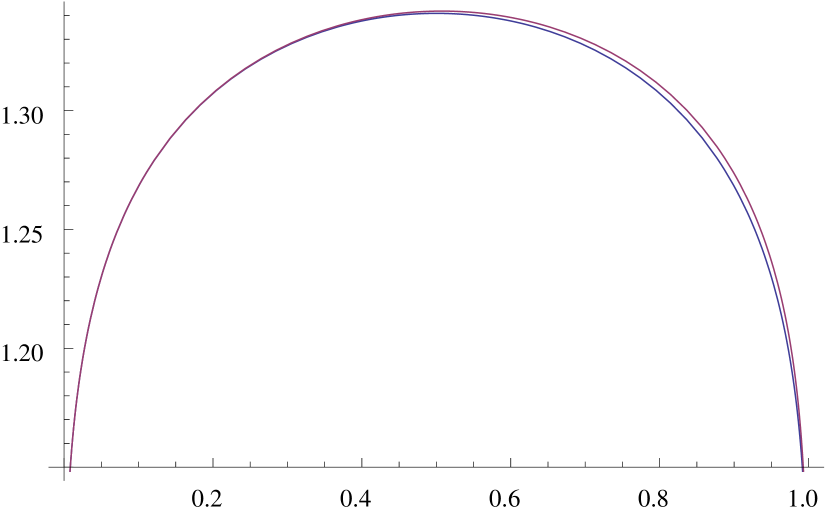
Figure 1: $\mathcal{F}_{2}(x)$ for the Ising model. The blue line is the exact result obtained in [17] and the red one comes from the equation (31).

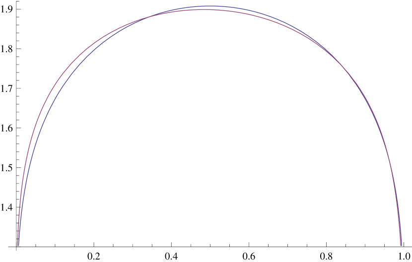
Figure 2: $\mathcal{F}_{3}(x)$ for the Ising model. The blue line is the exact result obtained in [24] and the red one comes from the equation (31).

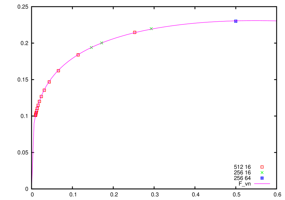
Figure 3: The function $\mathcal{F}_{VN}(x)$ for the Ising model as a function of the cross-ratio $x$. The solid line is the plot of Eq. (2.4), while the data are taken form Ref. [17]. The two integers in the legend are respectively the size $L$ of the system and the size of the interval $\ell$ in units of lattice spacing.

2.3 Rényi entropy

In this subsection by using the results of the last two subsections we give an approximate formula for the Rényi entropy. Using the formula (14) with $\tilde{c}=nc$ and $\delta=\frac{nc}{6}(1-\frac{1}{n^{2}})$ one can write the following formula

$$\mathcal{F}_{n}(x)\sim\frac{1}{(\theta_{3}(\tau))^{1+\frac{nc}{3}-\frac{4c}{3n}}}\left(\frac{x(1-x)}{16q}\right)^{\frac{nc-1}{12}}\sum_{l}C^{2}_{l}(16q)^{2\Delta_{l}}+...,$$ (30)

where we take $\mathcal{F}_{34}^{12}=\mathcal{F}_{n}$. Since the above series is converging very fast, one can just take $H(\tilde{c},\Delta_{l},\Delta_{i},q)\approx 1$ and also consider just the contribution of the field with the minimal conformal weight $\Delta_{min}$, then

$$\mathcal{F}_{n}(x)\sim\frac{1}{(\theta_{3}(\tau))^{1+\frac{nc}{3}-\frac{4c}{3n}}}\left(\frac{x(1-x)}{16q}\right)^{\frac{nc-1}{12}}\Big{(}1+s_{2}(n)\left(\frac{4q}{n^{2}}\right)^{2\Delta_{min}}+...\Big{)},$$ (31)

where we put $s_{2}(n)\equiv s_{2}(n,2\Delta_{min})$. Notice that $\Delta_{min}$ in the above formula is two times bigger than the minimum conformal weight in the minimal models in (26). To see how good is our approximation we discuss Ising model as the simplest unitary minimal model.

For Ising model and $n=2$ the fusion rule is

$$\mathcal{T}_{2}(z_{1},\bar{z}_{1})\bar{\mathcal{T}}_{2}(z_{2},\bar{z}_{2})=1+\sigma^{1}\sigma^{2}+\epsilon^{1}\epsilon^{2};$$ (32)

where $\epsilon^{i}$ and $\sigma^{i}$ are the energy and spin operators of the $i$th copy respectively. In this case $\Delta_{min}=\frac{1}{8}$ is the conformal weight of the two copies of the spin operator. In Fig. 1 we compare the equation (31) with the exact result derived in [17]. The excellent agreement is not a special feature of the critical Ising model. Actually we will verify in section 3, where we describe the exact form of $\mathcal{F}_{2}(x)$, that Eq.(30) for $n=2$ is an excellent approximation for any conformal model.

For $n=3$ part of the fusion rule is

$$\mathcal{T}_{3}(z_{1},\bar{z}_{1})\bar{\mathcal{T}}_{3}(z_{2},\bar{z}_{2})=1+(\sigma^{1}\sigma^{2}+perm)+(\epsilon^{1}\epsilon^{2}+perm)+(\sigma^{1}\sigma^{2}\epsilon^{3}+perm)+...,$$ (33)

where ”$perm$” means that we need to consider all the permutations of the three indices $i=1,2,3$. The dots consider the primary operators that can appear by combining the descendants of different copies of the primary operators [31]. Since the conformal weight of the operator $\sigma^{i}\sigma^{j}\epsilon^{k}$ is quite bigger than the conformal weight of the operator $\sigma^{i}\sigma^{j}$ we do expect that the dominant term be still the contribution of $\sigma^{i}\sigma^{j}$. In Fig 2 we compare the result coming from the equation (31) with the exact result obtained in [24]. Although we ignored many contributions, the result is still satisfactory. In principle the result should be better for small $x$’s than the large ones, however, for unknown reason our formula works better for large $x$’s. It is worth mentioning that if one wants to calculate the next terms just considering the terms like $\sigma^{1}\sigma^{2}\epsilon^{3}$ is not enough. The reason is that the higher order terms in the expansion of $H(\tilde{c},\Delta_{l},\Delta_{i},q)$ for two copies of a primary field could have equal or bigger contribution. Although this is not the case for the Ising model, it simply shows how much it could be complicated to go to the higher levels and keep the calculations consistent. For future use we also give the first few terms of the result for $n>3$. In this case the most dominant term after the contribution of the two spin operators is the contribution of four spin operators with the conformal weight $\frac{1}{4}$. Since the power of $q$ in this case in equation (30) is one half, one expects an important contribution from this term. One can write

$$\mathcal{F}_{n}(x)\sim\frac{1}{(\theta_{3}(\tau))^{1+\frac{n}{6}-\frac{2}{3n}}}\left(\frac{x(1-x)}{16q}\right)^{\frac{n-2}{24}}\Big{(}1+s_{2}(n)\left(\frac{4q}{n^{2}}\right)^{\frac{1}{4}}+s_{4}(n)\left(\frac{4q}{n^{2}}\right)^{\frac{1}{2}}+...\Big{)},$$ (34)

where $s_{4}(n)\equiv s_{4}(n,2\Delta_{min})$ is calculated in [24] and has the following form

$$s_{4}(n,\alpha)=\frac{n}{4}\sum_{{}_{1\leq j_{2}<j_{3}<j_{4}\leq n-1}}\left(\frac{\sin(\pi j_{42}/n)\sin(\pi j_{31}/n)}{\sin(\pi j_{21}/n)\sin(\pi j_{43}/n)\sin(\pi j_{41}/n)\sin(\pi j_{32}/n)}\right)^{2\alpha},$$ (35)

where $j_{kl}=j_{k}-j_{l}$ and $j_{1}=1$. Some properties of $s_{2}(n,\alpha)$ and $s_{4}(n,\alpha)$ are discussed in the Appendix.

2.4 Von Neumann entropy

Since the equations (31) and (34) are simple functions of the number of replicas $n$ one can simply calculate the von Neumann entanglement entropy by just differentiating them with respect to $n$ and evaluating them at $n=1$. Then for Ising model we have

$$\frac{d\mathcal{F}_{n}(x)}{dn}|_{n=1}\sim\theta_{3}^{\frac{-1}{2}}(q)\left(\frac{x(1-x)}{16q}\right)^{\frac{-1}{24}}\Big{(}-\frac{5}{6}\log\theta_{3}(q)+\frac{1}{48}\log\left(\frac{x(1-x)}{16q}\right)+$$

$$s^{\prime}_{2}(1)\left(4q\right)^{\frac{1}{4}}+s^{\prime}_{4}(1)\left(4q\right)^{\frac{1}{2}}\Big{)}+...,\hskip 85.35826pt,$$ (36)

where $s^{\prime}_{2}(1)$ is known from the work in [24] and for generic conformal weight has the following form

$$s^{\prime}_{2}[1,2\Delta_{min}]=+\frac{\sqrt{\pi}\Gamma(1+2\Delta_{min})}{4\Gamma(2\Delta_{min}+\frac{3}{2})}.$$ (37)

Calculation of $s^{\prime}_{4}(1,\frac{1}{4})$ is a very difficult task, we find an approximate value for this quantity by using a numerical method described in the Appendix which yields $s^{\prime}_{4}(1)\simeq 0.126(3)$.

We compare Eq.(2.4) with the numerical data of Ref. [17], based on a tree tensor network algorithm (TTN) [32] applied to a critical one dimensional quantum spin chain in transverse field, corresponding to the CFT minimal model with $c=\frac{1}{2}$. This algorithm gives the full spectrum of the reduced density matrix $\rho_{A}$. From this the moments ${\rm tr}\,\rho_{A}^{n}$ and the entanglement entropy $S_{A}$ are easily evaluated. The data of [17] are taken for a periodic system of length $L$ with a subsystem $A=[v_{1}-u_{1}]\cup[v_{2}-u_{2}]$ composed of two disjoint intervals of identical length $\ell=v_{1}-u_{2}=v_{2}-u_{2}$ at distance $r$. The cross-ratio $x$ is given by

$$x=\left(\frac{\sin\pi\ell/L}{\sin\pi(\ell+r)/L}\right)^{2}.$$ (38)

The ratio $\rho_{A}^{n}/\rho_{\ell}^{2n}$ eliminates the non universal constant $c_{n}$ of Eq. (9) and allows to evaluate, up to obvious factors, the universal function $\mathcal{F}_{n}(x)$ and its contribution $F_{VN}=\partial_{n}\mathcal{F}_{n}(x)|_{n=1}$ to the von Neumann entropy. In Fig. 3 we plot the function $\mathcal{F}_{VN}(x)$ as well as the TTN numerical data, finding a perfect agreement. It is interesting to note that if we use the quantity $s^{\prime}_{4}[1,\frac{1}{4}]$ as a free parameter to fit these data we find a value which is consistent, within the errors, with the value estimated in the Appendix in a completely different context.

3 The special case of two replicas

The case $n=2$ is very interesting and instructive. First, note that Eq. (30) simplifies dramatically because the structure constants become simply

$$C^{2}_{l=rt}=\left(\frac{1}{16}\right)^{4\Delta_{rt}}~{},$$ (39)

thus

$$\mathcal{F}_{2}(x)\sim\frac{1}{\theta_{3}(\tau)}\left(\frac{x(1-x)}{16q}\right)^{\frac{c}{6}-\frac{1}{12}}\sum_{l}q^{2\Delta_{l}}+....$$ (40)

Moreover in this case the four-point function of the twist fields is directly related to the formulation of the CFT on a two-sheeted Riemann surface with two cuts. This is conformally equivalent to a torus whose modular parameter $\tau$ is related to the position of the branch points by Eq.(17). As a consequence it is expected that the torus partition function $Z(\tau)$ of the CFT should show up as a factor of $\mathcal{F}_{2}$ [33, 30, 17].

In this section we would like to reconstruct this relationship within our approach by presenting evidence that a factor of Eq. (40) is just a truncated expansion of the partition function $Z(\tau)$. To this aim, we resort to the following useful formulas

$$\left[x(1-x)\right]^{\frac{1}{12}}=\frac{\left(\theta_{2}(\tau)\theta_{3}(\tau)\theta_{4}(\tau)\right)^{\frac{1}{3}}}{\theta_{3}(\tau)}~{},~{}~{}\theta_{2}(\tau)\theta_{3}(\tau)\theta_{4}(\tau)=2\eta(\tau)^{3}.$$ (41)

The Jacobi theta functions $\theta_{2}(\tau)$ and $\theta_{3}(\tau)$ have been already defined in (17) and similarly we have $\theta_{4}(\tau)=\sum_{n\in\mathbf{Z}}(-1)^{n}q^{n^{2}}$; $\eta(\tau)$ is the Dedekind eta function, defined as

$$\eta(\tau)=q^{\frac{1}{12}}\prod_{n=1}^{\infty}(1-q^{2n})~{};~{}~{}q=e^{i\pi\tau}\,.$$ (42)

These relations, once inserted in Eq. (40), yield

$$\mathcal{F}_{2}(x)\sim\left[\frac{x(1-x)}{16}\right]^{\frac{c}{6}}\sum_{r\,t}|e^{i2\pi\tau(\Delta_{r\,t}-c/24)}|^{2}$$ (43)

where we restored the notation of Eq. (26) and the sum is made over the entries of the Kac table of a given minimal model. One recognizes at once that such a sum is just the truncation of the first few terms of the partition function

$$Z(\tau)=\sum_{r\,t}|e^{2i\pi\tau(\Delta_{r\,t}-c/24)}|^{2}+{\rm higher~{}order~{}terms},$$ (44)

thus one is led to conjecture that the exact form of $\mathcal{F}_{2}(x)$ is simply

$$\mathcal{F}_{2}(x)=\left[\frac{x(1-x)}{16}\right]^{\frac{c}{6}}Z(\tau)\equiv\left|\frac{\eta(\tau)}{\theta_{3}(\tau)}\right|^{2c}Z(\tau)$$ (45)

Actually this formula coincides for $c=1$ with the exact result for compactified boson found long time ago [34, 28, 33] and for $c=\frac{1}{2}$ with the exact result of the critical Ising model obtained in [17].

4 Conclusion

In this paper we found approximate formula (31) for the Rényi entropy ( with arbitrary $n$) of two disjoint intervals of generic minimal conformal field theory. The idea was based on using the elliptic expansion of the conformal blocks appearing in the four point function of the twist fields. Since our formula had a simple relation with $n$, the number of replicas, we were able to do the analytical continuation $n\rightarrow 1$ easily and found the von Neumann entanglement entropy. The von Neumann entropy of two disjoint intervals in the Ising model was investigated as a benchmark and we found excellent agreement between our formula (2.4) and the available numerical results.

Using the perturbative expansion of the four point function of the twist fields in the $n=2$ case we were also able to find a new way to connect explicitly the four point function of the twist fields to the partition function of the conformal field theory on the torus.

Although our perturbative results give rather accurate formulas, even by taking just the first term of the expansion, for the Rényi entropy and von Neumann entropy, it is still tempting to understand how the results can be improved by going to the higher levels. In particular, calculating the von Neumann entropy of more complicated minimal models and checking the results with numerical calculations can shed some light on the possible generalization of our results. Since going to the higher levels of the perturbation is possible just by calculating the structure constants appearing in the OPE of two twist fields - which is itself related to the $k$ point functions of the primary operators - we are faced with the old, unsolved problem of conformal field theory of calculating correlation functions for arbitrary number of fields.

Acknowledgments

FG would like to thank Pasquale Calabrese and Luca Tagliacozzo for fruitful correspondence. MAR thanks John Cardy for many fruitful discussions and comments.

Appendix A The functions $s_{2}(n,\alpha)$ and $s_{4}(n,\alpha)$

In this appendix we deal with the functions $s_{2}(n,\alpha)$ and $s_{4}(n,\alpha)$, where $\alpha$ is related with the conformal weight by $\Delta=\alpha/4$.

The function $s_{2}(n,\alpha)$ has a simple zero at $n=1$ while $s_{4}(n,\alpha)$ has simple zeros at $n=1,2,3$. For integer $n$ both functions have moreover a factor $n$ produced by the translation invariance on the sum of the indices $j_{i}$ so we may assume that both functions have also a zero at $n=0$. This is in particular true for $s_{2}[n,k]$ for integral $k$, where it has been shown in two different contexts and two different ways [35, 30] that $s_{2}[n,k]$ is a polynomial of degree $2k$. The first few polynomials of this set are

$$s_{2}(n,1)=\frac{n}{2}\sum_{j=1}^{n-1}\frac{1}{\sin^{2}\frac{\pi j}{n}}=n\left(\frac{n^{2}}{6}-\frac{1}{6}\right),$$ (A.1)

(this expression has also been found in [14])

$$s_{2}(n,2)=\frac{n}{2}\sum_{j=1}^{n-1}\frac{1}{\sin^{4}\frac{\pi j}{n}}=n\left(\frac{n^{4}}{90}+\frac{n^{2}}{9}-\frac{11}{90}\right),$$ (A.2)

$$s_{2}(n,3)=\frac{n}{2}\sum_{j=1}^{n-1}\frac{1}{\sin^{6}\frac{\pi j}{n}}=n\left(\frac{n^{6}}{945}+\frac{n^{4}}{90}+\frac{4\,n^{2}}{45}-\frac{191}{1890}\right),$$ (A.3)

$$s_{2}(n,4)=\frac{n}{2}\sum_{j=1}^{n-1}\frac{1}{\sin^{8}\frac{\pi j}{n}}=n\left(\frac{n^{8}}{9450}+\frac{4\,n^{6}}{2835}+\frac{7\,n^{4}}{675}+\frac{8\,n^{2}}{105}-\frac{2497}{28350}\right)~{}.$$ (A.4)

It is easy to verify in these cases the general formula of Ref. [24]

$$s_{2}^{\prime}(n,\alpha)_{n=1}=\frac{\sqrt{\pi}\,\Gamma(1+\alpha)}{4\,\Gamma(\frac{3}{2}+\alpha)}=\frac{1}{4}\,B\left(\frac{1}{2},1+\alpha\right),$$ (A.5)

where $B(x,y)$ is the Euler Beta function. In particular, the contribution of the operator energy in critical Ising model is $s_{2}^{\prime}(n,2)_{n=1}=\frac{4}{15}$ and one could add this term to Eq.(2.4) to further improve the formula for the von Neumann entropy.

Assuming that $s_{2}(z,\alpha)$ and $s_{4}(z,\alpha)$ are analytic functions on the complex plane $z$, they admit the following power expansions

$$s_{2}(z,\alpha)=z(z-1)\left(c_{0}+c_{1}z+c_{2}z^{2}+c_{3}z^{3}+\dots\right),$$ (A.6)

$$s_{4}(z,\alpha)=z(z-1)(z-2)(z-3)\left(d_{0}+d_{1}z+d_{2}z^{2}+d_{3}z^{3}+\dots\right).$$ (A.7)

If the two series expansions in the last parenthesis are rapidly convergent series we have, approximately,

$$s_{2}^{\prime}(1,\alpha)\simeq c_{0}+c_{1}+c_{2}+c_{3},$$ (A.8)

and similarly

$$s_{4}^{\prime}(1,\alpha)\simeq 2\left(d_{0}+d_{1}+d_{2}+d_{3}\right)~{}.$$ (A.9)

We fitted $c_{0},c_{1},c_{2},c_{3}$ using the exactly calculable data for $s_{2}(n,\frac{1}{4})$ for integer $n=2,3,\dots 20$ and similarly $d_{0},d_{1},d_{2},d_{3}$; $s_{4}(n,\frac{1}{4})$ for integer $n=4,5,\dots 20$ and verified in both cases that the coefficients $c_{i}$ and $d_{i}$ are rapidly decreasing. In this way $s_{2}^{\prime}(1,\frac{1}{4})$ turns out to be compatible with the exact value. In the same way we estimated

$$s_{4}^{\prime}(1,\frac{1}{4})\simeq 0.126(3)~{},$$ (A.10)

which is the value we put in Eq. (2.4); it turns out to fit nicely the numerical data as shown in Fig. 3. Using the fitted parameters $c_{i}$ and $d_{i}$ one could also study the analytic continuation of $\mathcal{F}_{n}(x)$ to $\mathcal{F}_{z}(x)$, where $z$ is the complex plane of replicas [36] simply by inserting the two functions (A.6) and (A.7) in Eq. (31).

References

- [1] C. G . Callan and F. Wilczek, Phys. Lett. B 333(1994) 55.
- [2] C. Holzhey, F. Larsen, F. Wilczek Nucl.Phys. B424 (1994) 443.
- [3] G. Vidal, J. I. Latorre, E. Rico, A. Kitaev, Phys. Rev. Lett. 90 (2003) 227902 ; J. I. Latorre, E. Rico, G. Vidal, Quant. Inf. and Comp. 4 (2004)48.
- [4] B.-Q.Jin and V.E. Korepin, J. Stat. Phys. 116 (2004) 79.
- [5] H. Casini, M. Huerta, Phys.Lett. B 600 (2004) 142.
- [6] P. Calabrese and J. Cardy, J.Stat.Mech. 0406 (2004) P002.
- [7] S. Ryu and T. Takayanagi, Phys. Rev. Lett. 96 (2006) 181602; S. Ryu, T. Takayanagi, JHEP 0608 (2006) 045.
- [8] M. -C. Chung and I. Peschel, Phys. Rev. B 62 (2000) 4191.
- [9] V. G. Knizhnik, Comm. Math. Phys. 112 (1987) 567.
- [10] J.L. Cardy, O.A. Castro-Alvaredo, B. Doyon, J. Stat. Phys. 130 (2007) 129.
- [11] A. A. Belavin, A. M. Polyakov, A. B. Zamolodchikov Nucl. Phys. B 241 (1984) 333.
- [12] M. Caraglio and F. Gliozzi, JHEP, 0811 (2008 )076.
- [13] S. Furukawa, V. Pasquier and J. Shiraishi, Phys. Rev. Lett. 102 (2009) 170602.
- [14] P. Calabrese, J. Cardy, E. Tonni, J. Stat. Mech. 0911 (2009) P11001.
- [15] , H.Casini and M. Huerta, JHEP 0903(2009) 048.
- [16] P. Facchi, G. Florio, C.Invernizi and S. Pascazio, Phys. Rev. A 78 (2008) 052302.
- [17] V. Alba, L. Tagliacozzo, P. Calabrese, Phys. Rev. B 81 (2010) 060411 (R).
- [18] V. Alba, L. Tagliacozzo and P. Calabrese, J.Stat.Mech. 1106 (2011) P06012.
- [19] F. Igloi and I. Peschel, EPL 89 (2010) 40001.
- [20] M. Fagotti and P. Calabrese, J. Stat. Mech.1004 (2010) P04016.
- [21] P. Calabrese, J. Stat. Mech. (2010) P09013.
- [22] B.-Q. Jin and V. E. Korepin, [ArXiv:1104.1004].
- [23] M. Fagotti, [arXiv:1110.3770].
- [24] P. Calabrese, J. Cardy, E. Tonni, J. Stat. Mech. 1101 (2011) P01021.
- [25] Al. B. Zamolodchikov, Commun. Math. Phys, 96 (1984) 419.
- [26] Al. B. Zamolodchikov, Zh. Eksp. Teor. Fiz., 90 (1986) 1808.
- [27] Al. B. Zamolodchikov, Theor. Math. Phys., 73 (1987) 1088.
- [28] L. Dixon , D. Friedan, E. Martinec, S. Shenker, Nucl. Phys. B 282 (1987) 13.
- [29] C. Crnkovic, G. M. Sotkov, and M. Stanishkov, Phys. Lett. B 220 (1989) 397.
- [30] M. Headrick, Phys. Rev. D 82 (2010) 126010.
- [31] We thank John Cardy for pointing this issue to us.
- [32] M. Fannes, B. Nachtergaele and R. F. Werner J. Stat. Phys. 66 (1992) 939 ; L. Taglacozzo, G. Evenbly, G. Vidal, Phys. Rev. B 80 (2009) 235127.
- [33] O.Lunin and S.D. Mathur, Comm. Math. Phys. 219 (2001) 399.
- [34] Al. B. Zamolodchikov, Sov. Phys. JETP 63(1986) 10161; Nucl. Phys. B 285 (1987) 481.
- [35] M. Billo and A. D’Adda, Int. J. Mod. Phys. A 12 (1997) 2741.
- [36] F. Gliozzi and L. Tagliacozzo, J. Stat. Mech. 1001 (2010) P01002.