Information dynamics algorithm for detecting communities in networks
Abstract
The problem of community detection is relevant in many scientific disciplines, from social science to statistical physics. Given the impact of community detection in many areas, such as psychology and social sciences, we have addressed the issue of modifying existing well performing algorithms by incorporating elements of the domain application fields, i.e. domain-inspired. We have focused on a psychology and social network - inspired approach which may be useful for further strengthening the link between social network studies and mathematics of community detection. Here we introduce a community-detection algorithm derived from the van Dongen’s Markov Cluster algorithm (MCL) method [5] by considering networks’ nodes as agents capable to take decisions. In this framework we have introduced a memory factor to mimic a typical human behavior such as the oblivion effect. The method is based on information diffusion and it includes a non-linear processing phase. We test our method on two classical community benchmark and on computer generated networks with known community structure. Our approach has three important features: the capacity of detecting overlapping communities, the capability of identifying communities from an individual point of view and the fine tuning the community detectability with respect to prior knowledge of the data. Finally we discuss how to use a Shannon entropy measure for parameter estimation in complex networks.
1 Introduction
Detecting communities is a task of great importance in many disciplines, namely sociology, biology and computer science [22, 18, 6, 20, 1], where systems are often represented as graphs. Community detection is also linked to clustering of data: many clustering methods establish links among representative points that are nearer than a given threshold, and then proceed in identifying communities on the resulting graphs [3, 2]. Given a graph, in a broad sense, a community is a group of vertices “more linked” than between the group and the rest of the graph. This is clearly a poor definition, and indeed, on a connected graph, there is not a clear distinction between a community and the rest of the graph. In general, there is a continuum of nested communities whose boundaries are somewhat arbitrary: the structure of communities can be seen as a hierarchical dendogram [15].
In general, community detection algorithms rely on global quantities like betweenness, centrality, etc. [15, 14] and most algorithms require the graph to be completely known. This constraint is problematic for networks like the World Wide Web, which for all practical purposes is too large and too dynamic to ever be fully known.
Moreover in complex networks, and in particular in social networks, it is very difficult to give a clear definition of community: it is caused by the fact that nodes often results in overlapping communities because they belong to more than one cluster or module or community. The problem of overlapping communities was discussed in [17] and recently a solution to it were presented in [11]. For instance people usually belong to different communities at the same time, depending on their families, friends, colleagues, etc.: so each people, making a subjective community detection algorithm, has its own vision of communities in his social environment.
In social networks, the definition of a community could be linked to the human capability of information processing, particularly the poor evaluation of probabilities. When faced with insufficient data or insufficient time for a rational processing, we humans have developed algorithms, denoted heuristics, that allows to take decisions in these situations. The modern approach to the study of cognitive heuristics defines them as those strategies that prevent one from finding out or discovering correct answers to problems that are assumed to be in the domain of probability theory. The ratio of a cognitive algorithm for community detection is based on the fact that humans’ networks are the results of the individual stategies of single subjects; on the other hand they are presumably shaped and evolved by the social structures in which they live [10, 9].
The paper is organized as follows: we start by describing a new algorithm for detecting communities in complex networks in Section 2. Considering psychological notions as mentioned above, we adopted local algorithm where an individual is simply modeled as a memory and a set of connections to other individuals. The “learning” (nonlinear) phase is modeled after competition in chemical/ecological world, where resources fighting each other in order not to fall into oblivion. In Section 3 we describe the first algorithm in which information about neighboring nodes is propagated and elaborated locally, but the connections do not change. Here we want to emphasize not only the good efficiency of the algorithm in detecting community but also its capability to discover overlapping nodes and a sort of subjective vision of hierarchical levels of the network. Next, in Section 4 we give an interpretation of Shannon entropy of information as quality function for estimating models parameters. Finally we discuss our results and we propose future steps in Conclusions.
2 Competion process
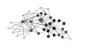
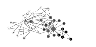
We consider individuals, labeled from to . Let us denote by the adjacency matrix, (0) indicates the presence (absence) of a link from site to site ; all links have the same weight (Figure 1). Each individual is characterized by a state vector , representing his knowledge of the outer world. We interpret as a probability distribution, assuming that is the probability that individual belongs to the community . Thus, is normalized on the index . We shall denote by the state of the all network at time , with . We shall initialize the system by setting , where is the Kroneker delta, if and zero otherwise. In other words, at time 0 each node only knows about itself.

As mentioned the competition phase is modeled thinking to a chemical/ecological analogy. Our algorithms are based on the concept of diffusion and competitive interaction in network structure introduced by Nicosia et al. [16].
If two populations and are in competition for a given resource, their total abundance is limited [13]. After normalization, we can assume , i.e., and are the frequency of the two species, and . The reproductive step is given by , which we assume to be represented by a power . For instance, models the birth of individuals of a new generation after binary encounters of individuals belonging to the old generation, with noneverlapping generations (eggs laying) [4].
After normalization we obtain:
| (1) |
Introducing (), we get the map
| (2) |
whose fixed points (for ) are 0 and (stable attractors) and (unstable), which separates the basins of the two attractors. Thus, the initial value of , , determines the asymptotic value, for , , and for , .
By extending to a larger number of components for a probability distribution , the competition dynamics becomes
| (3) |
and the iteration of this mapping, for , leads to a Kroneker delta, corresponding to the larger component. However, the alternation between information and competition can generate interesting behaviors.
3 Information Dynamics Algorithm
The dynamics of the network is given by an alternation of communication and elaboration phases. Communication is implemented as a simple diffusion process, with memory . The memory parameter allows us to introduce some limitations in human cognition such as the mechanism of oblivion and the timing effects: the most recent information has more relevance than the previous one [21, 7].
We assume that each individual spends the same amount of time in communication, so that people with more connections dedicate less time to each of them. Since the amount of available time is limited, we normalize the adjacency matrix on the columns (i.e., we assign at each link the inverse of the output degree of the incoming node), forming a Markov matrix
| (4) |
Note that in many mathematical texts the indices are inverted, so that the Markov matrices are normalized on the rows. We prefer the “physics” notation so that matrix multiplication with a probability distribution takes the usual form . Then in the communication phase, the state of the system evolves as
| (5) |
As described in the Eq. 3, the competition phase is modeled thinking to a competive interaction between the nodes in the network [16].
In this way the dynamic of the model is given by a sequence :
| (6) |
We assume that individuals’ memory is large enough so that they can keep track of all information about all other individuals. In a real case, one should limit this memory and apply an input/output filtering. Individuals do not change their connectivity. For testing purposes we use three networks and analyzing and discussing our model peculiarities. The three case studies, of growing or different complexity, are: a simple artificial network used to show the typical output of our algorithm, the Zachary karate club network [23] and the bottlenose dolphins network [12].
3.1 Simple artificial network
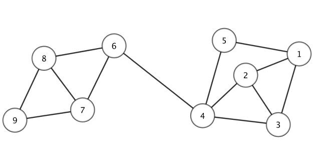
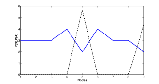
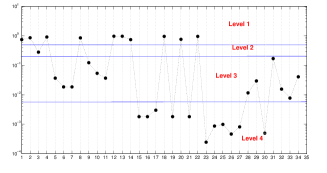
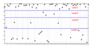
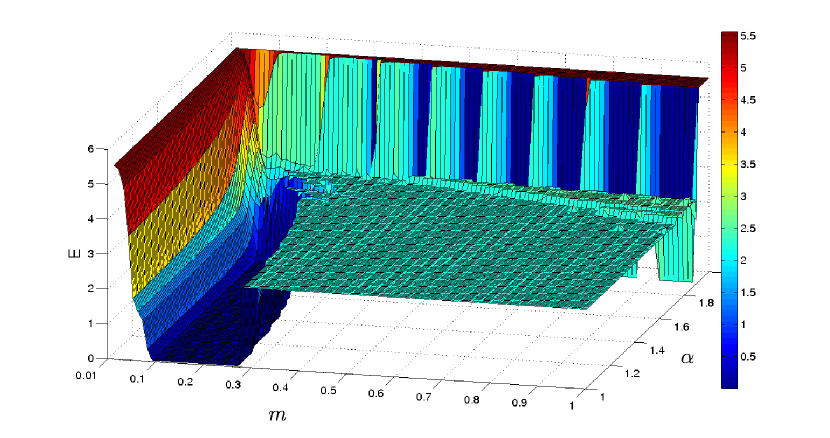
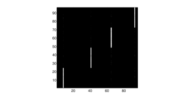
In this first case study the algorithm face with a very simple task and converges to an optimal solution in few iterations and for a wide range of model’s parameters and . Analyzing state matrix S(t), it is possible to identify two different communities marked by nodes 5 and 9.
S(T)=
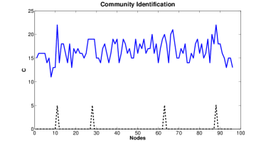
In Figure 3(b) it is possible to identify two different communties highlighted by upper values in the graph. The first community is composed by node 1-2-3-4-5 and the second one by 6-7-8-9. Our algorithm is capable also to detect overlapping nodes (4 and 6) as ”middle” values between blue lines. In this way each node knows exactly its role in the network.
3.2 Zachary ”Karate Club”
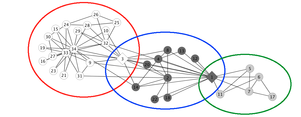
The second test case is a typical network literature example: the network proposed by Zachary in the 1977 , and known as ”karate club” [23]. Although this network (Figure 4(a)) is rather small, our algorithm shows interesting results. With and the algorithm has detected three communities in few steps as described in the Figure 4(b).
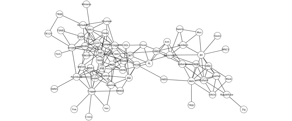
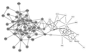
3.3 Bottlenose dolphin Network
The third case study concerns a community network of dolphins. The network we study was constructed from observations of a community of 62 bottlenose dolphins over a period of seven years from 1994 to 2001 [12].


4 Entropy of information
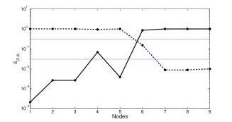
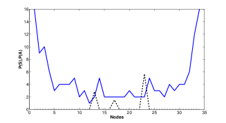
In order to present the temporal results in a compact way, we computed the entropy of a configuration , using the cumulative distribution over the non-normalized index,
| (7) |
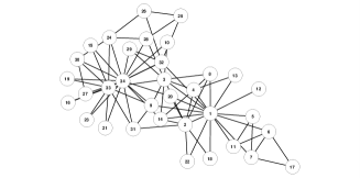
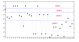
The entropy is maximal for the flat distribution, when each node knows only itself, and minimal (zero) what all the network has only one label (or has become just one star for the rewiring algorithm). If the population is evenly distributed among clusters, the entropy is . Let us to study the artificial complex network illustrated in Figure 1. This network is composed by three levels with different probability to have a link in a region.
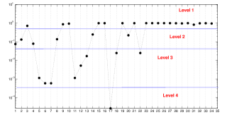
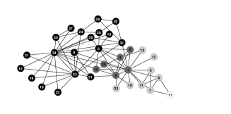
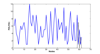
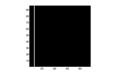
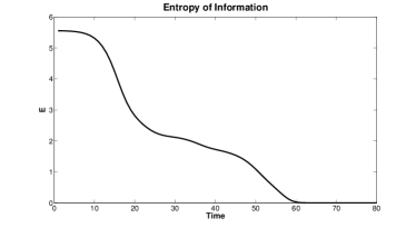
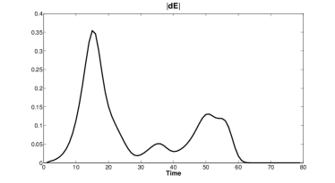
As we observed our algorithm is able to observe all levels of a hierarchical network. In Figure 12(a) it is possible to identify the final level of the artificial network. The value of Entropy can help us understand the structure of the network at priori. In fact, different levels of a hierarchical structure are identified by the plateau as we can observe in Figure 12(b). This result is emphasized by the entropy’s first derivative where we can observe three distinct peaks (Figure 12(c)). The final monocluster, using the adjacency matrix in the Eq. 6, is identified by the major hub in the network (Figure 12(d)).
 |
 |
| (a) | (b) |
 |
 |
| (c) | (d) |
 |
 |
| (a) | (b) |
5 Conclusion
In this paper we have described an algorithm to identify the communities structures in a network from a local point of view.
The method is based on pure information propagation where the nonlinear part of these method, responsible for the actual elaboration of information, is inspired by a chemical/ecological competition model [16].
There is not a unique definition of a community, so an exploratory algorithm, like the one that humans have presumably developed during their evolution, should present different clustering for different values of the parameters, or for different iterations.
In this implementation we adopted a frequency-based approach and an unbounded memory at the level of nodes. Unbounded memory means that the node’s state vector has not been limited and it could potentially reach a size equal to the network size . Despite this because of the explanation and normalization phases are sufficient to avoid this problem. Nevertheless it will be very important to limit the computational resources of the node explicitly, as suggested by Simon in 1955 [19], so increasing both the ecological plausibility of the model and the insights which drive the algorithm design.
The results that we have obtained are promising. The method under investigation is not competitive with respect to others (see the review [8]), but it provides a natural “scanning” of the various clustering levels. Moreover, our method can be naturally applied to weighted graphs. We have demonstrated, through the definition of Entropy of Information, our algorithm is efficient to discover all cluster levels for general networks.
We believe that the local algorithm procedure will not only allow to us to study much larger networks but also to mimic single human behavior in social network trough specific and simple heuristics decision rules. The model parameters and play a crucial role for the detection of communities. These results suggests how cognitive heuristics could be designed as those mechanism which allow humans to optimize those parameters in order to maximize the gathered information from the environment. Following this assumption the future works will investigate what kind of computational procedures could be used to mimic this human behavior. We plan to investigate the consequences of bounded memory and computational resources of nodes, in particular in a dynamic environment.
Acknowledgments
This work is financially supported by Recognition Project: RECOGNITION is a 7th Framework Programme project funded under the FET initiative.
Bibliography
References
- Albert and Barabási [2002] R. Albert and A. L. Barabási. Rev. Mod. Phys., (74):47, 2002.
- Blatt et al. [1996] M. Blatt, S. Wiseman, and E. Domany. Superparamagnetic clustering of data. Phys. Rev. E, (76):3251–3254, 1996.
- Brandes et al. [2006] U. Brandes, D. Delling, M. Gaertler, R. Gorke, M. Hoefer, Z. Nikoloski, and D. Wagner. On finding graph clusterings with maximum modularity. In Proceedings of the 33rd International Workshop on Graph-Theoretical Concepts in Computer Science (WG’07), 2006.
- de Freitas et al. [2000] J. E. de Freitas, L.S. Lucena, L.R. da Silva, and H.J. Hilhorst. Critical behavior of a two-species reaction-diffusion problem. Phys. Rev. E., (61):6330–6336, 2000.
- Dongen [2009] S. Van Dongen. Graph clustering via a discrete uncoupling process. SIAM. J. Matrix Anal. and Appl., (30):121–141, 2009.
- Dorogovtesev and Mendes [2003] S. N. Dorogovtesev and J. F. F. Mendes. Evolution of Networks. Oxford University Press, Oxford, 2003.
- Forster and Davis [1984] K. I. Forster and C. Davis. Repetition priming and frequency attenuation. Journ. Exp. Psyc.: Learning Memory and Cognition, 10(4), 1984.
- Fortunato [2010] Santo Fortunato. Community detection in graphs. Physics Reports, 486(3-5):75 – 174, 2010. ISSN 0370-1573. doi: DOI: 10.1016/j.physrep.2009.11.002.
- Gigerenzer and Gaissmaier [2011] G. Gigerenzer and W. Gaissmaier. Heuristic decision making. Ann. Rev. of Psyc., (62):451–482, 2011.
- Gigerenzer and Goldstein [2002] G. Gigerenzer and G. Goldstein. Models of ecological rationality: The recognition heuristic. Psyc. Rev., 109(1):75–90, 2002.
- Lancichinetti et al. [2009] A. Lancichinetti, S. Fortunato, and J. Kertész. Detecting the overlapping and hierarchical community structure of complex networks. New Journal of Physics, 033015(11), 2009.
- Lusseau et al. [2003] D. Lusseau, K. Schneider, O. J. Boisseau, P. Haase, E. Slooten, and S. M. Dawson. Behavioral Ecology and Sociobiology, (54):396–405, 2003.
- Murray [2002] J.D. Murray. Mathematical biology. Number v. 1 in Interdisciplinary applied mathematics. Springer, 2002. URL http://books.google.it/books?id=aHoaKQEACAAJ.
- Newman [2004] M.E.J. Newman. Detecting community structure in networks. Europ. Phys. J. B, (38):331–330, 2004.
- Newman and Girvan [2004] M.E.J. Newman and M. Girvan. Finding and evaluating community structure in networks. Phys. Rev. E, (69):026113, 2004.
- Nicosia et al. [2011] V. Nicosia, F. Bagnoli, and V. Latora. Impact of network structure on a model of diffusion and competitive interaction. EPL, 94(68009), 2011.
- Palla et al. [2005] G. Palla, I. Derény, and T. Vickset. Nature, 435:814, 2005.
- Scott [2000] J. Scott. Social Networks Analysis: A Handbook. Sage, London, 2nd, edition, 2000.
- Simon [1955] H.A. Simon. A behavioral model of rational choice. The Quarterly Journal of Economics, 69(1):99–118, 1955.
- Strogatz [2001] S.H. Strogatz. Nature(London), (410):268, 2001.
- Tulving et al. [1982] E. Tulving, D. L. Schacter, and H. A. Stark. Priming effects in word fragment completion are independent of recognition memory. Journ. Exp. Psyc.: Learning Memory and Cognition, 8(4), 1982.
- Wasserman and Faust [1994] S. Wasserman and K. Faust. Social Networks Analysis. University Press, Cambridge, England, 1994.
- Zachary [1977] W. W. Zachary. An information flow model for conflict and fission in small groups. Journal of Anthropological Research, (33):452–473, 1977.