HU-EP-11/56
SFB/CPP-11-74
Numerical evaluation of one-loop QCD amplitudes

Abstract

We present the publicly available program NGluon allowing the numerical evaluation of primitive amplitudes at one-loop order in massless QCD. The program allows the computation of one-loop amplitudes for an arbitrary number of gluons. The focus of the present article is the extension to one-loop amplitudes including an arbitrary number of massless quark pairs. We discuss in detail the algorithmic differences to the pure gluonic case and present cross checks to validate our implementation. The numerical accuracy is investigated in detail.

1 Introduction

The automation of next-to-leading (NLO) corrections to multi-particle processes in the Standard Model is an important step in making precision predictions for signal and background reactions studied at the Large Hadron Collider (LHC) at CERN. Recent years have seen considerable progress in simplifying this complex task into a definite algorithm for arbitrary processes [1, 2, 3, 4]. Full NLO distributions for a growing number of $2\rightarrow 4$ [5, 6, 7, 8, 9, 10, 11, 12] and even $2\rightarrow 5$ [13, 14, 15] processes have now been achieved. The degree of automation to which the virtual corrections to NLO observables can be computed has steadily improved [16, 17, 18, 19, 20, 21, 22, 23].

In this article we review the computations of multi-parton amplitudes in massless QCD using the NGluon c++ library [24]. The algorithm employs the generalised unitarity cutting procedure to construct one-loop amplitudes from on-shell tree-level building blocks which we review in Section 2. We then describe the inclusion of amplitudes with multiple fermion pairs in Section 3 and present a detailed analysis of the performance and validity of our approach in Section 4. We finish by presenting our conclusions in Section 5.

2 Review of Generalised Unitarity

The method of generalised unitarity has been studied extensively over the last few years. Based on a purely algebraic approach, the method can be used to formulate a numerical algorithm for the computation of one-loop amplitudes [26, 25, 4]. Detailed and helpful reviews on the subject can be found in references [27, 28, 29].

The one-loop amplitudes we consider in this article are colour ordered QCD primitive amplitudes where both colour generators and internal colour flow structure have been stripped off leaving the simplest gauge invariant building blocks of the full amplitude. Each of these terms has a well defined ordering of external legs and internal propagators.

A general one-loop primitive amplitude with no external massive particles, regulated in $D=4-2\epsilon$ dimensions, can be expressed in terms of a basis of scalar two-, three- and four-point integral functions together with rational terms [25],

$$A^{(1)}(p_{1},\cdots,p_{n})=\sum_{i<j<k<l}c_{4;i,j,k,l}I_{4}(s_{i,k-1},s_{j,l-1};s_{i,j-1},s_{j,k-1},s_{k,l-1},s_{l,i-1})$$

$$+\sum_{i<j<k}c_{3;i|k|k}I_{3}(s_{i,j-1},s_{j,k-1},s_{k,i-1})+\sum_{i<j-1}c_{2;i|j}I_{2}(s_{i,j-1})$$

$$-\frac{1}{6}\sum_{i<j<k<l}c_{4;i,j,k,l}^{[4]}-\frac{1}{2}\sum_{i<j<k}c_{3;i,j,k}^{[2]}-\frac{1}{6}\sum_{i<j-1}s_{i,j-1}c_{2;i,j}^{[2]}+\mathcal{O}(\epsilon).$$ (1)

Here $s_{i,j}=(p_{i}+\cdots+p_{j})^{2}$ are the Lorentz invariants of the amplitude. $I_{4},I_{3}$ and $I_{2}$ are the well known scalar integral functions that can be written in terms of logarithms, dilogarithms and the dimensional regulator, $\epsilon$. Thanks to public programs for the numerical evaluation of the scalar integrals for arbitrary kinematics, e.g. FF [30], OneLOop [31] or QCDLoop [32] , the only process dependent quantities are the coefficients $c_{k;X}$.

The box coefficients, $c_{4;X}$, can be extracted by applying maximal cuts to the one-loop primitive amplitude, factorises into a product of four tree-level amplitudes. The lower point integral coefficients are then computed systematically by considering fewer cuts and subtracting the contribution from the higher point functions previously evaluated. In each case the integrand can be parametrised by a polynomial of the scalar products between the loop momentum and spurious vectors that can be neatly described by the van Neerven-Vermaseren basis. The construction in NGluon follows the description of reference [33]. The coefficients of the aforementioned polynomial can be efficiently computed using a discrete Fourier projection.

For the rational terms we need to consider cuts in five, or more, dimensions. In the Four Dimensional Helicity (FDH) scheme this can be achieved using a mass-shifted representation of the amplitude, where the coefficients $c_{4}^{[4]},c_{3}^{[2]}$ and $c_{2}^{[2]}$ can be extracted from a discrete Fourier projection over the additional mass parameter [34]. The mass shifted integrands factorise into tree-level amplitudes with massive scalar particles and massive fermions.

3 Extension to Multiple Fermion

The extension of the pure gluonic case to multiple fermions has basically two fundamental new features:

1. more complicated tree-level amplitudes

2. restrictions when sewing tree-level amplitudes together to reconstruct the integrand

In the pure gluonic case, all tree-level amplitudes that can occur in a unitarity cut can be assigned a unique colour ordering. This means that they can always be computed with the well known Berends-Giele recursion relations [36]. The simple reason for this is the fact that restoring the colour to the primitive amplitude both external legs and loop lines live in the adjoint representation.

With the inclusion of quarks in the fundamental representation, this one-to-one correspondence is in general lost. It happens that through unitarity cuts basic building blocks appear that do not belong to any colour structure which would occur in the computation of a Born amplitude. This can be seen, for instance, at those quark-gluon primitive amplitudes contributing solely to the subleading colour part of the full amplitude. As an example, consider the primitive amplitude $A^{\rm prim}(\overline{Q}_{1};g_{2};Q_{3};g_{4})$ where the fixed ordering of external particles is such that a quark anti-quark pair is separated by one gluon. In certain bubble and triangle cuts, for example, among others, the following building block arises: $A^{\rm tree}(\overline{Q}_{1};g_{\,2};Q_{\,\rm loop};g_{\,\rm loop})$ as illustrated in figure 1. In $A^{\rm tree}(\overline{Q}_{1};g_{\,2};Q_{\,\rm loop};g_{\,\rm loop})$, the non-abelian gluon interactions are missing and in addition, the structure is not colour-ordered. It is possible to compute these building blocks as a linear combination of colour-ordered tree amplitudes. However, in NGluon all tree amplitudes are computed directly with help of colour stripped Feynman rules [35]. One has to specify only the external leg order and its particle content. Tree amplitudes are then evaluated independently on whether they can be assigned a definite colour structure or not.

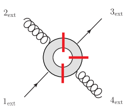
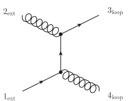
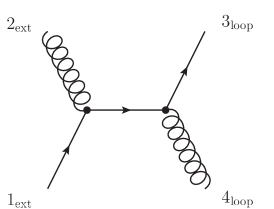
Figure 1: A triple cut of the primitive amplitude $A^{\rm prim}(\overline{Q}_{1};g_{2};Q_{3};g_{4})$ leading to a four point tree amplitude $A^{\rm tree}(\overline{Q}_{1\,{\rm ext}};g_{\,2\,{\rm ext}};Q_{\,3\,{\rm loop}};g_{4\,{\rm loop}})$ consisting of the above two ordered tree diagrams. “ext” resp. “loop” denote external legs, resp. on-shell loop legs. Note the absence of any gluon self interactions.

Technically, we follow for the trees an off-shell bottom-up approach. This means that after the order of $n$ external legs with appropriate particle content has been fixed, one starts computing all one-point currents, i.e. polarisation vectors for gluons and spinors for quarks. Subsequently, higher point currents are computed systematically from lower point currents. The $n$-point amplitude is computed by contracting the $(n-1)$-point current with the $n$th one-point current. This procedure has the advantage that many currents can be reused during the computation. The most complicated vertex, the four gluon vertex, dictates the asymptotic scaling behaviour, which can be shown to be polynomial of order $O(n^{4})$.

In the context of generalised unitarity, an additional reduction in complexity can be achieved: For different topologies, those currents that involve exclusively external legs never change and can be computed once in the beginning for all possible cuts. An amplitude evaluation is then equivalent to joining new currents that involve loop legs with external, already known currents. This procedure reduces the polynomial scaling even further to order $O(n^{3})$ [24].

In the highly symmetric pure gluonic case, every cut is possible. In other words, there is always a loop propagator which connects directly two external legs. This is not necessarily the case if more then one fermion line is involved in the amplitude. Take for example a closed quark loop and one external $\overline{q}q$-pair: The external quark line will never enter the loop and can’t be put on shell.

In order to describe this problem algorithmically, we use the concept of a parent diagram. In our framework, a parent diagram of an $n$-point amplitude is an abstract one-loop diagram with $n$ fictitious three-point vertices and $n$ propagators. The particle content of its propagators labels the possible on-shell settings. In addition, it knows also which propagators do not exist. The propagator content of the parent diagram is therefore the backbone to compute systematically all integral coefficients. The procedure is exactly like in the pure gluonic case with the exception that if a topology involves a non-existing propagator, the topology is simply skipped.

In order to determine the parent diagram, one draws an abstract loop without specifying any particle content yet and attaches all ordered external legs to it. One starts with the specification of the particle content of an arbitrary initial propagator in the loop and determines with the external leg attached to this propagator the content of the next propagator in the loop. This procedure is repeated for the whole diagram until one hits the initial propagator.

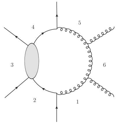
Figure 2: A six-point parent diagram for a primitive with two external fermion lines. The first propagator is initialised with a gluon. The third one is then unphysical and represented by a blob.

One sees immediately that certain propagators of the parent diagram can’t be assigned properly in case we are dealing with either 1) a closed fermion loop plus at least one external fermion line or 2) two (or more) fermion lines where a quark-antiquark pair is separated by another quark-antiquark pair. An example is given in figure 2. Literally speaking, this means the following: under the grey blob in figure 2 live two fermion lines which can’t be represented by a valid QCD propagator. As soon as the enclosed quark line “leaves” the blob, the parent diagram follows the same pattern as before. With the knowledge of the parent diagram and the external legs, the primitive is uniquely determined.

Another subtlety occurs for certain subleading colour contributions where a distinct cut requires a tree consisting of two fermion lines which belong, however, inside the one-loop amplitude to the same fermion line. Formally, such trees must be treated like two different flavour lines since otherwise one would include contributions that belong to amplitudes with a closed fermion loop, a different class of amplitudes. A simple four-point example is given in figure 3.

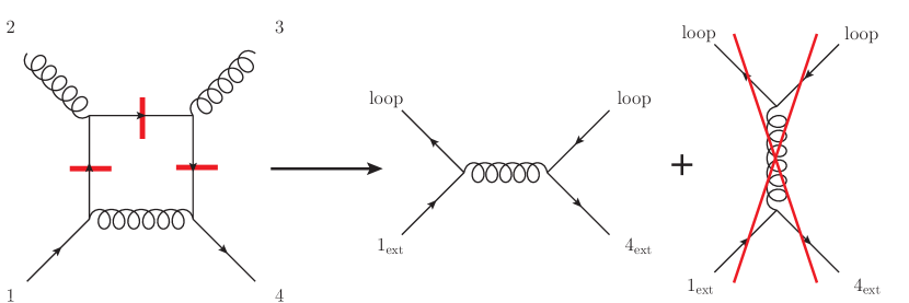
Figure 3: Triple cut with a two fermion tree amplitude. Although at one-loop level, there is only one fermion line, they must be treated at tree-level as two distinct flavours in order to avoid contributions from a closed quark loop (right diagram crossed out).

4 Performance and Cross Checks

The first detailed verification of the implementation comes from comparison with the well known universal Infra-Red and Ultra-Violet poles in the dimensional regulator, $\epsilon$. This analytic cross check tests the four-dimensional (or cut-constructible) parts of the amplitude and can also give some hints as to a loss of numerical precision.

In order to get an overall estimate for the numerical accuracy, we use the following observation: A re-scaling of the external momenta is equivalent to a simple change of units and should therefore be physically equivalent. Since the floating point arithmetic at the hardware level changes, the difference between the two evaluations — rescaled and un-rescaled — can be used to estimate the numerical uncertainty. The validity of this approach is investigated in detail in [24]. This test is very convenient to detect numerical instabilities and has in addition the advantage that it is independent from any analytic input. Of course, it is not at all suited to check the correctness of the implementation itself and has the drawback of a factor of two in the runtime. In case, the internal accuracy checks do fail, the phase space point can be reprocessed using higher precision with the qd package described in reference [39].

Besides the poles, we made cross checks against known analytical and numerical results. For the trivial extension of the pure gluonic case to a closed quark loop with exclusively external gluons, we find full agreement with the reference phase space points in [37]. The correctness of the implementation for primitives with one external quark line has been tested intensively against all formulae of the $\overline{q}qggg$ results given in [35]. The agreement of these 5-point cases holds both for different helicity configurations and quark-antiquark separations. For higher $n$-point functions, we checked the IR-finite amplitudes $A(\overline{q}_{1},g_{2},...,q_{i},...g_{n})$ with helicity configuration $-++...+$ given analytically in [38] for all possible quark-antiquark separations and find numerical agreement. An example for an 8-point function is shown in figure 4. Only a very small fraction of events show an accuracy of less then 3 digits which is enough for most practical calculations. While the accuracy for different quark-antiquark separations does not differ much in the mixed quark-gluon loop, it does for a closed quark loop. This is simply a consequence of the fermion loop primitive amplitudes having fewer allowed propagators as the $\overline{q}q$-separation increases. This is also the reason why the computation time differs by roughly one order of magnitude depending on the separation of the quark and the antiquark. An example for the runtime difference is shown in table 1. Due to the vanishing of massless tadpoles, the largest two separations in the closed quark loop do not contribute.

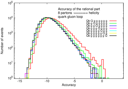
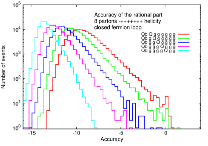
Figure 4: Accuracy distribution for the rational part of $(\overline{q}q+6\,g)$-primitives. The histograms plot the number of events against the decadic logarithm of the relative accuracy (# of valid digits) between the result from NGluon and the analytic formulae in [38] for all possible separations of the two external quark legs.

Table 1: Runtime in milli seconds for primitives with one quark antiquark pair on an Intel(R) Core(TM)2 Duo CPU E8400 @ 3.00GHz processor. While in the mixed quark-gluon loop the runtime increases with larger $\overline{q}q$-separation, the contrary is the case for the closed quark loop.

6-point example:
$\overline{q}q$-separation	0	1	2	3	4
mixed quark-gluon loop	4.85	5.95	7.27	8.77	10.30
closed quark loop	6.13	2.61	0.72	0.01	0.01

8-point example:
$\overline{q}q$-separation	0	1	2	3	4	5	6
mixed quark-gluon loop	19.84	22.08	23.81	27.35	30.54	34.13	38.07
closed quark loop	26.31	14.82	7.57	3.14	0.91	0.03	0.03

For the multiple fermion case, we find agreement in the poles for all primitives that we have tested (up to 5 external quark-antiquark pairs).

When computing the full amplitude out of primitives, many tree-level amplitudes can be reused. The necessary conditions are: 1) the loop momentum for a topology agrees, 2) both loop and external flavours agree and 3) both loop and external helicities agree. It is important to stress that for one primitive with fixed helicity, no information can be reused. The cache system starts first its work when one is dealing with either different permutations of primitive amplitudes or with different helicity amplitudes (if, for example, an average over all helicities is carried out). Take for instance a bubble cut with two trees: flipping one helicity in one tree does not affect the other tree which can be recycled. Similar considerations apply to permutations that affect only trees inside one cut: At any time, the other tree is left untouched and can be reused. Note that we reuse only full tree amplitudes and no off-shell currents. Especially when dealing with permutations, a cache that works on current level could be constructed. The book-keeping for such an approach is however much more involved. As a consequence this possibility is not yet used in NGluon .

We have implemented the cache system via a binary tree which is part of the c++ standard template library. Due to the internal index system, the cache is restricted to 13 external legs with six (different flavour) external quark pairs. The asymptotic behaviour is estimated via the computation time of $(n-1)!/2$ permutations of primitives. For low multiplicity (in our case four point amplitudes), there is an overhead using such a system since the stored amplitudes are usually only three-point or at most four point functions and very quickly evaluated. From five external legs on until eight one gains speed up factors between 2 and 3. For higher multiplicities, however, the amount of storage information is so large that the cache starts to slow down the computation compared to the direct evaluation without cache. It is expected that for the leading colour approximation where far less primitives are needed, the performance of the cache is more efficient.

5 Conclusions

NGluon is a publicly available program to compute primitive amplitudes with a fixed order of external legs in pure gauge theory. We have shown the extension of the program to an arbitrary number of external massless quarks: For a fixed order of helicity and flavour of the external particles, the primitive amplitude is evaluated in a fully automatic way. As internal accuracy check, we find that the “scaling test” gives reliable estimates. We have made several cross checks with known results from the literature and find numerical agreement with our implementation. An additional cache system which recycles tree amplitudes for the unitarity cut can lead to speed up factors between two and three. First phenomenological applications are in preparation.

References

References

- [1] Bern Z, Dixon L, Dunbar D and Kosower D 1994 Nucl. Phys. B 425 217. [hep-ph/9403226].
- [2] Britto R, Cachazo F and Feng B 2005 Nucl. Phys. B 725 275. [hep-th/0412103].
- [3] Ossola G, Papadopoulos C and Pittau R 2007 Nucl. Phys. B 763 147. [hep-ph/0609007].
- [4] Berger C, Bern Z, Dixon L, Febres Cordero F, Forde D, Ita H, Kosower D and Maitre D, 2008 Phys. Rev. D 78 036003. [arXiv:0803.4180 [hep-ph]].
- [5] Berger C, Bern Z, Dixon L, Febres Cordero F, Forde D, Gleisberg T, Ita H, Kosower D and Maitre D 2010 Phys. Rev. D 82 074002. [arXiv:1004.1659 [hep-ph]].
- [6] Berger C, Bern Z, Dixon L, Febres Cordero F, Forde D, Gleisberg T, Ita H, Kosower D and Maitre D 2009 Phys. Rev. D 80 074036. [arXiv:0907.1984 [hep-ph]].
- [7] Berger C, Bern Z, Dixon L, Febres Cordero F, Forde D, Gleisberg T, Ita H, Kosower D and Maitre D 2009 Phys. Rev. Lett. 102 222001. [arXiv:0902.2760 [hep-ph]].
- [8] Greiner N, Guffanti A, Reiter T and Reuter J 2011 Phys. Rev. Lett. 107 102002. [arXiv:1105.3624 [hep-ph]].
- [9] Bevilacqua G, Czakon M, Papadopoulos C and Worek M 2010 Phys. Rev. Lett. 104 162002. [arXiv:1002.4009 [hep-ph]].
- [10] Denner A, Dittmaier S, Kallweit S and Pozzorini S 2011 Phys. Rev. Lett. 106 052001. [arXiv:1012.3975 [hep-ph]].
- [11] Bredenstein A, Denner A, Dittmaier S and Pozzorini S 2009 Phys. Rev. Lett. 103 012002. [arXiv:0905.0110 [hep-ph]].
- [12] Melia T, Melnikov K, Rontsch R and Zanderighi G 2011 Phys. Rev. D 83 114043. [arXiv:1104.2327 [hep-ph]].
- [13] Frederix R, Frixione S, Melnikov K and Zanderighi G 2010 J. High Energy Phys. JHEP1011(2010)050. [arXiv:1008.5313 [hep-ph]].
- [14] Berger C, Bern Z, Dixon L, Febres Cordero F, Forde D, Gleisberg T, Ita H, Kosower D and Maitre D 2011 Phys. Rev. Lett. 106 092001. [arXiv:1009.2338 [hep-ph]].
- [15] Ita H, Bern Z, Dixon L, Cordero F, Kosower D and Maitre D arXiv:1108.2229 [hep-ph].
- [16] Giele W and Zanderighi G 2008 J. High Energy Phys. JHEP0806(2008)038. [arXiv:0805.2152 [hep-ph]].
- [17] Lazopoulos A 2008 arXiv:0812.2998 [hep-ph].
- [18] Giele W, Kunszt Z and Winter J 2010 Nucl. Phys. B 840 214. [arXiv:0911.1962 [hep-ph]].
- [19] Mastrolia P, Ossola G, Reiter T and Tramontano F 2010 J. High Energy Phys. JHEP1008(2010)080. [arXiv:1006.0710 [hep-ph]].
- [20] Hirschi V, Frederix R, Frixione S, Garzelli M, Maltoni F and Pittau R 2011 J. High Energy Phys. JHEP1105(2011)044. [arXiv:1103.0621 [hep-ph]].
- [21] Bevilacqua G, Czakon M, Garzelli M, van Hameren A, Kardos A, Papadopoulos C, Pittau R and Worek M arXiv:1110.1499 [hep-ph].
- [22] Cullen G, Greiner N, Heinrich G, Luisoni G, Mastrolia P, Ossola G, Reiter T and Tramontano F 2011 arXiv:1111.2034 [hep-ph].
- [23] Hirschi V 2011 arXiv:1111.2708 [hep-ph].
- [24] Badger S, Biedermann B and Uwer P 2011 Comput. Phys. Commun. 182 1674-1692. [arXiv:1011.2900 [hep-ph]].
- [25] Giele W, Kunszt Z and Melnikov K 2008 J. High Energy Phys. JHEP0804(2008)049. [arXiv:0801.2237 [hep-ph]].
- [26] Ellis R, Giele W and Kunszt Z 2008 J. High Energy Phys. JHEP0803(2008)003. [arXiv:0708.2398 [hep-ph]].
- [27] Britto R 2011 J. Phys. A A44 454006. [arXiv:1012.4493 [hep-th]]
- [28] Ellis R, Kunszt Z, Melnikov K and Zanderighi G 2011 arXiv:1105.4319 [hep-ph].
- [29] Ita H 2011 J. Phys. A A44 454005. [arXiv:1109.6527 [hep-th]].
- [30] van Oldenborgh G 1991 Comput. Phys. Commun. 66 1.
- [31] van Hameren A, 2011 Comput. Phys. Commun. 182 2427-38. [arXiv:1007.4716 [hep-ph]].
- [32] Ellis R and Zanderighi G 2008 J. High Energy Phys. JHEP0802(2008)002. [arXiv:0712.1851 [hep-ph]].
- [33] R. K. Ellis, W. T. Giele, Z. Kunszt, JHEP 0803 (2008) 003. [arXiv:0708.2398 [hep-ph]].
- [34] Badger S 2009 J. High Energy Phys. JHEP0901(2009)049. [arXiv:0806.4600 [hep-ph]].
- [35] Bern Z, Dixon L and Kosower D 1995 Nucl. Phys. B 437 259. [hep-ph/9409393].
- [36] Berends F and Giele W 1988 Nucl. Phys. B 306 759-808.
- [37] van Hameren A, 2009 J. High Energy Phys. JHEP0907(2009)088. [arXiv:0905.1005 [hep-ph]].
- [38] Bern Z, Dixon L and Kosower D 2005 Phys. Rev. D 72 125003. [hep-ph/0505055].
- [39] Hida Y, Li X and Bailey D 2008 report LBNL-46996 http://crd-legacy.lbl.gov/~dhbailey/mpdist/