Breakdown of the large-scale wind in $\Gamma=1/2$ rotating Rayleigh-Bénard flow

Abstract

Experiments and simulations of rotating Rayleigh-Bénard convection in cylindrical samples have revealed an increase in heat transport with increasing rotation rate. This heat transport enhancement is intimately related to a transition in the turbulent flow structure from a regime dominated by a large-scale circulation (LSC), consisting of a single convection roll, at no or weak rotation to a regime dominated by vertically-aligned vortices at strong rotation. For a sample with an aspect ratio $\Gamma=D/L=1$ (D is the sample diameter and L its height) the transition between the two regimes is indicated by a strong decrease in the LSC strength. In contrast, for $\Gamma=1/2$ Weiss and Ahlers [J. Fluid Mech. 688, 461 (2011)] revealed the presence of a LSC-like sidewall temperature signature beyond the critical rotation rate. They suggested that this might be due to the formation of a two-vortex state, in which one vortex extends vertically from the bottom into the sample interior and brings up warm fluid, while another vortex brings down cold fluid from the top; this flow field would yield a sidewall temperature signature similar to that of the LSC. Here we show by direct numerical simulations for $\Gamma=1/2$ and parameters that allow direct comparison with experiment that the spatial organization of the vertically-aligned vortical structures in the convection cell do indeed yield (for the time average) a sinusoidal variation of the temperature near the sidewall, as found in the experiment. This is also the essential and non-trivial difference with the $\Gamma=1$ sample, where the vertically-aligned vortices are distributed randomly.

I Introduction

The flow of a fluid heated from below and cooled from above, better known as Rayleigh-Bénard (RB) convection ahl09 ; loh10 , is the classical system to study heat transfer phenomena. For given aspect ratio $\Gamma\equiv D/L$ (D is the sample diameter and L its height) and given geometry, its dynamics is determined by the Rayleigh number Ra=$\beta g\Delta L^{3}/(\kappa\nu)$ and the Prandtl number Pr=$\nu/\kappa$. Here, $\beta$ is the thermal expansion coefficient, g is the gravitational acceleration, $\Delta$ is the temperature difference between the horizontal plates, and $\nu$ and $\kappa$ are the kinematic viscosity and thermal diffusivity, respectively. The response of the system is expressed by the dimensionless heat transfer, that is the Nusselt number Nu, and the Reynolds number Re. We will first give a brief introduction into the concept of the large scale circulation (LSC) (Section I.1) before we provide a brief summary of some important concepts and properties of rotating RB convection in Section I.2. Subsequently, in Section I.3 we discuss the interesting aspects that are addressed in the present paper.

I.1 The LSC in Rayleigh-Bénard convection

Due to the temperature difference between the horizontal plates warm plumes rise from the hot bottom plate and cold plumes sink from the cold top plate. In our cylindrical convection cell the collection of rising and sinking plumes organize as follows: the plumes with warm fluid collect and flow up on one side of the cell and plumes with cold fluid flow down on the opposite side of the convection cell setting up a large-scale mean flow in the cell. This fluid motion is better known as the LSC, see the diagram in figure 1a. A recent review on the LSC, its properties and dynamics is provided in Ref. ahl09 .
Keeping the sketch of the LSC in mind we may expect hot rising fluid on one side and cold sinking fluid at the opposite side of the cell which may be visualized by horizontal temperature snapshots. A visualization of an instantaneous temperature field at mid height obtained in a simulation indeed gives an impression of the structure of the LSC, see figure 1b. In experiments the LSC is measured by thermistors in the sidewall, see for example Brown et al. bro05b , or by small thermistors that are placed in the flow at different azimuthal positions and different heights, see for example Xia et al. xi09 . Since the LSC transports warm (cold) fluid from the bottom (top) plate up (down) the sidewall, the thermistors can detect the location of the up-flow (down-flow) by showing a relatively high (low) temperature effectively resulting in a sinusoidal azimuthal temperature profile.

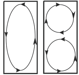
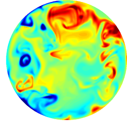
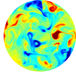
Figure 1: (Color online) a) Sketch of a single roll state (left) and a double roll state (right) of the large scale circulation in a $\Gamma=1/2$ sample. (b,c) Visualization of the temperature field in the horizontal mid-plane of a cylindrical convection cell for Ra=2.91 $\times 10^{8}$ and Pr=4.38 in a $\Gamma=1$ sample ste09 . The red and blue areas indicate warm and cold fluid, respectively. (b) At a slow rotation rate (1/Ro=0.278), and below the transition: The warm up-flow (red) and cold down-flow (blue) reveal the existence of a single convection roll superimposed upon turbulent fluctuations. (c) At a somewhat larger rotation rate (1/Ro=0.775), above the transition: Here, the vertically-aligned vortices cause disorder on a smaller length scale in the horizontal plane.

In order to analyze the sidewall temperature profile Stevens et al. ste10c proposed a quantitative measure for the temperature signature, which they called the relative LSC strength in their study on the effect of plumes on measuring the LSC in samples with $\Gamma=1$ and $\Gamma=1/2$ in non-rotating RB convection. This measure is based on the energy in the different Fourier modes of the measured or computed azimuthal temperature profile at or nearby the sidewall, as

$$\bar{S}_{k}=\mathrm{max}\left(\frac{\frac{N\langle E_{1}\rangle}{\langle E_{tot}\rangle}-1}{N-1},0\right)~{}.$$ (1)

The subscript $k$ indicates the height at which $\bar{S}_{k}$ is determined, that is for $k=b$ at $z/L=0.25$, for $k=m$ at $z/L=0.50$, and for $k=t$ at $z/L=0.75$. In equation (1) $\langle E_{1}\rangle\equiv\int_{t_{b}}^{t_{e}}E_{1}dt$ indicates the sum of the energy in the first Fourier mode over the time interval $[t_{b},t_{e}]$ (from the beginning of the statistically steady part of the simulation at $t=t_{b}$ to the end of the simulation at $t=t_{e}$), and $\langle E_{tot}\rangle$ is defined similarly with $E_{tot}$ being the total energy in all Fourier modes. Furthermore, $N$ is the total number of Fourier modes that can be determined (depending on the number of azimuthal probes). From its definition it follows that $0\leq\bar{S}_{k}\leq 1$. Concerning the limiting values: $\bar{S}_{k}=1$ means the presence of a pure azimuthal cosine profile and $\bar{S}_{k}=0$ indicates that the magnitude of the cosine mode is equal to (or weaker than) the value expected from a random noise signal, see Ref. ste10c . Hence, a value for $\bar{S}_{k}$ of about $0.5$ or higher is a signature that a cosine fit on average is a reasonable approximation of the data set, as then most energy in the signal resides in the first Fourier mode. In contrast, $\bar{S}_{k}$ well below $0.5$ indicates that most energy resides in the higher Fourier modes. In section I.2 we discuss how this method is used to determine the existence of different turbulent states in rotating RB convection.

I.2 Rotating Rayleigh-Bénard convection

The case where the RB system is rotated around its vertical axis at an angular speed $\Omega$ is used to study the effect of rotation on heat transport and flow structuring. Here we define the Rossby number as $Ro=U/(2\Omega L)$, with $U=\sqrt{\beta g\Delta L}$ being the free-fall velocity (mean bulk velocity) to make sure that Ro is the relevant parameter that determines when the formation of large scale vortices sets in. In the remainder of the paper we will indicate the dimensionless rotation rate by 1/Ro as this parameter increases with increasing rotation rate.

Since the experiments by Rossby ros69 it is known that rotation can enhance heat transport. Rossby measured an increase in the heat transport with respect to the non-rotating case of about $10\%$ when water is used as the convective fluid. This increase is counterintuitive as the stability analysis of Chandrasekhar cha81 has shown that rotation delays the onset to convection and from this analysis one would expect that the heat transport decreases. The mechanism responsible for this heat transport enhancement is Ekman pumping ros69 ; jul96b ; vor02 ; kun08b ; kin09 ; zho09b , that is, due to rotation, rising or falling plumes of hot or cold fluid are stretched into vertically-aligned vortices that suck fluid out of the thermal boundary layers adjacent to the bottom and top horizontal plates. Evidence for the existence of vertically-aligned vortices was reported 15-20 years ago bou90 ; zho93 ; sak97 . Sakai was the first who confirmed with flow visualization experiments that there is a typical ordering of vertically-aligned vortices under the influence of rotation. For higher rotation rates a strong heat transport reduction, due to the suppression of the vertical velocity fluctuations by rotation, is found. After Rossby ros69 many experiments have confirmed this general picture qualitatively and, in recent years, also quantitatively, see for example Refs. zho93 ; jul96 ; liu97 ; vor02 ; kun08b ; kin09 ; liu09 ; zho09b ; ste09 ; zho10c ; wei10 ; wei11 ; wei11b ; kun11 .
Next to experiments there have been a number of numerical studies of rotating RB convection kun08b ; kun10 ; kun10b ; kun11 ; zho09b ; wei10 ; ste09 ; ste10a ; ste10b ; ste11b . These studies focussed on the influence of rotation on heat transport and the corresponding changes in the flow structure. Zhong et al. zho09b and Stevens et al. ste09 ; ste10a used results from experiments and simulations in a $\Gamma=1$ sample to study the influence of Ra and Pr on the effect of Ekman pumping, and thus on heat transport.
For an overview of the parameter regimes that are covered in simulations and experiments during the recent decades we refer to the figures 1 of Stevens et al. ste10b ; ste11b . These phase diagrams reveal that there are two approaches to analyze rotating RB convection. The first approach is to vary the rotation rate while the temperature difference between the two horizontal plates is fixed. This means that one varies 1/Ro, while Ra is kept constant. The second approach is to keep the ratio between the viscous force to the Coriolis force, indicated by the Ekman (Ek) or Taylor (Ta) number, fixed. In almost all simulations and experiments the Pr number is kept constant and a fixed Ek number then means that Ra and 1/Ro are varied. This approach is followed by several authors liu97 ; liu09 ; liu11 ; kin09 ; kin12 ; sch09 ; sch10 . Here we take the first approach, that is, vary the rotation rate while the temperature difference between the plates is fixed.

When heat transport enhancement as function of the rotation rate is considered, a typical division in three regimes is observed. Namely regime I (weak rotation), where no heat transport enhancement is observed, regime II (moderate rotation), where a strong heat transport enhancement is found, and regime III (strong rotation), where the heat transport starts to decrease bou90 ; kun10 ; kun11 . Based on an experimental and numerical study on the properties of the LSC in rotating RB in a $\Gamma=1$ sample Kunnen et al. kun08b showed that there is no LSC in regimes II and III. Subsequently, Stevens et al. ste09 showed for a similar setting that the heat transport enhancement at the start of regime II sets in as a sharp transition (at a critical value of the inverse Rossby number, 1/Ro_c). They showed that in experiments the transition is indicated by changes in the time-averaged LSC amplitudes, i.e. the average amplitude of the cosine fit to the azimuthal temperature profile at the sidewall, and the vertical temperature gradient at the sidewall. We note that the formation of a mean vertical temperature gradient in rotating RB convection was already observed earlier, see Refs. jul96 ; har99 . Later experiments and simulations kun11 ; wei11b in a $\Gamma=1$ sample revealed that $\bar{S}_{k}$ is close to one before the onset of heat transport enhancement. In this regime the LSC is the dominant flow structure. After the onset vertically-aligned vortices become the dominant flow structure and then $\bar{S}_{k}$ quickly decreases to zero. The reason is the formation of many randomly positioned vertically-aligned vortices, and due to their random locations, see figure 1c, the cosine mode in the azimuthal temperature profile disappears.

In addition, simulation results have shown that the transition between the two different states is visible not only in the Nu number and the LSC statistics, but also by a strong increase in the number of vortices at the thermal boundary layer height ste09 ; ste11b ; wei10 ; kun10b . In addition, rotation changes the character of the kinetic boundary layer from a Prandtl-Blasius boundary layer at no or weak rotation to an Ekman boundary layer after the onset, which is revealed by the ${1/Ro}^{-1/2}$ scaling of the kinetic boundary layer thickness after the onset for $\Gamma=1$. Furthermore, Stevens et al. ste09 observed for this case an increase in the vertical velocity fluctuations at the edge of the thermal boundary layer, due to the effect of Ekman pumping, while a decrease in the volume averaged vertical velocity fluctuations is found due to the destruction of the LSC.

I.3 Issues addressed in the present paper

Most findings described above are based on experiments and simulations in $\Gamma=1$ samples. In the present paper we study rotating RB convection in an aspect ratio $\Gamma=1/2$ sample as experiments have revealed important differences with respect to the $\Gamma=1$ case. Recently, Weiss and Ahlers wei10b revealed that in such a $\Gamma=1/2$ sample with water (Pr=4.38) at a range of Rayleigh numbers ($2.3\times 10^{9}\leq Ra\leq 7.2\times 10^{10}$) the flow can be either in a single roll (see left panel of figure 1a) or in a double roll state (see right panel of figure 1a) when no rotation is applied. Here, modest rotation (1/Ro$\lesssim$ 1/Ro_c), stabilizes the single roll state and suppresses the double roll state. Surprisingly, computation of $\bar{S}_{k}$ reveals that after the onset of heat transport enhancement at 1/Ro_c the cosine-signature of the temperature profile at the sidewall does not disappear. This may suggest that in a $\Gamma=1/2$ sample the single roll state continues to exist in the rotating regime, whereas it has been shown to disappear in a $\Gamma=1$ sample kun08b ; kun11 ; ste09 ; wei11b . As discussed by Weiss and Ahlers wei11 ; wei11b the value of $\bar{S}_{k}\gtrsim 0.5$ does not allow us to distinguish between a single roll state and a two-vortex state, in which one vortex extends vertically from the bottom into the sample interior and brings up warm fluid, while another vortex transports cold fluid downwards at the opposite part of the cylindrical sample. Such a two-vortex state presumably results in a periodic azimuthal temperature variation close to the sidewall which cannot be distinguished from the temperature signature of a convection roll with up-flow and down-flow near the side wall. It is worthwhile to emphasize the distinction with the $\Gamma=1$ case with 1/Ro$>$1/Ro_c. Here, the vertically-aligned vortices emerging at the bottom plate (transporting hot fluid upwards) are distributed more or less randomly over the horizontal cross section and similarly for the vortex tubes emanating from the top plate.

Table 1: Details for the simulations performed at Ra=$4.52\times 10^{9}$ and Pr=4.38 in an aspect ratio $\Gamma=1/2$ sample. The columns from left to right indicate the Rossby number 1/Ro, the Nusselt number ($Nu_{f}$) obtained after averaging the results of the three methods (see text) using the whole simulation length, and the Nusselt number ($Nu_{h}$) after averaging the results of the three methods over the last half of the simulation. The following column indicates the normalized temperature gradient at the sidewall $\Delta_{w}/\Delta$. The next three columns give the Nusselt number derived from the volume averaged value of the pseudo kinetic dissipation rate $\langle\epsilon_{u}^{"}\rangle$, and the kinetic $\langle\epsilon_{u}\rangle$ and thermal $\langle\epsilon_{\theta}\rangle$ dissipation rates compared to $Nu_{f}$ indicated in column two. The last column indicates the simulation length in dimensionless time units that is considered for the data collection; before this period each simulation has been run for $80-100$ time units in order to prevent transient effects.

1/Ro	$Nu_{f}$	$Nu_{h}$	$\Delta_{w}/\Delta$	$\frac{\frac{\langle\epsilon_{u}^{"}\rangle}{\nu^{3}Ra/(Pr^{2}L^{4})}+1}{Nu_{f}}$	$\frac{\frac{\langle\epsilon_{u}\rangle}{\nu^{3}Ra/(Pr^{2}L^{4})}+1}{Nu_{f}}$	$\frac{\frac{\langle\epsilon_{\theta}\rangle}{\kappa\Delta^{2}/L^{2}}}{Nu_{f}}$	$\tau_{f}$
$0$	103.82	104.03	-0.0848	0.996	0.995	0.976	330
$0.2778$	104.27	103.80	-0.0739	0.985	0.976	0.974	330
$0.3571$	104.89	104.86	-0.0642	0.993	1.019	0.975	330
$0.4651$	105.58	105.45	-0.0645	0.985	0.976	0.973	330
$0.5263$	105.61	105.75	-0.0538	0.988	1.001	0.974	330
$0.5988$	105.86	106.09	-0.0474	1.001	1.000	0.976	330
$0.6897$	105.56	105.41	-0.0529	0.992	0.995	0.975	330
$0.7752$	106.14	105.58	-0.0469	1.002	0.984	0.976	330
$0.8696$	106.66	107.18	-0.0420	1.001	1.014	0.976	306
$1.0000$	106.22	106.03	-0.0547	0.983	0.971	0.974	252
$1.2500$	107.54	107.55	-0.0620	0.999	0.980	0.974	268
$1.5385$	108.49	108.22	-0.0811	0.980	0.990	0.973	282
$2.2222$	111.25	110.91	-0.0862	0.986	0.984	0.973	276
$3.3333$	111.93	112.19	-0.0946	1.002	0.989	0.974	311
$5.0000$	112.23	111.98	-0.1148	0.991	0.986	0.971	330
$8.3333$	111.09	111.38	-0.1272	0.986	0.970	0.969	330
$10.000$	104.97	105.19	-0.1873	1.004	1.047	0.969	487
$12.500$	101.41	102.88	-0.1778	1.006	0.982	0.971	330

From a retrospective point of view we can now conclude that Stevens et al. ste11b already observed some first hints for the presence of a two-vortex state (see figure 5 for an impression of a two-vortex state) in a $\Gamma=1/2$ sample at Ra = $2.91\times 10^{8}$, 1/Ro = 3.33 and Pr = 4.38 (see figure 5a of that paper). However, an open question is whether this state prevails for a considerable time and for different values of Ra, Pr, and a range of rotation rates (in particular matching the settings of the experiments by Weiss and Ahlers wei11 ; wei11b ). Additionally, can we complement the indirect evidence for a two-vortex state as put forward by Weiss and Ahlers wei11 ; wei11b with direct observations of the flow structures in the bulk flow? Can we also distinguish between a genuine two-vortex state and a flow structuring consisting of a few vertically-aligned vortices with hot rising fluid on one side of the cylindrical sample and a few of such vortices bringing cold fluid from the top plate downwards close to the opposite sidewall? In the present paper we report on direct numerical simulation results for $\Gamma=1/2$, Ra = $4.52\times 10^{9}$, and Pr = 4.38 over the range 0 $\lesssim$ 1/Ro $\lesssim$ 12, corresponding to a subset of the Weiss-Ahlers experiments thus allowing direct comparison. The results show that a complex vortex state, which in the time average has the signature of a two-vortex state, persists over the range 1/Ro_c $\lesssim$ 1/Ro $\lesssim$ 12. This confirms that the observation of a sinusoidal azimuthal temperature profile near the sidewall can indeed be explained by the presence of Ekman vortices. In addition, to this general result, we report detailed data that permit a direct comparison of $S_{t}$, $S_{m}$, and $S_{b}$ (see figure 3) and the LSC amplitude (see figure 4) with experiment over a wide 1/Ro range. Furthermore, we also computed the Nusselt number and the vertical temperature gradient at the sidewall (see figure 2). All of these properties show excellent agreement between our simulations and the available experimental measurements; our simulations can therefore be used for exploration of the bulk and boundary layer flow structure which are not accessible in the current experiments.

We first discuss the numerical method in Section II, before we compare the simulation data with the experiments in Section III. In Section IV we discuss flow diagnostics that can only be obtained in simulations and show that in a $\Gamma=1/2$ sample the vertically-aligned vortices arrange such that a sinusoidal azimuthal temperature profile close to the sidewall is formed.

II Numerical method

We simulate rotating RB convection for Ra=$4.52\times 10^{9}$ and Pr=4.38 in an aspect ratio $\Gamma=1/2$ sample by solving the three-dimensional Navier-Stokes equations within the Boussinesq approximation. A constant temperature boundary condition is applied at the horizontal plates, while the sidewall is modeled as adiabatic. This case has been chosen to be as close as possible to the experiments performed by Weiss and Ahlers wei11 ; wei11b . General details about the numerical procedure can be found in Refs. ver96 ; ver99 and specific details concerning the (non)rotating RB simulations in Refs. zho09b ; ste10a .

In order to eliminate the effect of transients we discarded the information of the first $80-100$ dimensionless time units and the simulation lengths we mention refer to the length of the actual simulation, thus the period after this initialization. In Table 1 we compare the Nusselt number averaged over the whole simulation length (denoted by $Nu_{f}$; the Nusselt number is based on the averages of three methods, i.e. the volume average of $Nu=(\langle u_{z}\theta\rangle_{A}-\kappa\partial_{3}\langle\theta\rangle_{A}$)/ $\kappa\Delta L^{-1}$ and the averages based on the temperature gradients at the bottom and top plate) with the Nusselt number averaged over half the simulation length ($Nu_{h}$). For all cases these values $Nu_{f}$ and $Nu_{h}$ are converged within $1\%$.
The simulations have been performed on a grid with $641\times 161\times 641$ nodes in the azimuthal, radial, and axial direction, respectively. The grid allows for a very good resolution of the small scales both inside the bulk of turbulence and in the boundary layers where the grid-point density has been enhanced. We checked this by calculating the Nusselt from the volume-averaged kinetic energy dissipation rate $\langle\epsilon_{u}\rangle=\nu^{3}(Nu-1)Ra/(Pr^{2}L^{4})$, and thermal dissipation rate $\langle\epsilon_{\theta}\rangle=\kappa\Delta^{2}Nu/L^{2}$ as is proposed by Stevens et al. ste10 . In addition, we now also compare with the volume averaged value of $\epsilon_{u}^{"}:=\bf{u}\cdot\nabla^{2}\bf{u}$. The Nusselt number calculated from these quantities is always within a $5\%$ margin, and even much closer for most simulations, of $Nu_{f}$, which according to Stevens et al. ste10 indicates that the simulations are well-resolved, see Table 1 for details. As argued by Shishkina et al. shi10 it is especially important to properly resolve the boundary layers. Our grid-point resolution in the boundary layers also satisfy their criteria for the rotating case (where kinetic boundary layers tend to become thinner with increasing rotation rate).

III Comparison with experiments

In figure 2a we show that the Nusselt number as function of the rotation rate Nu(1/Ro), with respect to the non-rotating value Nu(0), obtained in the simulations agrees excellently with the experimental result of Weiss and Ahlers wei11b . In addition, we note that the absolute values differ less than $1\%$, which can be considered as an excellent agreement. The figure shows that a strong heat transport enhancement due to Ekman pumping sets in at a critical dimensionless rotation rate 1/Ro_c $\approx$ 0.86. For strong rotation rates, i.e. high values of 1/Ro, the expected decrease in the heat transport is observed. In figure 2b, we find that the normalized vertical temperature gradient at the sidewall at $z/L=0.50$, denoted by $\Delta_{w}/\Delta$, and calculated from the azimuthally and time averaged temperatures at the sidewall at $z/L=0.25$ and $z/L=0.75$, is also in good agreement with the measurements by Weiss and Ahlers wei11b .

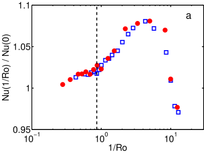
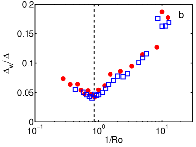
Figure 2: (color online) (a) The heat transfer enhancement with respect to the non-rotating case, Nu(1/Ro)/Nu(0), and (b) the temperature gradient at the sidewall as function of the rotation rate 1/Ro for Ra=$4.52\times 10^{9}$ and Pr=4.38 in a $\Gamma=1/2$ sample. The experimental data from Weiss and Ahlers wei11b are indicated by the blue open squares and the simulation results with the red solid circles. The vertical dashed lines indicates the position of the transition (at 1/Ro_c $\approx$ 0.86) wei10 .

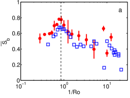
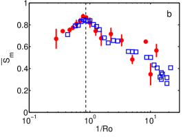
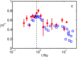
Figure 3: (color online) The values of (a) $\bar{S}_{b}$ (at $0.25z/L$), (b) $\bar{S}_{m}$ (at $0.50z/L$), and (c) $\bar{S}_{t}$ (at $0.75z/L$) as function of 1/Ro. The experimental data from Weiss and Ahlers wei11b are indicated by blue open squares and the simulation results with red solid circles. The experimental and simulation results are for Ra=$4.52\times 10^{9}$ and Pr=4.38 in a $\Gamma=1/2$ sample. For the simulation data $\bar{S}$ is based on the temperature measurements of $64$ azimuthally equally spaced probes outside the sidewall boundary layer and for the experimental data it is based on temperature measurements of $8$ probes embedded in the sidewall. The vertical dashed line indicates the position of 1/Ro_c $\approx$ 0.86 wei10 .

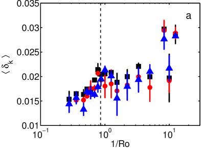
Figure 4: (color online) The time-averaged temperature amplitudes $\langle\delta_{k}\rangle$ for all three levels $k\in\{b,m,t\}$, with the symbols representing $b$ (red circles), $m$ (black squares) and $t$ (blue triangles)} as function of 1/Ro for $\Gamma=1/2$ and Ra=$4.52\times 10^{9}$. Vertical dashed line as in figure 3.

In the simulations we placed $64$ numerical probes at $r=0.95D/2$, which is outside the sidewall boundary layer. The probes are placed some distance from the wall in order to collect data on the velocity components as well, which are all zero at the wall. These velocity data are complementary to the temperature measurements as the region in which a relatively high (low) temperature is measured should correspond to the region with positive (negative) vertical velocity. As we do not want to see the effect of very small plume events we apply a moving averaging filter of $8$ dimensionless time units, see Stevens et al. ste10c for details, to the temperature measurements of the probes, before we determined $\bar{S}_{k}$, with $k\in\{b,m,t\}$. Figure 3a-c shows that the measured $\bar{S}_{k}$ at $z/L=0.25$, $z/L=0.50$, and $z/L=0.75$ in the simulations agree well with the experimental measurements wei11b , which are based on the temperature measurements of just $8$ probes embedded in the sidewall instead of the $64$ numerical probes in our simulations. The error bars in the figure indicate the difference between ${\bar{S}_{k}}$ obtained using the complete time interval with ${\bar{S}_{k}}$ based on the last half of the simulation. Experimental and numerical data obtained in a $\Gamma=1$ sample revealed that ${\bar{S}_{k}}$ strongly decreases to values around ${\bar{S}_{k}}\approx 0.2$ when the heat transport enhancement sets in wei11b . This is obviously not the case in the $\Gamma=1/2$ sample (in general ${\bar{S}_{k}}\approx 0.5$ for 1 $\lesssim$ 1/Ro $\lesssim$ 10, see figure 3). The experimental results do not suggest that this general feature depends on Ra wei11b .

Following Ref. bro06 the orientation and strength of the LSC can be determined by fitting the function $\theta_{i}=\theta_{k}+\delta_{k}\cos(\phi_{i}-\phi_{k})$ to the temperatures recorded by the numerical probes at the height $k\in\{b,m,t\}$, with $b$, $m$, and $t$ defined below Eq. (1). Here, $\phi_{i}=2i\pi/N$, with $N$ the number of probes, refers to the azimuthal position of the probes, and $\delta_{k}$ and $\phi_{k}$ indicate the temperature amplitude and orientation of the LSC, respectively. In figure 4 we plot the time-averaged temperature amplitude $\langle\delta_{k}\rangle$ of the LSC as function of the rotation rate for $\Gamma=1/2$. A comparison with the experimental data of Weiss and Ahlers wei11b (where results are available for both $\Gamma=1/2$ and $\Gamma=1$) shows that within our statistical convergence the trends shown in the numerical data for $\Gamma=1/2$ are similar to those revealed in the experiments (and show a remarkably different trend compared to results for $\Gamma=1$ which show a decreasing $\langle\delta_{k}\rangle$ for increasing rotation wei11b ). The temperature amplitude of the LSC is relatively small for weak rotation (small values of 1/Ro). It becomes slightly larger when increasing the rotation rate from zero to the critical rotation rate (1/Ro_c $\approx$ 0.86). Subsequently, a small dip just after the onset of heat transport enhancement is observed, which is followed by a small further increase in the temperature amplitude.

In summary, in a $\Gamma=1$ sample the transition from the regime with no or weak rotation, with the LSC as the dominant flow structure, to the rotation dominated regime, with vertically-aligned vortices, is indicated by a strong reduction of ${\bar{S}_{k}}$. Also $\langle\delta_{k}\rangle$ decreases with increasing rotation rate also suggesting disappearance of the LSC. In contrast, in a $\Gamma=1/2$ sample these criteria do not provide evidence that the LSC is destroyed at the onset of heat transport enhancement. In the following section we use data that are only available in the simulations to show that also in a $\Gamma=1/2$ sample the LSC is destroyed at the onset of heat transport enhancement and that the vortices arrange such that on average a sinusoidal temperature profile close to the sidewall is still measured.

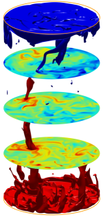
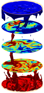
Figure 5: (color online) Flow visualization for Ra=$4.52\times 10^{9}$, Pr=4.38, and 1/Ro=3.33 in an aspect ratio $\Gamma=1/2$ sample. The colormap for the horizontal planes at $z/L=0.25$, $z/L=0.50$, and $z/L=0.75$ is different in panel a and b, and is indicated on the left and right hand side, respectively. The red temperature isosurface, originating from the bottom, indicates the region $\Delta\gtrsim 0.65$, whereas the blue isosurface, originating from the top, indicates the region $\Delta\lesssim 0.35$. Corresponding movies can be found in the supplementary material supplementary .

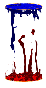
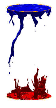
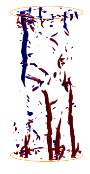
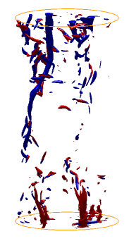
Figure 6: (color online) Flow visualization for Ra=$4.52\times 10^{9}$, Pr=4.38, and 1/Ro=3.33 in an aspect ratio $\Gamma=1/2$ sample The top row shows three-dimensional temperature isosurfaces for two different time instances where the red region indicates $\Delta\gtrsim 0.65$, whereas the blue isosurfaces indicate the region $\Delta\lesssim 0.35$, see figure 5. The bottom row shows a visualization of the vortices, based on the $Q_{3D}$ criterion. Note that the red (blue) regions indicated by the temperature isosurface indeed correspond to vortex regions.

IV Flow structures after transition towards rotation-dominated regime

In this Section we use the availability of all flow data from the simulations to explain why in the rotating regime in an aspect ratio $\Gamma=1/2$ sample the value of ${\bar{S}_{k}}$ does not decrease to values as small as 0.2 or less as usually observed in the $\Gamma=1$ case. In particular, we find that the minimum value is ${\bar{S}_{k}}\approx 0.5$ for 1 $\lesssim$ 1/Ro $\lesssim$ 10 (see figure 3). Only for 1/Ro $\gtrsim$ 10 the experimental data indicate a further substantial decrease of ${\bar{S}_{k}}$ wei11b . Weiss and Ahlers already proposed the idea of a two-vortex state which may explain the temperature profiles measured in their experiments. However, no experimental validation was possible in their experiments. To address this issue we have visualized the flow and temperature field for Ra = $4.52\times 10^{9}$ and Pr=4.38 at 1/Ro = 3.33, see figures 5 (isosurfaces with constant temperature) and 6 (visualization of vortices by means of temperature and vorticity) and the complementary movies. The visualization based on temperature isosurfaces reveals that also at this high Ra number vertically-aligned vortices are formed in the rotation dominated regime. In the corresponding movies one can see that close to the bottom (top) plate several vortices containing warm (cold) fluid are formed. Although several vortices are created close to the horizontal plates only a few vortices are strong enough to reach the horizontal planes (at $z/L=0.25$, $z/L=0.50$ and $z/L=0.75$) so that they can be observed by sidewall temperature probes. Therefore, most of the time we see only a few prevailing vortices at the horizontal plane at midheight. In addition, we notice the non-trivial result that the vortices arrange such that all warm rising vortices tend to cluster on one side of the cell and the sinking cold vortices on the opposite side (contrary to what is observed for $\Gamma=1$). Note that the horizontal planes (at $z/L=0.25$, $z/L=0.50$ and $z/L=0.75$) reveal that the main rising and sinking vortices are surrounded by a warm (cold) region. As these warm and cold regions are formed on opposite sides of the cell this explains the cosine temperature profile that is observed close to the sidewall.
To further confirm that indeed vertically-aligned vortices are formed we analyzed the flow structure in more detail by determining the positions of the vortices by applying a vortex detection algorithm. The fully three-dimensional detection technique is based on the velocity gradient tensor ${\bf\nabla u}=\partial_{i}u_{j}(i,j\in{1,2,3})$. This tensor can be split into a symmetric and antisymmetric part ${\bf\nabla u}=\frac{1}{2}[{\bf\nabla u}+({\bf\nabla u})^{T}]+\frac{1}{2}[{\bf\nabla u}-({\bf\nabla u})^{T}]=S+\Omega$. The $Q_{3D}$ criterion, according to Hunt et al. hun88 , defines a region as vortex when $Q_{3D}\equiv\frac{1}{2}(\|\Omega\|^{2}-\|S\|^{2})>0$, where $\|A\|=\sqrt{Tr(AA^{T})}$ represents the Euclidean norm of the tensor $A$. In practice the threshold value of zero to distinguish between vorticity and strain dominated regions in the flow, and thus identifying vortices, is found to be unsuitable kun10b . Here, we apply a relatively high positive threshold value, identical for all presented snapshots, that is ’matched’ to the temperature isosurfaces that are presented in figure 6 (top row). The position and size of the detected vortex tubes also agree very well with the coherent structures indicated by the temperature isosurfaces, see figure 6. This confirms that the warm and cold regions shown by temperature isosurfaces are indeed vortices. The main difference between the vortices identified with the vortex detection algorithms and the areas indicated by the temperature isosurfaces are the smaller vortices in the middle. These small vortices do not show up when the temperature criterion is used, since their base is not close to the bottom (top) plate where warm (cold) fluid enters the vortices at their base.
We computed the boundary-layer thickness as function of rotation rate and determined averaged root-mean-square velocity fluctuations, as has been done previously for the $\Gamma=1$ case ste09 ; ste10b . Our aim is to confirm directly from flow field data that the flow structure in a $\Gamma=1/2$ sample indeed changes from a regime dominated by the LSC (1/Ro $\lesssim$ 1/Ro_c) to one dominated by vertically-aligned vortices (1/Ro $\gtrsim$ 1/Ro_c).
First of all we determined the kinetic boundary-layer thickness. Like in Ref. ste10b for the $\Gamma=1$ sample the kinetic boundary-layer thickness is approximately constant before the onset of heat transport enhancement sets in at the critical rotation rate 1/Ro_c. After the onset the kinetic boundary-layer thickness scales as (1/Ro)^-0.50, which is in agreement with the scaling expected from Ekman boundary layer theory. The current data for the $\Gamma=1/2$ (not shown here; graph similar as for $\Gamma=1$ ste09 ) thus reveal that the boundary-layer structure changes from a Prandtl-Blasius type boundary layer when no or weak rotation is applied to an Ekman type boundary layer when 1/Ro$>$1/Ro_c. Subsequently, we determined the volume-averaged vertical velocity fluctuations, and the vertical velocity fluctuations at the edge of the thermal boundary layer. Although not shown here, our computations for $\Gamma=1/2$ indicate that the volume-averaged vertical velocity fluctuations slightly increase for 1/Ro $\lesssim$ 1/Ro_c and strongly decrease for 1/Ro $\gtrsim$ 1/Ro_c, thus indicating that the LSC is destroyed.

The strong decrease in the normalized volume-averaged vertical velocity fluctuations coincides with a further increase of the horizontal average at the edge of the thermal boundary layers. The increase of the fluctuations at the boundary-layer height signifies enhanced Ekman transport. Thus these averages provide additional support that the dominant flow structure changes from a LSC to a regime dominated by vertically-aligned vortices. The average arrangement of these few vortices supports the presence of a sinusoidal azimuthal temperature profile at (or close to) the sidewall for $\Gamma=1/2$. This is also the essential and non-trivial difference with the $\Gamma=1$ sample, where the vertically-aligned vortices are distributed randomly.

V Conclusion

We have shown that for $\Gamma=1/2$ and 1/Ro $\gtrsim$ 0.86 there is no single-roll LSC. Instead, we found a complex state of vortices which, in the time average, yields a sinusoidal azimuthal temperature variation observed in the experiment over a wide range of rotation rates. We have compared data from direct numerical simulations performed at Ra=$4.52\times 10^{9}$ with Pr=4.38 (water) in an aspect ratio $\Gamma=1/2$ sample at different rotation rates with the experimental results of Weiss and Ahlers wei11b . We find very close agreement in global properties, i.e. the measured Nusselt number, and local measurements, i.e. the vertical temperature gradient at the sidewall and the behavior of ${\bar{S}_{k}(1/Ro)}$. In contrast to the $\Gamma=1$ case both ${\bar{S}_{k}}$ and the temperature amplitude of the LSC do not indicate any significant changes at the moment that heat transport enhancement sets in. Weiss and Ahlers wei11b already discussed that ${\bar{S}_{k}}$ cannot distinguish between a single roll state and a two-vortex state, in which one vortex extends vertically from the top into the sample interior and brings down cold fluid, while another emanates from the bottom and introduces warm fluid. Here, we resolved this issue and show with a visualization of temperature isosurfaces and with the use of advanced vortex detection algorithms that at high Ra the formation of a flow structure with basically a few dominant vortices leads to a sinusoidal-like azimuthal temperature profile close to the sidewall. This state gives a high value of $\bar{S}_{k}$ at the three measurement heights due to the warm (cold) fluid that spreads out in the horizontal direction (due to horizontal transport of heat, see Stevens et al. ste10b ). This smoothens the temperature peak in the azimuthal temperature profile at the sidewall. The observation that ${\bar{S}_{k}}\approx 0.5$ for very large rotation rates (up to 1/Ro$\approx$ 10) in a $\Gamma=1/2$ sample indicates that the hot and cold vortices on average must align themselves such that the upgoing (warm) and downgoing (cold) vortices are on opposite sides of the cell, but of course a different organization can be formed at certain time instances. This organization of the vertically-aligned vortices in the $\Gamma=1/2$ sample is a non-trivial difference with the $\Gamma=1$ case. There, the vertically-aligned vortices are distributed randomly. We are not sure what physical mechanism causes this difference between a $\Gamma=1$ and $\Gamma=1/2$ sample. At the moment we are considering stereoscopic particle image velocimetry measurements in Eindhoven in order to directly visualize the two-vortex state in a $\Gamma=1/2$ RB sample and to obtain statistics over a much longer time domain than in the simulations. We note that the visualization was not possible in the earlier experiments of Weiss and Ahlers wei11b as these experiments focused on getting an accurate measurement of the heat transport and hope that these results can answer this question.

In experiments Weiss and Ahlers wei11b showed no significant difference between the $\langle E_{1}\rangle/\langle E_{tot}\rangle$ as function of 1/Ro (see figure 5 of their paper) for different Ra. Based on this observation we do not expect a strong Ra number dependence of the $\bar{S}(1/Ro)$ curve at a given aspect ratio. At the moment there are no measurements or simulations available that studied the Pr number dependence of $\bar{S}(1/Ro)$ and new measurements of numerical simulations would be necessary to determine whether there is a strong Pr number effect.

From previous investigations on rotating RB convection in $\Gamma=1$ cells it was concluded that ${\bar{S}_{k}}$ is a good indicator for the presence of the LSC. From the results reported here we conclude that this quantity cannot provide a unique answer whether the LSC is present or not in turbulent rotating convection in $\Gamma=1/2$ samples. The reason for this is that the vortices in a $\Gamma=1/2$ align in such a way that on average a cosine like temperature profile is formed in the azimuthal direction along the sidewall.

- (1) G. Ahlers, S. Grossmann, and D. Lohse, Heat transfer and large scale dynamics in turbulent Rayleigh-Bénard convection, Rev. Mod. Phys. 81, 503 (2009).
- (2) D. Lohse and K. Q. Xia, Small-Scale Properties of Turbulent Rayleigh-Bénard Convection, Annu. Rev. Fluid Mech. 42, 335 (2010).
- (3) E. Brown, A. Nikolaenko, and G. Ahlers, Reorientation of the large-scale circulation in turbulent Rayleigh-Bénard convection, Phys. Rev. Lett. 95, 084503 (2005).
- (4) H. D. Xi, S. Q. Zhou, Q. Zhou, T. S. Chan, and K. Q. Xia, Origin of temperature oscillations in turbulent thermal convection, Phys. Rev. Lett. 102, 044503 (2009).
- (5) R. J. A. M. Stevens, J.-Q. Zhong, H. J. H. Clercx, G. Ahlers, and D. Lohse, Transitions between turbulent states in rotating Rayleigh-Bénard convection, Phys. Rev. Lett. 103, 024503 (2009).
- (6) R. J. A. M. Stevens, H. J. H. Clercx, and D. Lohse, Effect of plumes on measuring the large-scale circulation in turbulent Rayleigh-Bénard convection, Phys. Fluids 23, 095110 (2011).
- (7) H. T. Rossby, A study of Bénard convection with and without rotation, J. Fluid Mech. 36, 309 (1969).
- (8) S. Chandrasekhar, Hydrodynamic and Hydromagnetic Stability (Dover, New York, 1981).
- (9) K. Julien, S. Legg, J. McWilliams, and J. Werne, Hard turbulence in rotating Rayleigh–Bénard convection, Phys. Rev. E 53, R5557 (1996).
- (10) P. Vorobieff and R. E. Ecke, Turbulent rotating convection: an experimental study, J. Fluid Mech. 458, 191 (2002).
- (11) R. P. J. Kunnen, H. J. H. Clercx, and B. J. Geurts, Breakdown of large-scale circulation in turbulent rotating convection, Europhys. Lett. 84, 24001 (2008).
- (12) E. M. King, S. Stellmach, J. Noir, U. Hansen, and J. M. Aurnou, Boundary layer control of rotating convection systems, Nature 457, 301 (2009).
- (13) J.-Q. Zhong, R. J. A. M. Stevens, H. J. H. Clercx, R. Verzicco, D. Lohse, and G. Ahlers, Prandtl-, Rayleigh-, and Rossby-number dependence of heat transport in turbulent rotating Rayleigh-Bénard convection, Phys. Rev. Lett. 102, 044502 (2009).
- (14) B. M. Boubnov and G. S. Golitsyn, Temperature and velocity field regimes of convective motions in a rotating plane fluid layer, J. Fluid Mech. 219, 215 (1990).
- (15) F. Zhong, R. E. Ecke, and V. Steinberg, Rotating Rayleigh-Bénard convection: asymmetrix modes and vortex states, J. Fluid Mech. 249, 135 (1993).
- (16) S. Sakai, The horizontal scale of rotating convection in the geostrophic regime, J. Fluid Mech. 333, 85 (1997).
- (17) K. Julien, S. Legg, J. McWilliams, and J. Werne, Rapidly rotating Rayleigh-Bénard convection, J. Fluid Mech. 322, 243 (1996).
- (18) Y. Liu and R. E. Ecke, Heat transport scaling in turbulent Rayleigh-Bénard convection: effects of rotation and Prandtl number, Phys. Rev. Lett. 79, 2257 (1997).
- (19) Y. Liu and R. E. Ecke, Heat transport measurements in turbulent rotating Rayleigh-Bénard convection, Phys. Rev. E 80, 036314 (2009).
- (20) J.-Q. Zhong and G. Ahlers, Heat transport and the large-scale circulation in rotating turbulent Rayleigh-Bénard convection, J. Fluid Mech. 665, 300 (2010).
- (21) S. Weiss, R. J. A. M. Stevens, J.-Q. Zhong, H. J. H. Clercx, D. Lohse, and G. Ahlers, Finite-size effects lead to supercritical bifurcations in turbulent rotating Rayleigh-Bénard convection, Phys. Rev. Lett. 105, 224501 (2010).
- (22) S. Weiss and G. Ahlers, Heat transport by turbulent rotating Rayleigh-Bénard convection and its dependence on the aspect ratio, J. Fluid. Mech. 684, 407 (2011).
- (23) S. Weiss and G. Ahlers, The large-scale flow structure in turbulent rotating Rayleigh-Bénard convection, J. Fluid. Mech. 688, 461 (2011).
- (24) R. P. J. Kunnen, R. J. A. M. Stevens, J. Overkamp, C. Sun, G. J. F. van Heijst, and H. J. H. Clercx, The role of Stewartson and Ekman layers in turbulent rotating Rayleigh-Bénard convection, J. Fluid. Mech. 688, 422 (2011).
- (25) R. P. J. Kunnen, B. J. Geurts, and H. J. H. Clercx, Experimental and numerical investigation of turbulent convection in a rotating cylinder, J. Fluid Mech. 642, 445 (2010).
- (26) R. P. J. Kunnen, B. J. Geurts, and H. J. H. Clercx, Vortex statistics in turbulent rotating convection, Phys. Rev. E 82, 036306 (2010).
- (27) R. J. A. M. Stevens, H. J. H. Clercx, and D. Lohse, Optimal Prandtl number for heat transfer in rotating Rayleigh-Bénard convection, New J. Phys. 12, 075005 (2010).
- (28) R. J. A. M. Stevens, H. J. H. Clercx, and D. Lohse, Boundary layers in rotating weakly turbulent Rayleigh-Bénard convection., Phys. Fluids 22, 085103 (2010).
- (29) R. J. A. M. Stevens, J. Overkamp, D. Lohse, and H. J. H. Clercx, Effect of aspect-ratio on vortex distribution and heat transfer in rotating Rayleigh-Bénard, Phys. Rev. E 84, 056313 (2011).
- (30) Y. Liu and R. E. Ecke, Local temperature measurements in turbulent rotating Rayleigh-Bénard convection, Phys. Rev. E 84, 016311 (2011).
- (31) E. M. King, S. Stellmach, and J. M. Aurnou, Heat transfer by rapidly rotating Rayleigh-Bénard convection, J. Fluid Mech. 691, 568 (2012).
- (32) S. Schmitz and A. Tilgner, Heat transport in rotating convection without Ekman layers, Phys. Rev. E 80, 015305 (2009).
- (33) S. Schmitz and A. Tilgner, Transitions in turbulent rotating Rayleigh-Bénard convection, Geophysical and Astrophysical Fluid Dynamics 104, 481 (2010).
- (34) J. E. Hart and D. R. Olsen, On the thermal offset in turbulent rotating convection, Phys. Fluids 11, 2101 (1999).
- (35) S. Weiss and G. Ahlers, Turbulent Rayleigh-Bénard convection in a cylindrical container with aspect ratio =0.50 and Prandtl number Pr = 4.38, J. Fluid. Mech. 676, 5 (2011).
- (36) R. Verzicco and P. Orlandi, A finite-difference scheme for three-dimensional incompressible flow in cylindrical coordinates, J. Comput. Phys. 123, 402 (1996).
- (37) R. Verzicco and R. Camussi, Prandtl number effects in convective turbulence, J. Fluid Mech. 383, 55 (1999).
- (38) R. J. A. M. Stevens, R. Verzicco, and D. Lohse, Radial boundary layer structure and Nusselt number in Rayleigh-Bénard convection, J. Fluid. Mech. 643, 49å (2010).
- (39) O. Shishkina, R. J. A. M. Stevens, S. Grossmann, and D. Lohse, Boundary layer structure in turbulent thermal convection and its consequences for the required numerical resolution, New J. Phys. 12, 075022 (2010).
- (40) E. Brown and G. Ahlers, Rotations and cessations of the large-scale circulation in turbulent Rayleigh-Bénard convection, J. Fluid Mech. 568, 351 (2006).
- (41) J. C. R. Hunt, A. Wray, and P. Moin, Eddies, stream, and convergence zones in turbulent flows, Report CTR-S88, Center for Turbulence Research (unpublished).
- (42) See Supplemental Material at [URL will be inserted by publisher] for movie showing the evolution of the main flow structures over time.