Modified Tucker Decomposition for Tensor Network and Fast Linearized Tensor Renormalization Group Algorithm for Two-Dimensional Quantum Spin Lattice Systems

Abstract

We propose a novel algorithm with a modified Tucker decomposition for tensor network that allows for efficiently and precisely calculating the ground state and thermodynamic properties of two-dimensional (2D) quantum spin lattice systems, and is coined as the fast linearized tensor renormalization group (fLTRG). Its amazing efficiency and precision are examined by studying the spin-$1/2$ anisotropic Heisenberg antiferromagnet on a honeycomb lattice, and the results are found to be fairly in agreement with the quantum Monte Carlo calculations. It is also successfully applied to tackle a quasi-2D spin-$1/2$ frustrated bilayer honeycomb Heisenberg model, where a quantum phase transition from an ordered antiferromagnetic state to a gapless quantum spin liquid phase is found. The thermodynamic behaviors of this frustrated spin system are also explored. The present fLTRG algorithm could be readily extended to other quantum lattice systems.

Efficient and accurate numerical methods are very crucial to tackle the strongly correlated quantum lattice systems. Although some analytical techniques and numerical methods have been proposed in the past decades, a large class of intriguing correlated electron and spin models are still intractable owing to the complexity of quantum many-body systems. Several numerical renormalization group (RG) approaches were thus developed, where the density matrix renormalization group DMRG and its finite temperature variant—the transfer matrix renormalization group TMRG have achieved a great success for one-dimensional (1D) systems. Very recently, generalizing the RG-based algorithms to two-dimensional (2D) quantum lattice systems has been remarkably advancing. A few numerical approaches, for instance, the projected entangle pair state (PEPS) PEPS , the tree tensor network (TN) TTN , the multiscale entanglement renormalization ansatz state MERA , the infinite PEPS projection ; projection2 , the tensor renormalization group TRG1 ; TRG2 ; TRG3 , and so on, were proposed, some of which already gained interesting applications (e.g. Refs. [Li, ; Chen, ]). It is noted that most of these algorithms are effective for the ground state properties, but they are still difficultly applied to study the thermodynamics of 2D quantum lattice models.

By incorporating the infinite time-evolving block decimation technique iTEBD , we developed a linearized TRG (LTRG) algorithm LTRG that renders a convenient way to investigate the thermodynamic properties of low-dimensional quantum spin lattice systems. Although the LTRG method is quite efficient and accurate for 1D quantum systems, its cost is relatively high and the performance near a critical point needs careful improvements for 2D quantum systems. Within the framework of LTRG, when the density operator is represented by a TN through Trotter-Suzuki decomposition Trotter , the truncation is needed to prevent from the divergence of dimension of Hilbert space during the imaginary time evolution, which will unavoidably bring errors that become worse in 2D quantum systems. To solve this issue, we note that the Tucker decomposition (TD) Tucker ; TensorD is a nice way to obtain the best lower dimensional approximation of a single tensor, and has wide applications in areas of data compression, image processing, etc. TensorD The algorithms for the TD like the higher-order singular value decomposition HOSVD ; HOSVD1 and higher-order orthogonal iteration (HOOI) HOOI were suggested.

In this work, by extending the HOOI scheme to a TN instead of a single tensor for an optimal truncation, we propose a novel algorithm that allows us to efficiently and accurately simulate not only the ground state but also thermodynamic properties of 2D quantum spin lattice systems in the thermodynamic limit, which is dubbed as the fast LTRG (fLTRG). We find that the computational cost of fLTRG is insensitive to the coordination number without losing the accuracy, which allows for a higher bond dimension cutoff $D_{c}$ when it is applied to 2D and quasi-2D quantum systems. The cost of the fLTRG algorithm is $\sim O(zD_{c}^{3})$, while the LTRG is $\sim O(D_{c}^{3z-3})$, where $z$ is the coordination number. The reliability, efficiency and accuracy of the fLTRG algorithm are examined by studying a spin-1/2 anisotropic Heisenberg antiferromagnet on the honeycomb lattice, whose energy per site, staggered magnetization and specific heat are efficiently and accurately obtained by the fLTRG, and the results are in good agreement with quantum Monte Carlo (QMC) results. To show its powerful performance and flexible scalability, we applied the fLTRG algorithm to a spin-1/2 frustrated bilayer honeycomb Heisenberg model to which the QMC is not directly accessible, and disclosed a quantum phase transition (QPT) from an ordered antiferromagnetic phase to a gapless quantum spin liquid (QSL) in the ground state. The thermodynamic properties of this frustrated spin system are also calculated. Our results manifest that the fLTRG would be very promising to tackle the intractable correlated quantum many-body systems in two and higher dimensions. In what follows, we shall describe the basic procedure of the fLTRG algorithm with a quantum spin system as an example on a honeycomb lattice.

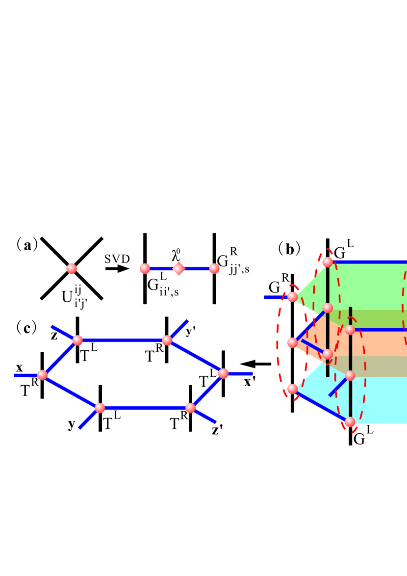
Figure 1: (Color online) (a) The local evolution operator $U^{ij}_{i^{\prime}j^{\prime}}$ is decomposed via an SVD into two gates, $G^{L}_{ij,s}$ and $G^{R}_{i^{\prime}j^{\prime},s}$, each of which has two physical bonds ($i,i^{\prime}$ and $j,j^{\prime}$, black) and one geometrical bond ($s$, blue); (b) Contract the shared physical bonds among $G^{L}$ and $G^{R}$ to get tensors $T^{L}$ and $T^{R}$; (c) A TPDO with inverse temperature $\tau$. Note that the singular value vectors $\lambda^{I,II,III}$ on each geometrical bond is not indicated in (b) and (c) for concise.

Initialization.— Suppose that the Hamiltonian of the system can be written as $H=\sum_{i,j}\hat{H}_{ij}$, where $\hat{H}_{ij}$ is a local Hamiltonian of pairs of spins. The partition function $Z$ is the trace of the density matrix $\rho=\exp(-\beta H)$ with $\beta=1/T$ the inverse temperature and $k_{B}=1$. By means of the Trotter-Suzuki decomposition, the density matrix can be written as $\rho\simeq[\exp{(-\tau\sum_{i,j}\hat{H}_{ij})}]^{K+1}$, where $\beta=(K+1)\tau$, and $\tau$ is the infinitesimal imaginary time slice. Define a local evolution operator $\hat{U}_{ij}=\exp(-\tau\hat{H}_{ij})$. Then, the density operator can be represented as $\rho\simeq[\prod_{i,j}\hat{U}_{ij}]^{K+1}=\prod_{t=1}^{K+1}\prod_{i,j}\hat{U}^{t}_{ij}$, where $t$ is the Trotter index. In this way, the density matrix $\rho$ is transformed into a TN. By making a singular value decomposition (SVD) on $U^{ij}_{i^{\prime}j^{\prime}}=\langle ij|\hat{U}_{ij}|i^{\prime}j^{\prime}\rangle$ where $|ij\rangle$ stands for the direct product basis of spins at site $i$ and $j$, we have $U^{ij}_{i^{\prime}j^{\prime}}=\sum_{s}G^{L}_{ii^{\prime},s}\lambda^{0}_{s}G^{R}_{jj^{\prime},s}$, where $\lambda^{0}$ is the singular value vector, and $G^{L}$ and $G^{R}$ are two local evolution tensors, each of which has two physical bonds ($i,i^{\prime}$ and $j,j^{\prime}$, respectively) and one geometrical bond ($s$). For a honeycomb lattice, this step is depicted in Figs. 1 (a) and (b). Next, by contracting the shared bonds among $G^{L}$ and $G^{R}$ [Fig. 1 (b)], we get

$$T^{L}_{il,xyz}=\sum_{jk}G^{L}_{ij,x}G^{L}_{jk,y}G^{L}_{kl,z},\ T^{R}_{il,xyz}=\sum_{jk}G^{R}_{ij,x}G^{R}_{jk,y}G^{R}_{kl,z},$$ (1)

where $x$, $y$ and $z$ are three inequivalent bonds on a honeycomb lattice [Fig. 1 (c)]. The density operator $\rho$ at an inverse temperature $\tau$ has the form of

$$\rho_{\cdots ii^{\prime}jj^{\prime}\cdots}=Tr_{G}(\cdots\lambda^{II}_{y}\lambda^{III}_{z}T^{L}_{ii^{\prime},xyz}\lambda^{I}_{x}T^{R}_{jj^{\prime},xy^{\prime}z^{\prime}}\lambda^{II}_{y^{\prime}}\lambda^{III}_{z^{\prime}}\cdots),$$ (2)

in which $Tr_{G}$ is the trace over all contracted geometrical bonds, and $\lambda^{I}$, $\lambda^{II}$, $\lambda^{III}$ are three inequivalent singular value vectors with the initial value $\lambda^{0}$. This gives a tensor product density operator (TPDO), which is a direct extension of the matrix product density operator MPDO and the tensor product states. In fact, the TPDO is the infinite product of two inequivalent tensors $T^{L}$ and $T^{R}$ for two sublattices (denoted as $\mathcal{SL}_{a}$ and $\mathcal{SL}_{b}$) of the honeycomb lattice as well as $\lambda^{I}$, $\lambda^{II}$ and $\lambda^{III}$ for three inequivalent bonds [Fig. 1 (c)]. Because of the structure of the present lattice and the forms of interactions, only two inequivalent tensors are adequate here, which is independent of any specific states. For a Kagomé lattice, at least three inequivalent tensors are needed. We now present the fLTRG process on bond $x$ [Fig. 2 (a)] as an example.

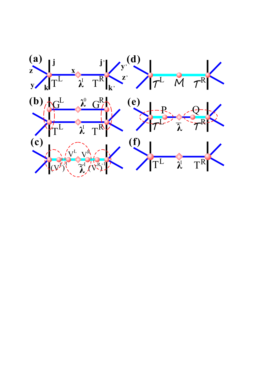
Figure 2: (Color online) (a) A TPDO on bond $x$; (b) acting $G^{L}$ and $G^{R}$ on (a); (c) contracting the non-orthogonal transformation matrices $V^{L}$ and $V^{R}$; (d) obtaining new tensors $\mathcal{T}^{L}$, $\mathcal{T}^{R}$ and matrix ${\cal M}$; (e) decomposing ${\cal M}$ by employing the SVD and contracting the top $D_{c}$ left and right singular vectors $\mathcal{T}^{L}$ and $\mathcal{T}^{R}$, respectively, to obtain the truncated $T^{L}$ and $T^{R}$; and (f) keeping the $D_{c}$ largest singular values as new $\lambda^{I}$.

Evolution.— By acting $G^{L}$ and $G^{R}$ in pairs on the TPDO to evolve along the imaginary time direction, we have

$$\widetilde{T}^{L}_{ik,(xx^{\prime})yz}=\sum_{j}G^{L}_{ij,x^{\prime}}T^{L}_{jk,xyz},\ \widetilde{T}^{R}_{ik,(xx^{\prime})yz}=\sum_{j}G^{R}_{ij,x^{\prime}}T^{R}_{jk,xyz},$$ (3)

as shown in Fig. 2 (b). The dimension of the newly gained bond $(xx^{\prime})$ is enlarged. We denote $(xx^{\prime})$ as an index $\alpha$. Then, the corresponding singular value vector $\widetilde{\lambda}^{I}$ is a direct product of $\lambda^{0}$ and $\lambda^{I}$: $\widetilde{\lambda}^{I}_{\alpha}=\lambda^{0}_{x}\lambda^{I}_{x^{\prime}}$. To obtain the optimal approximation of the TPDO with the truncation of the enlarged bond, we propose a modified HOOI (mHOOI) algorithm. The original HOOI takes the interactions among each mode of a tensor into account by iterating the orthogonal transformation on every bond, implying that the effect of other bonds (or modes) is thus considered when truncating one bond. For our purpose, we suggest the mHOOI algorithm by considering the interactions of not only each bond but also each tensor.

mHOOI.— Define the reduced matrix $M^{L}$ ($M^{R}$) of $\widetilde{T}^{L}$ ($\widetilde{T}^{R}$) on bond $\alpha$ by

$$M^{L}_{\alpha\beta}=\sum_{ikyz}\widetilde{T}^{L}_{ik,\alpha yz}\widetilde{T}^{L}_{ik,\beta yz}\lambda^{II}_{y}\lambda^{III}_{z},\ M^{R}_{\alpha\beta}=\sum_{ikyz}\widetilde{T}^{R}_{ik,\alpha yz}\widetilde{T}^{R}_{ik,\beta yz}\lambda^{II}_{y}\lambda^{III}_{z}.$$ (4)

Making an eigenvalue decomposition on $M^{L}$ and $M^{R}$, we have

$$M^{L}_{\alpha\beta}=\sum_{\chi}\Lambda^{L}_{\alpha\chi}\Gamma^{L}_{\chi}\Lambda^{L}_{\beta\chi},\ M^{R}_{\alpha\beta}=\sum_{\chi}\Lambda^{R}_{\alpha\chi}\Gamma^{R}_{\chi}\Lambda^{R}_{\beta\chi},$$ (5)

where the matrix $\Lambda^{L}$ ($\Lambda^{R}$) is formed by the eigenvectors of $M^{L}$ ($M^{R}$), and $\Gamma^{L}$ ($\Gamma^{R}$) contains the corresponding eigenvalues. The non-orthogonal transformation matrix $V^{L}$ ($V^{R}$) can be obtained by

$$V^{L}_{\alpha\chi}=\Lambda^{L}_{\alpha\chi}\sqrt{\Gamma^{L}_{\chi}},\ \ V^{R}_{\alpha\chi}=\Lambda^{R}_{\alpha\chi}\sqrt{\Gamma^{R}_{\chi}}.$$ (6)

Acting $V^{L}$ and $V^{R}$ to $\widetilde{\lambda}^{I}_{\alpha}$ and their inverses to $\widetilde{T}^{L}$ and $\widetilde{T}^{R}$, respectively, as shown in Figs. 2 (c)-(d), one has

$${\cal M}_{\chi\chi^{\prime}}=\sum_{\alpha}V^{L}_{\alpha\chi}\widetilde{\lambda}^{X}_{\alpha}V^{R}_{\alpha\chi^{\prime}},$$ (7)

$$\mathcal{T}^{L}_{ik,\chi yz}=\sum_{\alpha}\widetilde{T}^{L}_{ik,\alpha yz}(V^{L})^{-1}_{\alpha\chi},$$ (8)

$$\mathcal{T}^{R}_{ik,\chi yz}=\sum_{\alpha}\widetilde{T}^{R}_{ik,\alpha yz}(V^{R})^{-1}_{\alpha\chi}.$$ (9)

It corresponds to inserting two unit matrices [$I=(V^{L})^{-1}\cdot V^{L}=V^{R}\cdot(V^{R})^{-1}$, as shown in Fig. 2 (c)] and changes nothing for the TPDO. The intermediate matrix ${\cal M}$ can be decomposed through SVD as

$${\cal M}_{\chi\chi^{\prime}}=\sum_{\kappa}P_{\chi\kappa}\bar{\lambda}_{\kappa}Q_{\chi^{\prime}\kappa},$$ (10)

where $\bar{\lambda}_{\kappa}$ is the singular value vector arranged in a descending order, $P$ ($Q$) is formed by the left (right) singular vectors of ${\cal M}$. Now, we keep the $D_{c}$ largest singular values as new singular value vector $\lambda^{I}$ of bond $x$, and normalize $\lambda^{I}$ by dividing the renormalization factor $r^{I}_{n}=\sqrt{\sum^{D_{c}}_{i=1}(\lambda^{I}_{i}})^{2}$ with $n$ the step of evolution. Meanwhile, acting the top $D_{c}$ singular vectors in $P$ and $Q$ on $\mathcal{T}^{L}$ and $\mathcal{T}^{R}$, respectively, we get new tensors with truncated bond $x$ [Figs. 2 (e)-(f)]

$$T^{L}_{ik,\kappa yz}=\sum_{\chi}\mathcal{T}^{L}_{ik,\chi yz}P_{\chi\kappa},\ \ T^{R}_{ik,\kappa yz}=\sum_{\chi}\mathcal{T}^{R}_{ik,\chi yz}Q_{\chi\kappa}.$$ (11)

Then we renew $\lambda^{II}$, $\lambda^{III}$ and $\lambda^{I}$ in turn without truncating their dimensions by making the iteration procedure several times (e.g. five times in our case) according to the operations described in Figs. 2 (c)-(f) until reaching a convergence.

fLTRG step.— The evolution and mHOOI processes give a complete fLTRG step on bond $x$. Doing this step on $x$, $y$ and $z$ bonds in one turn corresponds to that the TPDO is evolved with an imaginary time $\tau$. After doing the $Kth$-turn, the inverse temperature for the TPDO reaches $\beta=(K+1)\tau$. Consequently, the density operator $\rho$ is obtained by Eq. (2).

It should be remarked that in the above mHOOI procedure, we first make the truncation on bond $x$ and then do the iteration over three bonds so that the interactions among bonds and tensors are well taken into account. Certainly, one may also iterate first and then truncate the enlarged bond, which gives almost the same result according to our calculations. However, doing the truncation first is obviously more efficient. Moreover, for the present case with an infinite size, we have only three inequivalent bonds on which the iteration goes. In principle, such an mHOOI may also be applied to the finite-size systems by sweeping over all inequivalent bonds to achieve the optimal approximation.

Free energy.— Partition function Z can be obtained by tracing all physical and geometrical bonds. Tracing all physical bonds of the TPDO, we get a 2D classical TN (CTN). The free energy per site $f=-\lim_{N\rightarrow\infty}\ln Z(\beta)/(N\beta)$ with $N$ the number of lattice sites, is comprised of two parts, the renormalization factors $r_{n}^{\mu}$ and the contributed factor per site $r_{2d}$ obtained through the contraction of the CTN:

$$f(\beta)=\frac{1}{2\beta}(\sum^{K}_{n=1}\sum_{\mu=I,II,III}\ln{r^{\mu}_{n}}+2\ln{r_{2d}}).$$ (12)

The thermodynamical quantities including energy, magnetization, susceptibility and specific heat of the 2D quantum systems can thus be obtained.

What is more, the ground state properties can also be studied with the fLTRG algorithm. When one takes $K\rightarrow\infty$ and $\tau\rightarrow 0$, the renormalization factors of each fTRG step converge to $1$. The ground state energy per site $e_{0}$ has a simple form of

$$e_{0}=\lim_{K\rightarrow\infty}\lim_{\tau\rightarrow 0}\frac{1}{2\tau}\ln\prod_{\mu=I,II,III}{{r}^{\mu}}.$$ (13)

Spin-1/2 Heisenberg antiferromagnet on honeycomb lattice. — To test the efficiency and accuracy of the fLTRG algorithm, we employ the spin-$1/2$ anisotropic Heisenberg antiferromagnet on honeycomb lattice in a staggered magnetic field $h_{s}$, and compare the fLTRG results with the QMC calculations QMC . The local Hamiltonian of nearest-neighbor spins reads

$$\hat{H}_{ij}=\delta(\hat{S}^{x}_{i}\hat{S}^{x}_{j}+\hat{S}^{y}_{i}\hat{S}^{y}_{j})+\hat{S}^{z}_{i}\hat{S}^{z}_{j}+(\hat{S}^{z}_{i}-\hat{S}^{z}_{j})h_{s}/3,$$ (14)

where $\hat{S}_{i}^{x}$, $\hat{S}_{i}^{y}$ and $\hat{S}_{i}^{z}$ are the $x$-, $y$- and $z$-component of spin operator on the $i$th site, respectively, and $\delta$ measures the anisotropy of spin couplings. The energy per site can be calculated by $E=-d(\beta f)/d\beta$, and the staggered magnetization per site is obtained by $m_{s}=\partial{f}/\partial{h_{s}}$. Fig. 3 gives $E$ and $m_{s}$ as functions of the inverse temperature $\beta$ for different $\delta$ with $h_{s}=0$ and different $h_{s}$ with $\delta=0.5$, respectively. It can be seen that our fLTRG results are in nice agreement with those of QMC calculations, showing that the fLTRG algorithm is feasible, efficient and accurate.

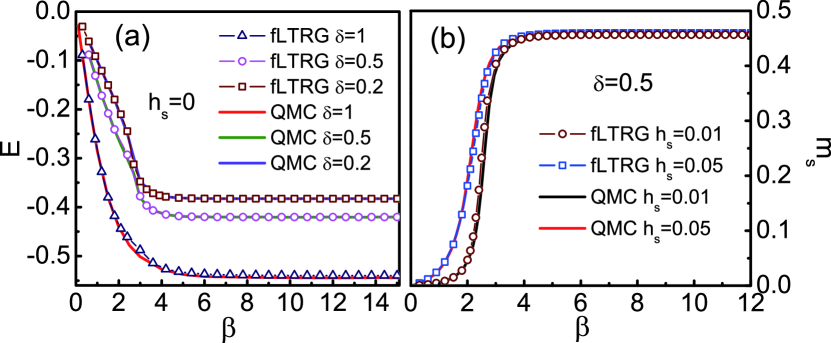
Figure 3: (Color online) The inverse temperature $\beta$ dependence of (a) the energy per site $E$ for different $\delta$ with $h_{s}=0$ and (b) the staggered magnetization per site $m_{s}$ for different $h_{s}$ with $\delta=0.5$ in a spin-$1/2$ anisotropic Heisenberg antiferromagnet on a honeycomb lattice, where $D_{c}=22$ and $\tau=0.005$. The QMC results are also included for comparison.

The specific heat as a function of $\beta$ is calculated by $C=-\beta^{2}dE/d\beta$, as shown in Fig. 4 for $\delta=0.5$. A divergent peak at a critical temperature $T_{c}$ is observed, which indicates that a phase transition occurs between a paramagnetic phase and an antiferromagnetic phase at $T_{c}$. It is also well consistent with the QMC result, showing again the efficiency and accuracy of the fLTRG method. In the inset of Fig. 4, $T_{c}$ as a function of $\delta$ is given, indicating that $T_{c}$ declines almost linearly with increasing $\delta$. It should be pointed out that as $\delta\rightarrow 1$, the divergent peak of the specific heat becomes gradually round owing to the increase of quantum fluctuations, and the phase transition no longer exists at $\delta=1$, being consistent with the Mermin-Wagner theorem.

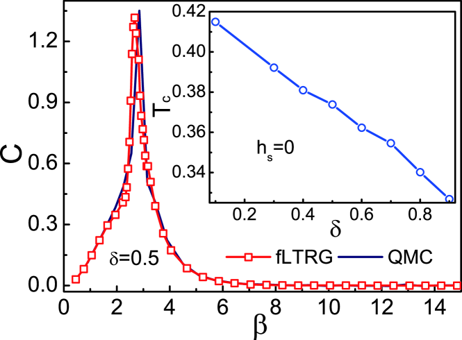
Figure 4: (Color online) The inverse temperature $\beta$ dependence of the specific heat for $\delta=0.5$ and $h_{s}=0$ in a spin-$1/2$ anisotropic Heisenberg antiferromagnet on a honeycomb lattice. The QMC result is included for a comparison. Inset gives the $\delta$ dependence of the critical temperature $T_{c}$. Here $D_{c}=32$.

Spin-1/2 frustrated bilayer honeycomb Heisenberg model. — To show the power of the fLTRG algorithm, we now apply it to investigate the spin-$1/2$ anisotropic Heisenberg antiferromagnetic model on a bilayer honeycomb lattice with alternating antiferromagnetic and ferromagnetic interlayer interactions $J_{a}$ and $J_{b}$ [the inset of Fig. 5 (a)]. It is a quasi-2D quantum frustrated spin system to which the QMC is hardly accessible owing to the negative sign problem. The local Hamiltonian of this model is defined as

$$\hat{H}_{ij}=\hat{H}^{(1)}_{ij}+\hat{H}^{(2)}_{ij}+(\hat{H}^{(a)}_{i}+\hat{H}^{(b)}_{j})/3,$$ (15)

where $\hat{H}^{(\gamma)}_{ij}=J_{\gamma}[\delta_{\gamma}(\hat{S}^{x}_{i}\hat{S}^{x}_{j}+\hat{S}^{y}_{i}\hat{S}^{y}_{j})+\hat{S}^{z}_{i}\hat{S}^{z}_{j}]$, with the layer index $\gamma=1$ and $2$, and $i,j$ the nearest neighbor sites within the single layer; $\hat{H}^{(a,b)}_{i}=J_{a,b}[\delta_{a,b}(\hat{S}^{x}_{i}\hat{S}^{x}_{i}+\hat{S}^{y}_{i}\hat{S}^{y}_{i})+\hat{S}^{z}_{i}\hat{S}^{z}_{i}]$ is the interlayer couplings. When $J_{a}>0$ and $J_{b}<0$, it gives rise to the spin frustration. Without losing generality, we shall take $J_{1}=J_{2}=J>0$, $J_{a}>0$, $J_{b}<0$, $J_{a}=-J_{b}=J^{\prime}$, and $\delta_{1,2}=\delta_{a,b}=\delta=0.5$. As the frustration exists, this model would be expected in proper circumstances to have a QSL ground state that is currently under an active debate Lee ; SL ; SL1 .

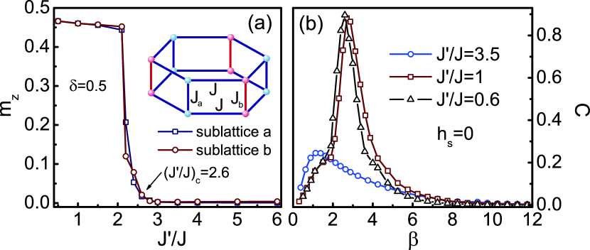
Figure 5: (Color online) (a) The sublattice magnetization per site $m_{z}$ as a function of $J^{\prime}/J$ for a spin-$1/2$ frustrated bilayer honeycomb anisotropic Heisenberg model (inset) with $\delta=0.5$ at zero temperature, where a quantum critical point $(J^{\prime}/J)_{c}=2.60(2)$ is identified. (b) The inverse temperature $\beta$ dependence of the specific heat for different $J^{\prime}/J$ with $h_{s}=0$. Here $D_{c}=32$.

Figure 5 (a) shows the sublattice magnetization per site $m_{z}$ as a function of the coupling ration $J^{\prime}/J$ at zero temperature. It can be seen that there exists a quantum critical point $(J^{\prime}/J)_{c}=2.6$, at which a QPT occurs. When $J^{\prime}/J<2.6$, $m_{z}$ is nonzero and decreases slowly with the increase of $J^{\prime}/J$, showing that in this regime the system is in an antiferromagnetic ordered state; around $J^{\prime}/J\simeq 2.6$, $m_{z}$ drops sharply; and it goes to zero for $J^{\prime}/J>2.6$, while the magnetization in the $x-y$ plane is found about $10^{-3}$ in the whole region, suggesting that the system enters into a disordered state. This disordered state is nothing but a gapless QSL state (see below). The reason is that, for $J^{\prime}/J>2.6$, the frustration becomes stronger note , which strongly suppresses the magnetic long-range ordering, giving rise to a QSL state.

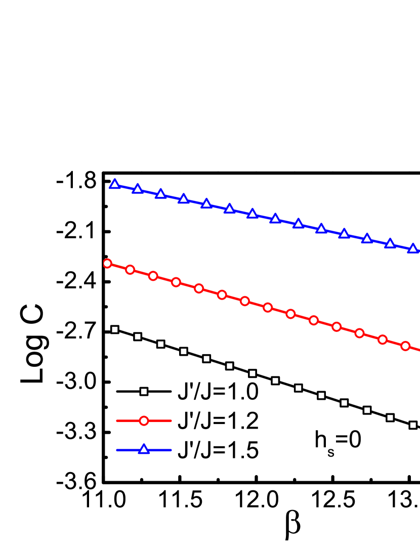
Figure 6: (Color online) (a) Log $C$ versus $\beta$ of the spin-1/2 frustrated bilayer honeycomb Heisenberg model for various $J^{\prime}/J$ with $h_{s}=0$; (b) The gap $\Delta$ versus $J^{\prime}/J$, where the extrapolation shows that at $(J^{\prime}/J)_{c}=2.60(2)$, the gap vanishes, indicating a QPT to a gapless QSL state. Here $D_{c}=35$.

The temperature dependence of the specific heat ($C$) of this frustrated spin system is given for different $J^{\prime}/J$ in Fig. 5 (b). When $J^{\prime}/J<(J^{\prime}/J)_{c}=2.6$, the specific heat displays a divergent peak at a critical temperature for a given $J^{\prime}/J$, showing a second-order phase transition between a paramagnetic state and an Ising-type ordered state. It appears that the critical temperature depends weakly on $J^{\prime}/J$. For $J^{\prime}/J>(J^{\prime}/J)_{c}$, the specific heat shows a round peak, and no phase transition happens, which is consistent with the observation that in this regime the ground state of system is in a gapless QSL state.

Finally, we observe that, when $J^{\prime}/J<2.6$, this frustrated bilayer spin model is in an Ising-type ordered state with a gap. It is evidenced by the low-temperature behavior of the specific heat that decays exponentially with the inverse temperature $\beta$ in a form of $C\thicksim\exp{(-\Delta\beta)}$. The gap $\Delta$ can be determined by using a linear fitting between $\log{C}$ and $\beta$ for different $J^{\prime}/J$ with $h_{s}=0$, as presented in Fig. 6 (a), showing a perfect linear $J^{\prime}/J$ dependence of the gap [Fig. 6 (b)]. By extrapolation, one may observe that $\Delta$ vanishes at $(J^{\prime}/J)_{c}=2.60(2)$, confirming the QPT from a gapped Ising-type ordered state to a gapless QSL state when the frustration effect becomes stronger.

In conclusion, by extending the Tucker decomposition to a tensor network, we propose a novel algorithm coin as the fLTRG, and examine its efficiency and accuracy by employing a spin-$1/2$ Heisenberg antiferromagnet on honeycomb lattice. The fLTRG results are well in agreement with the QMC calculations. To show the power of the fLTRG algorithm, it is applied to a spin-$1/2$ frustrated bilayer honeycomb Heisenberg model with alternating interlayer couplings, and a quantum phase transition is disclosed, where a gapless quantum spin liquid phase is identified. The present fLTRG algorithm could be straightforwardly extended to other quantum lattice systems.

We are indebted to F. Yei, Q. R. Zheng, X. Yan, B. Xi, Y. Zhao and Z. Zhang for stimulating discussions. This work is supported in part by the NSFC (Grant Nos. 90922033 and 10934008), the MOST of China (Grant No. 2012CB932901) and the CAS.

References

- (1) S. R. White, Phys. Rev. Lett. 69, 2863 (1992), Phys. Rev. B. 48, 10345 (1993).
- (2) R. J. Bursill, T. Xiang, and G. A. Gehring, J. Phys. Condens. Matter 8, L583 (1996); X. Q. Wang and T. Xiang, Phys. Rev. B. 56, 5061 (1997).
- (3) F. Verstraete and J. I. Cirac, arXiv:cond-mat/0407066; J. Jordan, R. Orús, G. Vidal, F. Verstraete, and J. I. Cirac, Phys. Rev. Lett. 101, 250602 (2008).
- (4) Y.-Y. Shi, L.-M. Duan, and G. Vidal, Phys. Rev. A 74, 022320 (2006); L. Tagliacozzo, G. Evenbly, and G. Vidal, Phys. Rev. B 80, 235127 (2009).
- (5) G. Vidal, Phys. Rev. Lett. 99, 220405 (2007); Phys. Rev. Lett. 101, 110501 (2008).
- (6) H. C. Jiang, Z. Y. Weng, and T. Xiang, Phys. Rev. Lett. 101, 090603 (2008).
- (7) L. Wang and Frank Verstraete, arXiv:cond-mat/1110.4362v1.
- (8) M. Levin and C. P. Nave, Phys. Rev. Lett. 99, 120601 (2007).
- (9) Z. Y. Xie, H. C. Jiang, Q. N. Chen, Z. Y. Weng, and T. Xiang, Phys. Rev. Lett. 103, 160601 (2009).
- (10) Z. C. Gu, M. Levin, and X. G. Wen, Phys. Rev. B 78, 205116 (2008); Z.C. Gu and X. G. Wen, Phys. Rev. B 80, 155131 (2009).
- (11) P. Chen, C. Y. Lai, and M. F. Yang, J. Stat. Mech. P10001 (2009).
- (12) W. Li, S. S. Gong, Y. Zhao, and G. Su, Phys. Rev. B 81, 184427 (2010); W. Li, S. S. Gong, Y. Zhao, S. J. Ran, S. Gao and G. Su, Phys. Rev. B 82, 134434 (2010).
- (13) G. Vidal, Phys. Rev. Lett. 91, 147902 (2003); Phys. Rev. Lett. 98, 070201 (2007); R. Orús and G. Vidal, Phys. Rev. B 78, 155117 (2008).
- (14) W. Li, S. J. Ran, S. S. Gong, Y. Zhao, B. Xi, F. Ye, and G. Su, Phys. Rev. Lett. 106, 127202 (2011).
- (15) M. Suzuki and M. Inoue, Prog. Theor. Phys. 78, 787 (1987); M. Inoue and M. Suzuki, Prog. Theor. Phys. 79, 645 (1988).
- (16) L. R. Tucker, In Problems in Measuring Change, edited by C. W. Harris (University of Wisconsin Press, Wisconsin, 1963), P122-137.
- (17) T. G. Kolda and B. W. Bader, SIAM Rev. 51, (3) (2009).
- (18) L. R. Tucker, Psychometrika 31, 279-311 (1966).
- (19) L. De Lathauwer, B. De Moor, and J. Vandewalle, SIAM. J. Matrix Anal. and Appl. 21, 1253-1278 (2000).
- (20) L. De Lathauwer, B. De Moor, and J. Vandewalle, SIAM. J. Matrix Anal. and Appl. 21, 1324-1342 (2000).
- (21) F. Verstraete, J. J. Garca-Ripoll, and J. I. Cirac, Phys. Rev. Lett. 93, 207204 (2004).
- (22) A. F. Albuquerque et al., J. Magn. Magn. Mat. 310, 1187 (2007).
- (23) P. A. Lee, Science 321, 1306 (2008).
- (24) S. Yan, D. A. Huse, and S. R. White, Science 332, 1173 (2011).
- (25) G. Evenbly and G. Vidal, Phys. Rev. Lett. 104, 187203 (2010).
- (26) In this bilayer model, the frustration reaches maximum at in the Ising limit.