Robust Lasso with missing and grossly corrupted observations

Abstract

This paper studies the problem of accurately recovering a sparse vector $\beta^{\star}$ from highly corrupted linear measurements $y=X\beta^{\star}+e^{\star}+w$ where $e^{\star}$ is a sparse error vector whose nonzero entries may be unbounded and $w$ is a bounded noise. We propose a so-called extended Lasso optimization which takes into consideration sparse prior information of both $\beta^{\star}$ and $e^{\star}$. Our first result shows that the extended Lasso can faithfully recover both the regression as well as the corruption vector. Our analysis relies on the notion of extended restricted eigenvalue for the design matrix $X$. Our second set of results applies to a general class of Gaussian design matrix $X$ with i.i.d rows $\mathcal{N}(0,\Sigma)$, for which we can establish a surprising result: the extended Lasso can recover exact signed supports of both $\beta^{\star}$ and $e^{\star}$ from only $\Omega(k\log p\log n)$ observations, even when the fraction of corruption is arbitrarily close to one. Our analysis also shows that this amount of observations required to achieve exact signed support is indeed optimal.

I Introduction

One of the central problems in statistics is the problem of linear regression in which the goal is to accurately estimate the regression vector $\beta^{\star}\in\mathbb{R}^{p}$ from the noisy observations

$$y=X\beta^{\star}+w,$$ (1)

where $X\in\mathbb{R}^{n\times p}$ is the measurement or design matrix, and $w\in\mathbb{R}^{n}$ is the stochastic observation vector noise. A particular situation recently attracted much attention from the research community concerns with the model in which the number of regression variables $p$ is larger than the number of observations $n$ ($p\geq n$). In such circumstances, without imposing some additional assumptions for this model, it is obvious that the problem is ill-posed, and thus the linear regression is not consistent. Accordingly, there have been various lines of work on high dimensional inference based on imposing different types of structure constraints such as sparsity and group sparsity (e.g. [1], [2], [3], [4], [5], [6], [7], [8], [9], [10], [11], [12], [13], [14], [15]). Among them, the most popular model focused on sparsity assumption of the regression vector. To estimate $\beta$, a standard method, namely Lasso [1], was proposed to use $l_{1}$-penalty as a surrogate function to enforce sparsity constraint.

$$\min_{\beta}\frac{1}{2n}\left\|y-X\beta\right\|_{2}^{2}+\lambda\left\|\beta\right\|_{1},$$ (2)

where $\lambda$ is the positive regularization parameter and the $\ell_{1}$-norm of the regression vector is $\left\|\beta\right\|_{1}$, defined as $\left\|\beta\right\|_{1}=\sum_{i=1}^{p}|\beta_{i}|$.

Within the past few years, there has been numerous studies to understand the $\ell_{1}$-regularization aspect of sparse regression models (e.g. [5], [6], [7], [8], [9], [10], [11]). These works are mainly characterized by the type of the loss functions considered. For instance, authors [9], [11] seek to obtain a regression estimate $\widehat{\beta}$ that delivers small prediction error while others [10], [6] [11] seek to produce a regressor with minimal parameter estimation error, which is measured by the $\ell_{2}$-norm of $(\widehat{\beta}-\beta^{\star})$. Another line of work (e.g. [16], [5], [8]) considers the variable selection in which the goal is to obtain an estimate that correctly identifies the support of the true regression vector. To achieve low prediction or parameter estimation loss, it is now well known that it is both sufficient and necessary to impose certain lower bounds on the smallest singular values of the design matrix (e.g. [7], [10]), while the notion of small mutual coherence for the design matrix (e.g. [9], [5], [8]) is required to achieve accurate variable selection.

We notice that all previous work relies on the assumption that the observation noise has bounded energy. Without this assumption, it is very likely that the estimated regressor is either not reliable or we fail to identify the correct support. With this observation in mind, in this paper, we extend the linear model (1) by considering the noise with unbounded energy. It is clear that if all entries of $y$ are corrupted by large errors, then it is impossible to faithfully recover the regression vector $\beta^{\star}$. However, in many practical applications such as face recognition, acoustic recognition and dense sensor network, only a portion of the observation vector is contaminated by gross error. Formally, we have the mathematical model

$$y=X\beta^{\star}+e^{\star}+w,$$ (3)

where $e^{\star}\in\mathbb{R}^{n}$ is the sparse error whose locations of nonzero entries are unknown and whose magnitudes can be arbitrarily large whereas $w$ is the conventional noise vector with bounded entries. In this paper, we assume that $w$ has a multivariate Gaussian $\mathcal{N}(0,\sigma^{2}I_{n\times n})$ distribution. This model also includes as a special case the missing data problem in which all the entries of $y$ is not fully observed, but some are missing. This problem is particularly important in computer vision and biology applications. If some entries of $y$ are missing, the nonzero entries of $e^{\star}$ whose locations are associated with the missing entries of the observation vector $y$ have the same values as entries of $y$ but with reverse polarity.

The problems of faithfully recovering data under gross error has gained increasing attentions recently with many interesting practical applications (e.g. [17], [18], [19]) as well as theoretical consideration (e.g. [20], [21], [22], [23]). Another recent line of research on recovering the data from grossly corrupted measurements has been also studied in the context of robust principal component analysis (RPCA) (e.g. [24], [25], [26]). Let us consider several examples as illustrations.

• Face recognition. The model (3) has been proposed by Wright et al. [17] in the context of face recognition. In this problem, a face test sample $y$ is assumed to be represented as a linear combination of training faces in the dictionary $X$. Hence, $y=X\beta$ where $\beta$ is the coefficient vector used for classification. However, it is often the case that the testing face of interest is occluded by unwanted objects such as glasses, hats, scarfs, etc. These occlusions, which occupy a portion of the test face, can be considered as the sparse error $e^{\star}$ in the model (3).

• Subspace clustering. An important problem in high-dimensional data analysis is to cluster the data points into multiple subspaces. A recent work of Elhamifar and Vidal [18] show that this problem can be solved by expressing each data point as a sparse linear combination of all other data points. Coefficient vectors recovered from solving the Lasso problems are then employed for clustering. If the data points are represented as a matrix $X$, then we wish to find a sparse coefficient matrix $B$ such that $X=XB$ and $\operatorname{diag}(B)=0$. When the data is missing or contaminated by outliers, the authors formulate the problem as $X=XB+E$ and minimize a sum of two $\ell_{1}$-norms with respect to both $B$ and $E$ [18].

• Sparse graphical model estimation. Given a random vector $x\in\mathbb{R}^{p}$ with unkown covariance matrix $\Sigma$, the goal is to estimate $\Sigma$ or its precision matrix $\Omega=\Sigma^{-1}$ from $n$ independent copies of $x$: $x_{1},...,x_{n}\in\mathbb{R}^{p}$. Assuming that the matrix $\Omega$ is sparse, Meinshausen and B$\ddot{\text{u}}$hlmann [7] propose to solve the following Lasso problem

  $$\min_{B}\frac{1}{2n}\left\|X-XB\right\|_{F}^{2}+\lambda\left\|B\right\|_{1}\quad\text{s.t. }\operatorname{diag}(B)=0,$$

  where $X=[x_{1}^{T},...,x_{n}^{T}]$. The precision matrix $\Omega$ can be estimated via the coefficient matrix $B$. When the data $X$ is partially observed/missing, a more robust method is to take into account the sparsity assumption and minimize

  $$\min_{B,E}\frac{1}{2n}\left\|X-XB-E\right\|_{F}^{2}+\lambda_{b}\left\|B\right\|_{1}+\lambda_{e}\left\|E\right\|_{1}$$

  subject to $\operatorname{diag}(B)=0$, where $E$ represents partially missing information. Though this problem is quite different from the aforementioned subspace clustering problem, the technical approach is considerably similar.

• Sensor network. In this model, a network of sensors collect measurements of a signal $\beta^{\star}$ independently by simply projecting $\beta^{\star}$ onto the row vectors of a sensing matrix $X$, $y_{i}=\left<X_{i},\beta^{\star}\right>$ [27]. The measurements $y_{i}$ are then sent to the central hub for analysis. However, it is highly likely that a small percentage of sensors might fail to send the measurements correctly and sometimes even report totally irrelevant measurements. Therefore, it is more appropriate to employ the observation model in (3) than the model in (1).

It is worth noticing that in the aforementioned applications, $e^{\star}$ always plays the role as the sparse (undesired) error. However, in other applications, $e^{\star}$ might actually contain meaningful information, and thus necessary to be recovered. An example of this kind of problem is signal separation, in which $\beta^{\star}$ and $e^{\star}$ are considered as two distinct signal components (e.g. video or audio). Furthermore, in applications such as classification and clustering, the assumption that the test sample $y$ is a linear combination of a few training samples in the dictionary (playing the role of the design matrix) $X$ might be violated. The sparse component $e^{\star}$ can thus be seen as the compensation for the linear regression model mismatch.

Given the observation model (1) and the sparsity assumptions on both regression vector $\beta^{\star}$ and error $e^{\star}$, we propose the following convex minimization to estimate the unknown regression vector $\beta^{\star}$ as well as the error vector $e^{\star}$.

$$\min_{\beta,e}\frac{1}{2n}\left\|y-X\beta-e\right\|_{2}^{2}+\lambda_{n,\beta}\left\|\beta\right\|_{1}+\lambda_{n,e}\left\|e\right\|_{1},$$ (4)

where $\lambda_{n,\beta}$ and $\lambda_{n,e}$ are positive regularization parameters. This optimization, which we call extended Lasso, can be seen as a generalization of the Lasso program. Indeed, by setting $\lambda_{n,e}=0$, (6) returns to the standard Lasso. The additional regularization associated with the error $e$ encourages sparsity of the reconstructed vector, where the penalty parameter $\lambda_{n,e}$ controls its sparsity level. In this paper, we focus on the following questions: what are necessary and sufficient conditions for the ambient dimension $p$, the number of observations $n$, the sparsity index $k$ of the regression $\beta^{\star}$ and the fraction of corruption in $e^{\star}$ so that (i) the extended Lasso is able (or unable) to recover the exact support sets of both $\beta^{\star}$ and $e^{\star}$? (ii) the extended Lasso is able to recover $\beta^{\star}$ and $e^{\star}$ with small prediction error and parameter error? We are particularly interested in understanding the asymptotic situation where the the fraction of error gets arbitrarily close to $100\%$.

In this paper, we assume normalization of the design matrix $X$. Specifically, we assume the $\ell_{2}$-norm of columns of the matrix $X$ are $\Theta(\sqrt{n})$. Moreover, without loss of generality, we use the following observation model in replacement for the model in (3)

$$y=X\beta^{\star}+\sqrt{n}e^{\star}+w.$$ (5)

As we can see, columns of both the design matrix $X$ and the matrix $\sqrt{n}I_{n\times n}$ has the same scale. Thus, this model’s change only helps our results in the next sections to be more interpretable. The optimization (4) is now converted to the following problem

$$\min_{\beta,e}\frac{1}{2n}\left\|y-X\beta-\sqrt{n}e\right\|_{2}^{2}+\lambda_{n,\beta}\left\|\beta\right\|_{1}+\lambda_{n,e}\left\|e\right\|_{1},$$ (6)

Previous work. The problem of recovering the estimation vector $\beta^{\star}$ and error $e^{\star}$ is originally proposed by Wright et al. in the appealing paper [17] and analyzed by Wright and Ma [20]. In the absence of the stochastic noise $w$ in the observation model (3), the authors propose to estimate ($\beta^{\star},e^{\star}$) by solving the following linear program

$$\min_{\beta,e}\left\|\beta\right\|_{1}+\left\|e\right\|_{1}\quad\text{s.t.}\quad y=X\beta+\sqrt{n}e.$$ (7)

From a different viewpoint, in the intriguing paper [28], Lee et al. study a general loss function model. To obtain more flexibility in controlling the undesirable influence of the model, they introduce a case-specific parameter vector $e\in\mathbb{R}^{n}$ for the observation vectors and modify the optimization to take into account this parameter. Interestingly, the model turns out to be coincident with (6) when applying to the linear regression problem with Lasso penalty. Extensive simulations have shown that the model (6) is considerably robust to noise. However, no theoretical analysis is provided in the paper.

In another direction, the problem of robust Lasso under corrupted observations is also carefully investigated by Wang et al. [29]. In this appealing paper, instead of using the quadratic loss function as in Lasso, the authors propose to employ LAD-Lasso criterion:

$$\min_{\beta}\left\|y-X\beta\right\|_{1}+\sum_{j=1}^{p}\lambda_{j}|x_{j}|.$$ (8)

This optimization combines the LAD criterion and Lasso penalty, where the first term is designed to be robust to outliers and the second term again promotes the sparse representation of the estimator. However, due to the lack of the quadratic loss that enforce the estimation to be consistence with the observation in $\ell_{2}$-norm sense, this optimization might not guarantee to deliver a solution that satisfies small prediction error.

On the theoretical side, the result of [20] is asymptotic in nature. The analysis reveals that for a class of Gaussian design matrix with i.i.d entries, the optimization (7) can recover $(\beta^{\star},e^{\star})$ precisely with high probability even when the fraction of corruption is arbitrarily close to one. However, the result only holds under rather stringent conditions. In particularly, the authors require the number of observations $n$ grow proportionally with the ambient dimension $p$, and the sparsity index $k$ is a very small portion of $n$. These conditions is of course far from the optimal bound in compressed sensing (CS) and statistics literature (recall $k\leq O(n/\log p)$ is sufficient in conventional analysis (e.g. [30], [8]).

Another line of work has also focused on the optimization (7). In both Laska et al. [19] and Li et al., [21], the authors establish that for Gaussian design matrix $X$, if $n\geq C(k+s)\log p$ where $s$ is the sparsity level of $e^{\star}$, then the recovery is exact. This follows from the fact that the combination matrix $[X,\text{ }I]$ obeys the restricted isometry property, a well-known property in compressed sensing used to guarantee exact recovery of sparse vectors via $\ell_{1}$-minimization. These results, however, do not allow the fraction of corruption to come close to unity. Also related to our paper is recent work by Studer et al., [31] [32] in which the authors establish different results for deterministic design matrix.

Among the previous work, the most closely related to our current paper are recent results by Li [23] and Nguyen et al. [22] in which a positive regularization parameter $\lambda$ is employed to control the sparsity of $e^{\star}$. Using different methods, both sets of authors show that as $\lambda$ is deterministically selected to be $1/\sqrt{\log p}$ and $X$ is a sub-orthogonal matrix, whose columns are selected uniformly at random from columns of an orthogonal matrix, then the solution of following optimization (9) is exact even a constant fraction of observation is corrupted. Moreover, [23] establishes a similar result with Gaussian design matrix in which the number of observations is only on the order of $k\log p$ $-$ a level that is known to be optimal in both CS and statistics community.

$$\min_{\beta,e}\left\|\beta\right\|_{1}+\lambda\left\|e\right\|_{1}\quad\text{s.t.}\quad y=X\beta+\sqrt{n}e.$$ (9)

Our contribution. This paper considers a general setting in which the observations are contaminated by both sparse and dense errors. We allow the corruptions to linearly grow with the number of observations and have arbitrarily large magnitudes. We establish a general scaling of the quadruplet $(n,p,k,s)$ such that the proposed extended Lasso stably recovers both the regression and the corruption vector. Of particular interest to us are the answer to the following questions:

1. First, under what scalings of $(n,p,k,s)$ does the extended Lasso obtain the unique solution with small estimation error?

2. Second, under what scalings of $(n,p,k)$ does the extended Lasso obtain the exact signed support recovery even when almost all observations are corrupted?

3. Third, under what scalings of $(n,p,k,s)$ that no solution of the extended Lasso specifying the correct signed support exists?

To answer for the first question, we introduce a notion of extended restricted eigenvalue for a matrix $[X,\text{ }I]$ where $I$ is the identity matrix. We show that this property is satisfied for a general class of random Gaussian design matrices. The answers to the last two questions requires stricter conditions on the design matrix. In particular, for random Gaussian design matrix with i.i.d rows $\mathcal{N}(0,\Sigma)$, we rely on two standard assumptions: invertibility and mutual incoherence. Our analysis in this setting is relied on the elegant technique introduced by Wainwright [8].

If we denote $Z=[X,\text{ }I]$ where $I$ is an identity matrix and $\overline{\beta}=[\beta^{\star^{T}},\text{ }e^{\star^{T}}]^{T}$, then the observation vector $y$ is reformulated as $y=Z\overline{\beta}+w$, which is the same as the standard Lasso model. However, previous results (e.g. [10], [8]) applying to random Gaussian design matrix are irrelevant to this setting since $Z$ no longer behaves like a Gaussian matrix. To establish the theoretical analysis, we need a deeper study on the interaction between the Gaussian and identity matrices. By exploiting the fact that the matrix $Z$ consists of two components where one has a special structure, our analysis reveals an interesting phenomenon: extended Lasso can accurately recover both the regressor $\beta^{\star}$ and the corruption $e^{\star}$ even when the fraction of corruption is up to $100\%$. We measure the recoverability of these variables under two criterions: parameter accuracy and feature selection accuracy. Moreover, our analysis can be extended to the situation in which the identity matrix can be replaced by a tight frame $D$ as well as extended to other models such as group Lasso or matrix Lasso with sparse error.

Notation. We summarize here some standard notation employed throughout the paper. We reserve $T$ and $S$ as the sparse support of $\beta^{\star}$ and $e^{\star}$, respectively. Given a design matrix $X\in\mathbb{R}^{n\times p}$ and subsets $S$ and $T$, we use $X_{ST}$ to denote the $|S|\times|T|$ submatrix obtained by extracting those rows indexed by S and columns indexed by $T$. For a vector $h\in\mathbb{R}^{p}$, we use the conventional notations for $\ell_{1}$- and $\ell_{2}$-norm of $h$ as $\left\|h\right\|_{1}=\sum_{i=1}^{p}|h_{i}|$ and $\left\|h\right\|_{2}=(\sum_{i=1}^{p}h_{i}^{2})^{1/2}$, respectively. For a matrix $X\in\mathbb{R}^{n\times p}$, we denote $\left\|X\right\|$ and $\left\|X\right\|_{\infty}$ as the operator norms. In particular, $\left\|X\right\|$ is denoted as the spectral norm and $\left\|X\right\|_{\infty}$ as the $\ell_{\infty}/\ell_{\infty}$ operator norm: $\left\|X\right\|_{\infty}=\max_{i}\sum_{j=1}^{p}|x_{ij}|$.

We use the notation $C_{1},C_{2},c_{1},c_{2},$ etc., to refer to positive constants, whose value may change from line to line. Given two functions $f$ and $g$, the notation $f(n)=\mathcal{O}(g(n))$ means that there exists a constant $c<+\infty$ such that $f(n)\leq cg(n)$; the notation $f(n)=\Omega(g(n))$ means that $f(n)\geq cg(n)$ and the notation $f(n)=\Theta(g(n))$ means that $f(n)=\mathcal{O}(g(n))$ and $f(n)=\Omega(g(n))$. The symbol $f(n)=o(g(n))$ indicates that $f(n)/g(n)\rightarrow 0$.

Organization. The remainder of this paper is structured as follows. Section II provides the main results, detailed discussions and their consequences. Section III performs extensive experiments to validate theoretical results presented in the previous section. Section IV provides analysis of the estimation error, whereas Sections V and VI deliver proofs of the necessary and sufficient conditions for the exact signed support recovery. Several technical aspects of these proofs and some well-known concentration inequalities are presented in the Appendix. We conclude the paper in Section VII with more discussion.

II Main results

In this section, we provide precise statements for the main results of this paper. In the first sub-section, we establish the parameter estimation and provide a deterministic result which is based on the notion of extended restricted eigenvalue. We further show that the random Gaussian design matrix satisfies this property with high probability. The next sub-section considers feature estimation. We establish conditions for the design matrix such that the solution of the extended Lasso has the exact signed supports.

II-A Parameter estimation

As in conventional Lasso, to obtain a low parameter estimation bound, it is necessary to impose conditions on the design matrix $X$. In this paper, we introduce the notion of extended restricted eigenvalue (extended RE) condition. Let $\mathbb{C}$ be a restricted set, we say that the matrix $X$ satisfies the extended RE assumption over the set $\mathbb{C}$ if there exists some $\kappa_{l}>0$ such that

$$\frac{1}{\sqrt{n}}\left\|Xh+\sqrt{n}f\right\|_{2}\geq\kappa_{l}(\left\|h\right\|_{2}+\left\|f\right\|_{2})\quad\text{for all }(h,f)\in\mathbb{C},$$ (10)

where the restricted set $\mathbb{C}$ of interest is defined with $\lambda:=\frac{\lambda_{n,e}}{\lambda_{n,\beta}}$ as follows

$$\mathbb{C}:=\{(h,f)\in\mathbb{R}^{p}\times\mathbb{R}^{n}\text{ }|\\ \text{ }\left\|h_{T^{c}}\right\|_{1}+\lambda\left\|f_{S^{c}}\right\|_{1}\leq 3\left\|h_{T}\right\|_{1}+3\lambda\left\|f_{S}\right\|_{1}\}.$$ (11)

This assumption is a natural extension of the restricted eigenvalue condition and restricted strong convexity considered in [10] ,[33] and [34]. In the absence of a vector $f$ in the equation (10) and in the set $\mathbb{C}$, this condition returns to the restricted eigenvalue defined in [10]. As discussed in more detail in [10] and [35], restricted eigenvalue is among the weakest assumption on the design matrix such that the solution of the Lasso is consistent.

With this assumption at hand, we now state the first theorem

Theorem 1.

Consider the optimal solution $(\widehat{\beta},\widehat{e})$ to the optimization problem (6) with regularization parameters chosen as

$$\lambda_{n,\beta}=\frac{2}{\gamma}\frac{\left\|X^{*}w\right\|_{\infty}}{n}\quad\text{and}\quad\lambda_{n,e}=\frac{2\left\|w\right\|_{\infty}}{\sqrt{n}},$$ (12)

where $\gamma\in(0,1]$. Assuming that the design matrix $X$ obeys the extended RE, then the error set $(h,f)=(\widehat{\beta}-\beta^{\star},\widehat{e}-e^{\star})$ is bounded by

$$\left\|h\right\|_{2}+\left\|f\right\|_{2}\leq 3\kappa^{-2}_{l}\left(\lambda_{n,\beta}\sqrt{k}+\lambda_{n,e}\sqrt{s}\right).$$ (13)

There are several interesting observations from this theorem

1) The error bound naturally split into two components related to the sparsity indices of $\beta^{\star}$ and $e^{\star}$. In addition, the error bound contains three quantity: the sparsity indices, regularization parameters, and the extended RE constant. If the terms related to the corruption $e^{\star}$ are omitted, then we obtain similar parameter estimation bound as in the standard Lasso (e.g. [10], [34]).

2) The choice of regularization parameters $\lambda_{n,\beta}$ and $\lambda_{n,e}$ can be made explicitly: assuming $w$ is a Gaussian random vector whose entries are $\mathcal{N}(0,\sigma^{2})$ and the design matrix has $\sqrt{n}$-normed columns, it is clear that with high probability, $\frac{1}{n}\left\|X^{*}w\right\|_{\infty}\leq 2\sqrt{\frac{\sigma^{2}\log p}{n}}$ and $\frac{1}{\sqrt{n}}\left\|w\right\|_{\infty}\leq 2\sqrt{\frac{\sigma^{2}\log n}{n}}$. Thus, it is sufficient to select $\lambda_{n,\beta}\geq\frac{4}{\gamma}\sqrt{\frac{\sigma^{2}\log p}{n}}$ and $\lambda_{n,e}\geq 4\sqrt{\frac{\sigma^{2}\log n}{n}}$.

3) At the first glance, the parameter $\gamma$ does not seem to have any meaningful interpretation and the setting $\gamma=1$ seems to be the best selection due to the smallest estimation error it can produce. However, this parameter actually controls the sparsity level of the regression vector with respect to the fraction of corruption. This relation is enforced via the restricted set $\mathbb{C}$.

In the following lemma, we show that the extended RE condition actually exists for a large class of random Gaussian design matrix whose rows are i.i.d zero mean with covariance $\Sigma$. Before stating the lemma, let us define some quantities operating on the covariance matrix $\Sigma$: $C_{\min}:=\lambda_{\min}(\Sigma)$ is the smallest eigenvalue of $\Sigma$; $C_{\max}:=\lambda_{\max}(\Sigma)$ is the largest eigenvalue of $\Sigma$; and $\xi(\Sigma):=\max_{i}\Sigma_{ii}$ is the maximal entry on the diagonal of the matrix $\Sigma$.

Lemma 1.

Consider the random Gaussian design matrix whose rows are i.i.d $\mathcal{N}(0,\Sigma)$ and assume $C_{\max}\xi(\Sigma)=\Theta(1)$. Select

$$\lambda:=\frac{\gamma}{\sqrt{\xi(\Sigma)}}\sqrt{\frac{\log n}{\log p}}.$$ (14)

Then with probability greater than $1-c_{1}\exp(-c_{2}n)$, the matrix $X$ satisfies the extended RE with parameter $\kappa_{l}=\frac{1}{4\sqrt{2}}$, provided that $n\geq C\frac{\xi(\Sigma)}{C_{\min}}k\log p$ and $s\leq\min\left\{C_{1}\frac{n}{\gamma^{2}\log n},C_{2}n\right\}$ for some small constants $C_{1}$, $C_{2}$.

We would like to offer a few remarks:

1) The choice of parameter $\lambda$ is nothing special here. When the design matrix is Gaussian and independent with the Gaussian stochastic noise $w$, we can easily show that $\frac{1}{n}\left\|X^{*}w\right\|_{\infty}\leq 2\sqrt{\xi(\Sigma)\delta^{2}\log p}$ with probability at least $1-2\exp(-\log p)$. Therefore, the selection of $\lambda$ follows from Theorem 1.

2) The proof of this lemma, shown in the Appendix, boils down to controling two terms

• Restricted eigenvalue with $X$.

  $$\frac{1}{n}\left\|Xh\right\|^{2}_{2}+\left\|f\right\|_{2}^{2}\geq\kappa_{r}(\left\|h\right\|^{2}_{2}+\left\|f\right\|^{2}_{2})\quad\text{for all }(h,f)\in\mathbb{C}.$$

• Mutual incoherence. The column space of the matrix $X$ is incoherent with the column space of the identity matrix. That is, there exists some $\kappa_{m}>0$ such that

  $$\frac{1}{\sqrt{n}}|\left<Xh,f\right>|\leq\kappa_{m}(\left\|h\right\|_{2}+\left\|f\right\|_{2})^{2}\quad\text{for all }(h,f)\in\mathbb{C}.$$

If the incoherence between these two column spaces is sufficiently small such that $4\kappa_{m}<\kappa_{r}$, then we can conclude that $\left\|Xh+f\right\|_{2}^{2}\geq(\kappa_{r}-2\kappa_{m})(\left\|h\right\|_{2}+\left\|f\right\|_{2})^{2}$. The small mutual incoherence property is especially important since it provides how the regression separates itself away from the sparse error.

3) To simplify our result, we consider a special case of the uniform Gaussian design, in which $\Sigma=I_{p\times p}$. In this situation, $C_{\min}=C_{\max}=\xi(\Sigma)=1$. We have the following result which is a corollary of Theorem 1 and Lemma 1

Corollary 1 (Standard Gaussian design).

Let $X$ be a standard Gaussian design matrix. Consider the optimal solution $(\widehat{\beta},\widehat{e})$ to the optimization problem (6) with regularization parameters chosen as

$$\lambda_{n,\beta}=\frac{4}{\gamma}\sqrt{\frac{\sigma^{2}\log p}{n}}\quad\text{and}\quad\lambda_{n,e}=4\sqrt{\frac{\sigma^{2}\log n}{n}},$$ (15)

for $\gamma\in(0,1]$. Also, assuming that $n\geq Ck\log p$ and $s\leq\min\{C_{1}\frac{n}{\gamma^{2}\log n},C_{2}n\}$ for some small constants $C,C_{1},C_{2}$, Then with probability greater than $1-c_{1}\exp(-c_{2}n)$, the error set $(h,f)=(\widehat{\beta}-\beta^{\star},\widehat{e}-e^{\star})$ is bounded by

$$\left\|h\right\|_{2}+\left\|f\right\|_{2}\leq 384\left(\frac{1}{\gamma}\sqrt{\frac{\sigma^{2}k\log p}{n}}+\sqrt{\frac{\sigma^{2}s\log n}{n}}\right).$$ (16)

Corollary 1 reveals a remarkable result: by setting $\gamma=1/\sqrt{\log n}$, even when the fraction of corruption is linearly proportional with the number of samples $n$, the extended Lasso (6) is still capable of recovering both coefficient vector $\beta^{\star}$ and corruption (missing) vector $e^{\star}$ within a bounded error (16). Without the dense noise $w$ in the observation model (3) ($\sigma=0$), the extended Lasso actually recovers the exact solution. This is impossible to achieve with the standard Lasso. Furthermore, if we know in prior that the number of corrupted observations is on the order of $\mathcal{O}(n/\log p)$, then selecting $\gamma=1$ instead of $1/\log n$ will minimize the estimation error (see equation (16)) of Theorem 1.

II-B Feature selection with random Gaussian design

In many applications, the feature selection criterion is more preferred [8] [5]. Feature selection refers to the property that the recovered parameter has the same signed support as the true regressor. In general, good feature selection implies good parameter estimation but the reverse direction does not usually hold. In this part, we investigate conditions for the design matrix and the scaling of $(n,p,k,s)$ such that both regression and sparse error vectors satisfy these criterion.

Consider the linear model (3) where $X$ is the Gaussian random design matrix whose rows are i.i.d zero mean with covariance matrix $\Sigma$. It has been well known in the Lasso that in order to obtain feature selection accuracy, the covariance matrix $\Sigma$ must obey two properties: invertibility and small mutual incoherence restricted on the set $T$. The first property guarantees that (6) is strictly convex, leading to the unique solution of the convex program, while the second property requires the separation between two components of $\Sigma$, one related to the set $T$ and the other to the set $T^{c}$ must be sufficiently small.

1. Invertibility. To guarantee uniqueness, we require $\Sigma_{TT}$ to be invertible. Particularly, let $C_{\min}=\lambda_{\min}(\Sigma_{TT})$, we require $C_{\min}>0$.

2. Mutual incoherence. For some $\gamma\in(0,1)$,

   $$\left\|\Sigma^{*}_{T^{c}T}(\Sigma_{TT})^{-1}\right\|_{\infty}\leq(1-\gamma).$$ (17)

   It is worth noting that these two invertibility and mutual incoherence properties are exactly the same as the conditions used to establish the exact signed support recovery in the standard Lasso (e.g [16], [8], [5]).

Toward the end, we will also elaborate on three other quantities operating on the restricted covariance matrix $\Sigma_{TT}$: $C_{\max}$, which is defined as the maximum eigenvalue of $\Sigma_{TT}$: $C_{\max}:=\lambda_{\max}(\Sigma_{TT})$; and $D^{-}_{\max}$ and $D^{+}_{\max}$, which are denoted as $\ell_{\infty}$-norm of matrices $\Sigma_{TT}^{-1}$ and $\Sigma_{TT}$ : $D^{-}_{\max}:=\left\|(\Sigma_{TT})^{-1}\right\|_{\infty}$ and $D^{+}_{\max}:=\left\|\Sigma_{TT}\right\|_{\infty}$.

Our result also involves two other quantities operating on the conditional covariance matrix of $(X_{T^{c}}|X_{T})$ defined as

$$\Sigma_{T^{c}|T}:=\Sigma_{T^{c}T^{c}}-\Sigma_{T^{c}T}\Sigma_{TT}^{-1}\Sigma_{TT^{c}}.$$ (18)

They are defined as $\rho_{u}(\Sigma_{T^{c}|T})=\max_{i}(\Sigma_{T^{c}|T})_{ii}$ and $\rho_{l}(\Sigma_{T^{c}|T})=\frac{1}{2}\min_{i\neq j}[(\Sigma_{T^{c}|T})_{ii}+(\Sigma_{T^{c}|T})_{jj}-2(\Sigma_{T^{c}|T})_{ij}]$, which we often denote with the shorthand notation $\rho_{u}$ and $\rho_{l}$.

We establish the following result for Gaussian random design whose covariance matrix $\Sigma$ obeys the two assumptions.

Theorem 2 (Achievability).

Given the linear model (3) with random Gaussian design and the covariance matrix $\Sigma$ satisfying invertibility and incoherence properties for any $\gamma\in(0,1)$, suppose that we solve the extended Lasso (6) with regularization parameters obeying

$$\lambda_{n,\beta}=\frac{8}{\gamma}\sqrt{\frac{\sigma^{2}\eta\log n\log p}{n}\max\{\rho_{u},D^{+}_{\max}\}}$$ (19)

$$\text{and}\quad\quad\lambda_{n,e}=4\sqrt{\frac{\sigma^{2}\log n}{n}},$$ (20)

for some $\eta\in[\frac{1}{\log n},1)$. Assume that the sequence (n, p, k, s) and regularization parameters $\lambda_{n,\beta}$, $\lambda_{n,e}$ satisfying $s\leq\eta n$ and $n>\max\{n_{1},n_{2}\}$ where $n_{1}$ and $n_{2}$ are defined as

$$n_{1}:=\frac{4(1+\epsilon)}{(1-\eta)}\frac{\rho_{u}}{C_{\min}\gamma^{2}}k\log(p-k)\left\{\frac{9}{4}+(1-\eta)^{2}\frac{\sigma^{2}C_{\min}}{\lambda_{n,\beta}^{2}k}\right\}$$

$$\text{and}\quad n_{2}:=48(1+\epsilon)\frac{\eta}{(1-\eta)^{2}}\frac{\max\{\rho_{u},D^{+}_{\max}\}}{C_{\min}\gamma^{2}}\\ \times\left(1-\frac{2\sigma\sqrt{\log n}}{\lambda_{n,e}\sqrt{n}}\right)^{-2}k\log(p-k)\log n$$

for $\epsilon\in(0,1)$. In addition, suppose that $\min_{i\in T}|\beta^{\star}_{i}|>f_{\beta}(\lambda_{n,\beta})$ and $\min_{i\in S}|e^{\star}_{i}|>f_{e}(\lambda_{n,\beta},\lambda_{n,e})$ where

$$f_{\beta}:=c_{1}\lambda^{\prime}_{n,\beta}+20\sqrt{\frac{\sigma^{2}\log k}{C_{\min}(n-s)}}\quad\text{and }$$ (21)

$$f_{e}:=c_{2}\lambda^{\prime}_{n,\beta}\sqrt{C_{\max}}\sqrt{\frac{sk+k\sqrt{sk}}{n}}+c_{3}\lambda_{n,e}$$ (22)

$$\text{with }\lambda^{\prime}_{n,\beta}:=\lambda_{n,\beta}\sqrt{\frac{k\log(p-k)}{(1-\eta)^{2}n}}\left\|\Sigma^{-1/2}_{TT}\right\|^{2}_{\infty}.$$

Then, the following properties holds with probability greater than $1-c\exp(-c^{\prime}\max\{\log n,\log(p-k)\})$:

1. The solution pair ($\widehat{\beta},\widehat{e}$) of the extended Lasso (6) is unique and has the exact signed support.

2. $\ell_{\infty}$-norm bounds: $\left\|\widehat{\beta}-\beta^{\star}\right\|_{\infty}\leq f_{\beta}(\lambda_{n,\beta})$ and $\left\|\widehat{e}-e^{\star}\right\|_{\infty}\leq f_{e}(\lambda_{n,\beta},\lambda_{n,e})$.

There are several interesting observations from the theorem.

1) The first important observation is that the extended Lasso is robust to arbitrarily large and sparse error observation. Under the same invertibility and mutual incoherence assumptions on the covariance matrix $\Sigma$ as the standard Lasso, the extended Lasso program can recover both the regression vector and error with exact signed supports even when almost all the observations are contaminated by arbitrarily large error with unknown support. What we sacrifice for the corruption robustness is an additional $\log$ factor to the number of samples. We notice that when the error fraction is $\mathcal{O}(n/\log n)$, only $\Omega(k\log(p-k))$ samples are sufficient to recover the exact signed supports of both the regression and sparse error vectors.

2) We consider the special case with Gaussian random design in which the covariance matrix $\Sigma=I_{p\times p}$. In this case, entries of $X$ is i.i.d. $\mathcal{N}(0,1)$ and we have quantities $C_{\min}=C_{\max}=D^{+}_{\max}=D^{-}_{\max}=\rho_{u}=\rho_{l}=1$. In addition, the invertibility and mutual incoherence properties are automatically satisfied with $\gamma=1$. The theorem implies that when the number of errors $s$ is arbitrarily close to $n$, the number of samples $n$ needed to recover the exact signed supports obeys $\frac{n}{\log n}=\Omega(k\log(p-k))$. Furthermore, Theorem 2 guarantees consistency in element-wise $\ell_{\infty}$-norm of the estimated regression at the rate of

$$\left\|\widehat{\beta}-\beta^{\star}\right\|_{\infty}=\mathcal{O}\left(\sqrt{\frac{\sigma^{2}\log p}{n}}\sqrt{\frac{\eta k\log n\log(p-k)}{n}}\right).$$

As $\eta$ is chosen to be $1/\sqrt{\log n}$ (equivalent to establish $s$ close to $n/\log n$), the $\ell_{\infty}$ error rate is on the order of $\mathcal{O}(\sigma\sqrt{\frac{\log p}{n}})$, which is known to be the same as that of the standard Lasso. On the other hand, if we select $\eta$ is arbitrarily close to unity $-$ equivalently, $s$ is close to $n$, the $\ell_{\infty}$ error rate is on the order of $\mathcal{O}(\sigma\sqrt{\frac{\log n\log p}{n}})$. This is naturally interpreted as the more fraction of corruption is on the observations, the higher reconstruction error we expect to get. What interesting is that we draw an explicit connection between the fraction of corruption and the reconstruction error obtained by the extended Lasso optimization.

3) Corollary 1, though interesting, is not able to guarantee stable recovery when the fraction of corruption converges to unity. We show in Theorem 2 that this fraction can come arbitrarily close to unity by sacrificing a factor of $\log n$ for the number of samples. Theorem 2 also implies that there is a significant difference between recovery to obtain small parameter estimation error versus recovery to obtain correct variable selection. When the amount of corrupted observations is linearly proportional to $n$, recovering the exact signed supports require an increase from $\Omega(k\log p)$ (in Corollary 1) to $\Omega(k\log p\log n)$ samples (in Theorem 2). This behavior is captured similarly by the standard Lasso, as pointed out in the discussion after Corollary 2 of [8].

Our next theorem show that the number of samples needed to recover accurately the signed support is actually optimal. That is, whenever the rescaled sample size satisfies a certain threshold, regardless of what the regularization parameters $\lambda_{n,\beta}$ and $\lambda_{n,e}$ are selected, no solution of the extended Lasso can correctly identify the signed supports with high probability.

Theorem 3 (Inachievability).

Given the linear model (3) with random Gaussian design and the covariance matrix $\Sigma$ satisfying invertibility and incoherence properties for any $\gamma\in(0,1)$. Let $\eta,\delta\in(0,1)$ and the sequence $(n,p,k,s)$ satisfies $s\geq\eta n$ and $n<\max\{n_{1},n_{2}\}$ where $n_{1}$ and $n_{2}$ are defined as

$$n_{1}:=\frac{2(1-\delta)}{(1-\eta)}\frac{\rho_{l}k\log(p-k)}{C_{\max}(2-\gamma)^{2}}\left\{\frac{3}{8}+(1-\eta)^{2}\frac{\sigma^{2}C_{\max}}{\lambda_{n,\beta}^{2}k}\right\}.$$

$$\begin{split}n_{2}:=&\frac{(1-\delta)}{12}\frac{\eta}{(1-\eta)^{2}}\frac{\rho_{l}}{C_{\max}}\\ &\times\left(1+\frac{2\sqrt{\sigma^{2}\log n}}{\lambda_{n,e}\sqrt{n}}\right)^{-2}k\log(n-s)\log(p-k).\end{split}$$

Then, with probability tending to unity, no solution pair of the extended Lasso (7) has the correct signed support.

When the covariance matrix of the design matrix $X$ is $\Sigma=I_{p\times p}$, or equivalently, entries of $X$ are i.i.d. Gaussian $\mathcal{N}(0,1)$. In addition, assume the regularization parameters $\lambda_{\beta},n$ and $\lambda_{n,e}$ are chosen from the families of (19) and (20), respectively. That is, $\lambda_{\beta,n}=8\sqrt{\frac{\sigma^{2}\eta\log n\log p}{n}}$ and $\lambda_{e,n}=4\sqrt{\frac{\sigma^{2}\log n}{n}}$. Then, the theorem implies that the extended Lasso (7) is not able to achieve the correct signed support solution whenever the number of observations is less than

$$n \leq\max\left\{c_{1}\frac{1}{1-\eta}k\log(p-k),\right.$$

$$c_{2}\left.\frac{\eta}{(1-\eta)^{2}}k\log(p-k)\log(1-\eta)n\right\}.$$

III Illustrative simulations

In this section, we provide several simulations to illustrate the capability of the extended Lasso in recovering the exact regression signed support when a significant fraction of observations is corrupted by large error. Simulations are performed for a range of parameters $(n,p,k,s)$ where the design matrix $X$ is uniform Gaussian random whose rows are i.i.d. $\mathcal{N}(0,I_{p\times p})$. For each fixed set of $(n,p,k,s)$, we generate sparse vectors $\beta^{\star}$ and $e^{\star}$ where locations of nonzero entries are distributed uniformly at random and their magnitudes are also Gaussian distributed.

In our experiments, we consider varying problem sizes $p=\{128,256,512\}$ and three types of regression sparsity indices: sublinear sparsity ($k=0.2p/\log(0.2p)$), linear sparsity ($k=0.1p$) and fractional power sparsity ($k=0.5p^{0.75}$). In all cases, we fixed the error support size $s=n/2$. This means half of the observations is corrupted. By this selection, Theorem 2 suggests that we require the number of samples to be $n\geq 2Ck\log(p-k)\log n$ to guarantee exact signed support recovery. We choose $\frac{n}{\log n}=4\theta k\log(p-k)$ where parameter $\theta$ is the rescaled sample size. This parameter control the success/failure of the extended Lasso.

In the algorithm, we select $\lambda_{n,\beta}=2\sqrt{\frac{\sigma^{2}\log p\log n}{n}}$ and $\lambda_{n,e}=2\sqrt{\frac{\sigma^{2}\log n}{n}}$ as suggested by Theorem 2, where the noise level $\sigma=0.1$ is fixed. The algorithm reports a success if the solution pair has the same signed support as $(\beta^{\star},e^{\star})$. In Fig. 1, each point on the curve represents the average of $100$ trials.

As demonstrated by the simulation results, our extended Lasso is capable of recovering the exact signed support of both $\beta^{\star}$ and $e^{\star}$ even $50\%$ of the observations are contaminated. Furthermore, up to unknown constants, our Theorem 2 and 3 match with simulation results. As the sample size $\frac{n}{\log n}\leq 2k\log(p-k)$, the probability of success starts diving down to zero, implying the failure of the extended Lasso.

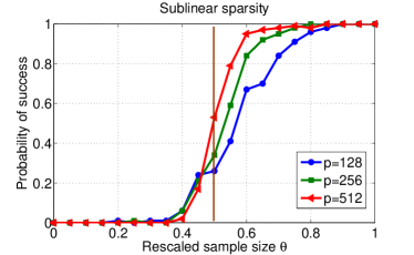
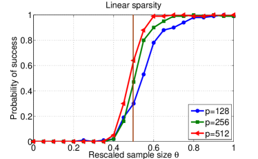
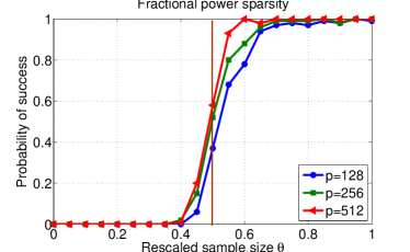
Figure 1: Probability of success in recovering the signed supports

IV Proof of Theorem 1 and related results

Proof of Theorem 1.

Since $(\widehat{\beta},\widehat{e})$ is the pair of the optimal solution of (6), we have

$$\begin{split}&\frac{1}{2n}\left\|y-X\widehat{\beta}-\sqrt{n}\widehat{e}\right\|_{2}^{2}+\lambda_{n,\beta}\left\|\widehat{\beta}\right\|_{1}+\lambda_{n,e}\left\|\widehat{e}\right\|_{1}\\ &\leq\frac{1}{2n}\left\|y-X\beta^{\star}-\sqrt{n}e^{\star}\right\|_{2}^{2}+\lambda_{n,\beta}\left\|\beta^{\star}\right\|_{1}+\lambda_{n,e}\left\|e^{\star}\right\|_{1}.\end{split}$$ (23)

From $h=\widehat{\beta}-\beta^{\star}$ and $f=\widehat{e}-e^{\star}$, we can easily see that

$$\left\|y-X\widehat{\beta}-\sqrt{n}\widehat{e}\right\|_{2}^{2} =\left\|y-X\beta^{\star}-\sqrt{n}e^{\star}\right\|_{2}^{2}$$

$$-2\left<w,Xh+\sqrt{n}f\right>+\left\|Xh+\sqrt{n}f\right\|_{2}^{2}.$$

Moreover, it is clear that

$$\begin{split}\left\|\beta^{\star}\right\|_{1}-\left\|\widehat{\beta}\right\|_{1}&=\left\|\beta^{\star}\right\|_{1}-\left\|\beta^{\star}+h\right\|_{1}\\ &=\left\|\beta^{\star}\right\|_{1}-\left\|\beta^{\star}+h_{T}\right\|_{1}-\left\|h_{T^{c}}\right\|_{1}\\ &\leq\left\|h_{T}\right\|_{1}-\left\|h_{T^{c}}\right\|_{1}.\end{split}$$

We also have a similar bound with $e$

$$\left\|e^{\star}\right\|_{1}-\left\|\widehat{e}\right\|_{1}\leq\left\|f_{S}\right\|_{1}-\left\|f_{S^{c}}\right\|_{1}.$$

Putting these pieces into (LABEL:inq::inequality_of_optimal_solution_-_1st) we can bound

$$\begin{split}&\frac{1}{2n}\left\|Xh+\sqrt{n}f\right\|_{2}^{2}\\ &\leq\frac{1}{n}\left<w,Xh+\sqrt{n}f\right>+\lambda_{n,\beta}(\left\|h_{T}\right\|_{1}-\left\|h_{T^{c}}\right\|_{1})\\ &+\lambda_{n,e}(\left\|f_{S}\right\|_{1}-\left\|f_{S^{c}}\right\|_{1})\\ &\leq\frac{1}{n}\left\|X^{*}w\right\|_{\infty}\left\|h\right\|_{1}+\frac{1}{\sqrt{n}}\left\|w\right\|_{\infty}\left\|f\right\|_{1}\\ &+\lambda_{n,\beta}(\left\|h_{T}\right\|_{1}-\left\|h_{T^{c}}\right\|_{1})+\lambda_{n,e}(\left\|f_{S}\right\|_{1}-\left\|f_{S^{c}}\right\|_{1})\\ &\leq\left(\frac{1}{n}\left\|X^{*}w\right\|_{\infty}+\lambda_{n,\beta}\right)\left\|h_{T}\right\|_{1}-\left(\lambda_{n,\beta}-\frac{1}{n}\left\|X^{*}w\right\|_{\infty}\right)\left\|h_{T^{c}}\right\|_{1}\\ &{}+\left(\frac{1}{\sqrt{n}}\left\|w\right\|_{\infty}+\lambda_{n,e}\right)\left\|f_{S}\right\|_{1}-\left(\lambda_{n,e}-\frac{1}{\sqrt{n}}\left\|w\right\|_{\infty}\right)\left\|f_{S^{c}}\right\|_{1}.\end{split}$$ (24)

By the choices of $\lambda_{n,\beta}$ and $\lambda_{n,e}$ in the lemma, we have $\frac{1}{n}\left\|X^{*}w\right\|_{\infty}\leq\frac{\gamma}{2}\lambda_{n,\beta}\leq\frac{\lambda_{n,\beta}}{2}$ and $\frac{1}{\sqrt{n}}\left\|w\right\|_{\infty}\leq\frac{\lambda_{n,e}}{2}$. Therefore,

$$\frac{1}{2n}\left\|Xh+\sqrt{n}f\right\|_{2}^{2} \leq\lambda_{n,\beta}\frac{3}{2}\left\|h_{T}\right\|_{1}-\frac{\lambda_{n,\beta}}{2}\left\|h_{T^{c}}\right\|_{1}$$

$$+\frac{3}{2}\lambda_{n,e}\left\|f_{S}\right\|_{1}-\frac{1}{2}\lambda_{n,e}\left\|f_{S^{c}}\right\|_{1}.$$

The left-hand side is greater than zero, thus the error pair $(h,f)$ belongs to the set $\mathbb{C}$ defined in (11). Hence, by the extended RE,

$$\kappa^{2}_{l}(\left\|h\right\|_{2}+\left\|f\right\|_{2})^{2} \leq 3\lambda_{n,\beta}\left\|h_{T}\right\|_{1}+3\lambda_{n,e}\left\|f_{S}\right\|_{1}$$

$$\leq 3\lambda_{n,\beta}\sqrt{k}\left\|h\right\|_{2}+\lambda_{n,e}\sqrt{s}\left\|f\right\|_{2},$$

where the last inequality follows from the crude $\ell_{1}/\ell_{2}$ bound: $\left\|h_{T}\right\|_{1}\leq\sqrt{k}\left\|h\right\|_{2}$. If $\lambda\sqrt{s/k}\leq 1$, the right-hand side is upper bounded by $3\lambda_{n,\beta}\sqrt{k}(\left\|h\right\|_{2}+\left\|f\right\|_{2})$. On the other hand, it is upper bounded by $3\lambda_{n,e}\sqrt{s}(\left\|h\right\|_{2}+\left\|f\right\|_{2})$ if $\lambda\sqrt{s/k}\geq 1$. Combining these pieces together, we conclude

$$\left\|h\right\|_{2}+\left\|f\right\|_{2}\leq 3\kappa_{l}^{-2}\max\left\{\lambda_{n,\beta}\sqrt{k},\lambda_{n,e}\sqrt{s}\right\},$$

which completes our proof. ∎

Proof of Lemma 1.

Decompose $\frac{1}{n}\left\|Xh+\sqrt{n}f\right\|_{2}^{2}=\frac{1}{n}\left\|Xh\right\|_{2}^{2}+\left\|f\right\|_{2}^{2}+\frac{2}{\sqrt{n}}\left<Xh,f\right>$. In order to lower bound the left-hand side, our main tool is to control the lower bound of each term on the right-hand side.

To establish a lower bound of $\frac{1}{n}\left\|Xh\right\|_{2}^{2}$, we leverage an appealing result of [33]. This result stated that for any Gaussian random matrix $X$ with i.i.d. $\mathcal{N}(0,\Sigma)$ rows, there exists universal positive constants $c_{1},c_{2}$ such that the following inequality holds with probability greater than $1-c_{1}\exp(-c_{2}n)$

$$\frac{1}{\sqrt{n}}\left\|Xv\right\|_{2}\geq\frac{\sqrt{C_{\min}}}{4}\left\|v\right\|_{2}-9\sqrt{\xi(\Sigma)}\sqrt{\frac{\log p}{n}}\left\|v\right\|_{1}$$ (25)

for $\forall v\in\mathbb{R}^{p}$. Here, we remind the reader of the notation $\xi(\Sigma)=\max_{j=1,...,d}\Sigma_{jj}$ and $C_{\min}=\lambda_{\min}(\Sigma)$.

We now apply this inequality for the error vector $h$ in the set $\mathbb{C}$. Since $h\in\mathbb{C}$, we have

$$\left\|h\right\|_{1} \leq 4\left\|h_{T}\right\|_{1}+3\lambda\left\|f_{S}\right\|_{1}\leq 4\sqrt{k}\left\|h\right\|_{2}+3\lambda\sqrt{s}\left\|f\right\|_{2}.$$

Next taking advantage of (25) yields

$$\frac{1}{\sqrt{n}}\left\|Xh\right\|_{2} \geq\left(\frac{\sqrt{C_{\min}}}{4}-36\sqrt{\frac{\xi k\log p}{n}}\right)\left\|h\right\|_{2}$$

$$-27\lambda\sqrt{\frac{\xi s\log p}{n}}\left\|f\right\|_{2}.$$

where we denote the shorthand notation $\xi:=\xi(\Sigma)$. This inequality leads to

$$\frac{1}{\sqrt{n}}\left\|Xh\right\|_{2}+\left\|f\right\|_{2} \geq\left(\frac{\sqrt{C_{\min}}}{4}-36\sqrt{\frac{\xi k\log p}{n}}\right)\left\|h\right\|_{2}$$

$$+\left(1-27\lambda\sqrt{\frac{\xi s\log p}{n}}\right)\left\|f\right\|_{2}.$$

From the assumptions of the lemma and the choice of $\lambda$ in (14), the two quantities in the brackets are strictly greater than $0$. Thus, $\frac{1}{\sqrt{n}}\left\|Xh\right\|_{2}+\left\|f\right\|_{2}\geq\frac{1}{2}(\left\|h\right\|_{2}+\left\|f\right\|_{2})$; or equivalent $\frac{1}{n}\left\|Xh\right\|^{2}_{2}+\left\|f\right\|^{2}_{2}\geq\frac{1}{8}(\left\|h\right\|_{2}^{2}+\left\|f\right\|_{2}^{2})$.

In combination with the following lemma 2, we conclude that

$$\frac{1}{n}\left\|Xh+\sqrt{n}f\right\|^{2}_{2}\geq\frac{1}{16}(\left\|h\right\|_{2}^{2}+\left\|f\right\|_{2}^{2}),$$

as claimed. ∎

Lemma 2.

Consider the random Gaussian design matrix $X$ whose rows are i.i.d. $\mathcal{N}(0,\Sigma)$. Assume that $n^{2}C_{\max}\xi(\Sigma)=\Theta(1)$. Suppose that $s\leq C_{1}\frac{k\log p}{\gamma\log n}$ and $n\geq C_{2}k\log p$, then the following inequality holds with probability greater than $1-\exp(-cn)$

$$\frac{2}{\sqrt{n}}|\left<Xh,f\right>|\leq\frac{1}{16}(\left\|h\right\|_{2}^{2}+\left\|f\right\|_{2}^{2}).$$

Proof.

Divide the set $T^{c}$ into subset $T_{1},T_{2},...,T_{q}$ of size $k$ such that the first set $T_{1}$ contains $k$ entries of $h$ indexed by $T$, the set $T_{2}$ contains $k$ largest absolute entries of the vector $h_{T^{c}}$, $T_{3}$ contains the second $k$ largest absolution entries of $h_{T^{c}}$ and so on. By the same strategy, we also divide the set $S^{c}$ into subset $S_{1},S_{2},...,S_{r}$ such that the first set $S_{1}$ contains $s$ entries of $f$ indexed by $S$ and sets $S_{2},S_{3},...$ are of size $s^{\prime}\geq s$.

We now have

$$\frac{1}{\sqrt{n}}|\left<Xh,f\right>| \leq\sum_{i,j}\frac{1}{\sqrt{n}}|\left<X_{S_{i}T_{j}}h_{T_{j}},f_{S_{i}}\right>|$$

$$\leq\max_{ij}\frac{1}{\sqrt{n}}\left\|X_{S_{i}T_{j}}\right\|\sum_{ij}\left\|h_{T_{j}}\right\|_{2}\left\|f_{S_{i}}\right\|_{2}.$$

Notice that the matrix $X_{S_{i}T_{j}}$ is the random Gaussian matrix whose rows are $\mathcal{N}(0,\Sigma_{T_{j}T_{j}})$. By the random Gaussian matrix concentration in Lemma 14 in Appendix VIII-D, we have with probability greater than $1-2\exp(-\tau^{2}n/2)$,

$$\frac{1}{\sqrt{n}}\left\|X_{S_{i}T_{j}}\right\|\leq\left\|\Sigma^{1/2}_{T_{j}T_{j}}\right\|\left(\sqrt{\frac{k}{n}}+\sqrt{\frac{s^{\prime}}{n}}+\tau\right).$$

Taking the union bound over all possibility of $T_{j}$ and $S_{i}$, we have this inequality holds with probability at least $1-2\binom{n}{s}\binom{p}{k}\exp(-\tau^{2}n/2)$. Assuming that $n\geq c^{-1}_{1}k\log(p/k)$, we have $\binom{p}{k}\leq\left(\frac{ep}{k}\right)^{k}\leq\exp(c_{1}n)$. In addition, assuming $n\geq c^{-1}_{2}s^{\prime}\log(n/s^{\prime})$, we have $\binom{n}{s^{\prime}}\leq\left(\frac{en}{s^{\prime}}\right)^{s}\leq\exp(c_{2}n)$. Therefore, with sufficiently small constants $c_{1}$ and $c_{2}$, we get

$$\max_{ij}\frac{1}{\sqrt{n}}\left\|X_{S_{i}T_{j}}\right\|\leq\sqrt{C_{\max}}\left(\sqrt{\frac{k}{n}}+\sqrt{\frac{s^{\prime}}{n}}+\tau\right).$$

with probability at least $1-\exp(-(\tau^{2}/2-c_{1}-c_{2})n)$ where we recall the definition of $C_{\max}:=\lambda_{\max}(\Sigma)$.

A standard bound in [36] gives us: $\sum_{i=3}^{q}\left\|h_{T_{i}}\right\|_{2}\leq k^{-1/2}\left\|h_{T^{c}}\right\|_{1}$. In addition, since $h$ belongs to the set $\mathbb{C}$, $\left\|h_{T^{c}}\right\|_{1}\leq 3\sqrt{k}\left\|h\right\|_{2}+3\lambda\sqrt{s}\left\|f\right\|_{2}$. Hence,

$$\sum_{i=1}^{q}\left\|h_{T_{i}}\right\|_{2} \leq 2\left\|h\right\|_{2}+\sum_{i=3}^{q}\left\|h_{T_{i}}\right\|_{2}\leq 5\left\|h\right\|_{2}+3\lambda\sqrt{\frac{s}{k}}\left\|f\right\|_{2}.$$

Similar manipulations along with the choice of $s^{\prime}\geq s$ also yields

$$\sum_{i=3}^{r}\left\|f_{S_{i}}\right\|_{2}\leq s^{\prime-1/2}\left\|f_{S^{c}}\right\|_{1}\leq\frac{3}{\lambda}\sqrt{\frac{k}{s^{\prime}}}\left\|h\right\|_{2}+3\left\|f\right\|_{2},$$

leading to

$$\sum_{i=1}^{r}\left\|f_{S_{i}}\right\|_{2}\leq\frac{3}{\lambda}\sqrt{\frac{k}{s^{\prime}}}\left\|h\right\|_{2}+5\left\|f\right\|_{2}.$$

Hence, $\frac{1}{\sqrt{n}}|\left<Xh,f\right>|$ is upper bounded by

$$C^{1/2}_{\max}\left(\sqrt{\frac{k}{n}}+\sqrt{\frac{s^{\prime}}{n}}+\tau\right)$$

$$\times\left(5\left\|h\right\|_{2}+3\lambda\sqrt{\frac{s^{\prime}}{k}}\left\|f\right\|_{2}\right)\left(\frac{3}{\lambda}\sqrt{\frac{k}{s^{\prime}}}\left\|h\right\|_{2}+5\left\|f\right\|_{2}\right)$$

$$\leq 25C^{1/2}_{\max}\left(\sqrt{\frac{k}{n}}+\sqrt{\frac{s^{\prime}}{n}}+\tau\right)$$

$$\times\max\left\{\lambda\sqrt{\frac{s^{\prime}}{k}},\frac{1}{\lambda}\sqrt{\frac{k}{s^{\prime}}}\right\}(\left\|h\right\|_{2}+\left\|f\right\|_{2})^{2}.$$

We select $s^{\prime}=C\frac{k\log p}{\gamma^{2}\log n}$ with an appropriate constant $C$. From the assumption that $C_{\max}\xi(\Sigma)=\Theta(1)$ and a few algebraic manipulations, we can show that $25C^{1/2}_{\max}\max\left\{\lambda\sqrt{\frac{s^{\prime}}{k}},\frac{1}{\lambda}\sqrt{\frac{k}{s^{\prime}}}\right\}\leq c\frac{1}{\sqrt{n}}$. Therefore,

$$\frac{1}{\sqrt{n}}|\left<Xh,f\right>| \leq c\left(\sqrt{\frac{k}{n}}+\sqrt{\frac{s^{\prime}}{n}}+\tau\right)(\left\|h\right\|_{2}+\left\|f\right\|_{2})^{2}$$

$$\leq\frac{1}{16}(\left\|h\right\|_{2}+\left\|f\right\|_{2})^{2}$$

for sufficiently small $\tau$ and $n\geq Cs^{\prime}$. ∎

V Proof of Theorem 2 - Achievability

By KKT condition, $\widehat{\beta}$ and $\widehat{e}$ is a pair of solution of (6) if and only if the following set of equations satisfies

$$-\frac{1}{n}X^{*}(y-X\widehat{\beta}-\widehat{e})+\lambda_{n,\beta}z^{(\beta)} = 0$$ (26)

$$-\frac{1}{\sqrt{n}}(y-X\widehat{\beta}-\widehat{e})+\lambda_{n,e}z^{(e)} = 0,$$ (27)

where $z^{(\beta)}$ and $z^{(e)}$ are elements of the subgradients of the $\ell_{1}$ norm evaluated at $\widehat{\beta}$ and $\widehat{e}$, respectively. It has been well established that $(\widehat{\beta},\widehat{e})$ is the unique solution to the extended Lasso program if

$$\begin{cases}\frac{1}{n}X^{*}_{i}(y-X\widehat{\beta}-\widehat{e})=\lambda_{n,\beta}\operatorname*{sgn}(\widehat{\beta}_{i})\quad&\text{for }\widehat{\beta}_{i}\neq 0\\ |z^{(\beta)}_{i}|=\frac{1}{n\lambda_{n,\beta}}|X^{*}_{i}(y-X\widehat{\beta}-\widehat{e})|<1\quad&\text{for }\widehat{\beta}_{i}=0.\\ \end{cases}$$ (28)

and

$$\begin{cases}\frac{1}{\sqrt{n}}(y_{i}-X_{i}\widehat{\beta}-\widehat{e}_{i})=\lambda_{n,e}\operatorname*{sgn}(\widehat{e}_{i})\quad&\text{for }\widehat{e}_{i}\neq 0\\ |z^{(e)}_{i}|=\frac{1}{\sqrt{n}\lambda_{n,e}}|y_{i}-X_{i}\widehat{\beta}-\widehat{e}_{i}|<1\quad&\text{for }\widehat{e}_{i}=0,\\ \end{cases}$$ (29)

We will show that under the assumptions of Theorem 2, the solution pair of the extended Lasso is given by $(\widehat{\beta},\widehat{e})=(\beta^{\star}+h,e^{\star}+g)$ where $h_{T^{c}}=0$, $g_{S^{c}}=0$ and

$$\begin{split}h_{T}&=(X^{*}_{S^{c}T}X_{S^{c}T})^{-1}\\ &\times[X^{*}_{S^{c}T}w_{S^{c}}+\sqrt{n}\lambda_{n,e}X^{*}_{ST}\operatorname*{sgn}(e^{\star}_{S})-n\lambda_{n,\beta}\operatorname*{sgn}(\beta^{\star}_{T})],\end{split}$$ (30)

and

$$\begin{split}g_{S}&=-\frac{1}{\sqrt{n}}X_{ST}(X^{*}_{S^{c}T}X_{S^{c}T})^{-1}\\ &\times[X^{*}_{S^{c}T}w_{S^{c}}+\sqrt{n}\lambda_{n,e}X^{*}_{ST}\operatorname*{sgn}(e^{\star}_{S})-n\lambda_{n,\beta}\operatorname*{sgn}(\beta^{\star}_{T})]\\ &+\frac{1}{\sqrt{n}}w_{S}-\lambda_{n,e}\operatorname*{sgn}(e^{\star}_{S}).\end{split}$$ (31)

The expressions of $h_{T}$ and $g_{S}$ in the above equations are obtained by solving the KKT conditions (26) and (27) restricted on $\widehat{\beta}_{T^{c}}=0$ and $\widehat{e}_{S^{c}}=0$ together with setting $z^{(\beta)}_{T}=\operatorname*{sgn}(\beta^{\star}_{T})$ and $z^{(e)}_{S}=\operatorname*{sgn}(e^{\star}_{S})$. We note that due to the conditions of the sample size $n$ and the fraction of errors in Theorem 2, $X^{*}_{S^{c}T}X_{S^{c}T}$ is invertible thanks to the random Gaussian matrix concentration inequalities (see Lemma 14 in Appendix VIII-D). Therefore, the expressions of $h_{T}$ and $g_{S}$ are valid.

To confirm that $(\widehat{\beta},\widehat{e})$ is the optimal solution of the extended Lasso (6), in the following subsections, we will check that $\widehat{\beta}$ and $\widehat{e}$ chosen above obey conditions (28) and (29). In particular,

1. In Subsection V-A, we show that $\left\|z^{(\beta)}_{T^{c}}\right\|_{\infty}<1$.

2. In Subsection V-B, we show that $\left\|z^{(e)}_{S^{c}}\right\|_{\infty}<1$.

3. In Subsection V-C, we establish that $\left\|h_{T}\right\|_{\infty}\leq f_{\beta}(\lambda_{n,\beta})$. It then follows from the assumptions of Theorem 2 that $\left\|h_{T}\right\|_{\infty}<\min_{i\in T}|\beta^{\star}_{i}|$ and, therefore, $\text{supp}(\widehat{\beta}_{T})=\text{supp}(\beta^{\star}_{T})$ and $\operatorname*{sgn}(\widehat{\beta}_{T})=\operatorname*{sgn}(\beta^{\star}_{T})$.

4. In Subsection V-D, we establish that $\left\|g_{S}\right\|_{\infty}\leq f_{e}(\lambda_{n,\beta},\lambda_{n,e})$. It then follows from the assumptions Theorem 2 that $\left\|g_{S}\right\|_{\infty}<\min_{i\in S}|e^{\star}_{i}|$ and, therefore, $\text{supp}(\widehat{e}_{S})=\text{supp}(e^{\star}_{S})$ and $\operatorname*{sgn}(\widehat{e}_{S})=\operatorname*{sgn}(e^{\star}_{S})$.

V-A Verify the upper bound of $\left\|z^{(\beta)}_{T^{c}}\right\|_{\infty}$

Proof.

First, we define a notation which will be used throughout the rest of the paper. Let $\lambda:=\frac{\lambda_{n,e}}{\lambda_{n,\beta}}$. By the definition of $\lambda_{n,\beta}$ and $\lambda_{n,e}$ in (19), we have

$$\lambda=\frac{\gamma}{2\sqrt{\max\{\rho_{u},D^{+}_{\max}\}}}\sqrt{\frac{1}{\eta\log p}},$$ (32)

where we introduce another shorthand notation $\rho_{u}=\rho_{u}(\Sigma_{T^{c}|T})$.

From the expression of $\widehat{\beta}=\beta^{\star}+h$ and $\widehat{e}=e^{\star}+g$ with $h_{T^{c}}=0$, $g_{S^{c}}=0$ and $h_{T}$, $g_{S}$ defined in (30) and (31), we substitute into $z^{(\beta)}_{T^{c}}=\frac{1}{\lambda_{n,\beta}}X^{*}_{T^{c}}(y-X\widehat{\beta}-\widehat{e})$ together with noticing that $X^{*}_{T^{c}}X_{T}-X^{*}_{ST^{c}}X_{ST}=X^{*}_{S^{c}T^{c}}X_{S^{c}T}$, $X^{*}_{T^{c}}w-X^{*}_{ST^{c}}w_{S}=X^{*}_{S^{c}T^{c}}w_{S^{c}}$ to arrive at

$$\begin{split}z^{(\beta)}_{T^{c}}&=\frac{1}{n\lambda_{n,\beta}}X^{*}_{S^{c}T^{c}}\Pi_{S^{c}T}w_{S^{c}}\\ &{}-X^{*}_{S^{c}T^{c}}X_{S^{c}T}(X^{*}_{S^{c}T}X_{S^{c}T})^{-1}z\\ &{}+\frac{1}{\sqrt{n}}\lambda X^{*}_{ST^{c}}\operatorname*{sgn}(e^{\star}_{S}).\end{split}$$ (33)

Here, we define $\Pi_{S^{c}T}:=I-X_{S^{c}T}(X^{*}_{S^{c}T}X_{S^{c}T})^{-1}X^{*}_{S^{c}T}$ which is an orthogonal projection onto the column space of $X_{S^{c}T}$ and $z:=\frac{1}{\sqrt{n}}\lambda X^{*}_{ST}\operatorname*{sgn}(e^{\star}_{S})-\operatorname*{sgn}(\beta^{\star}_{T})$.

We can further simplify the expression of $z^{(\beta)}_{T^{c}}$ by denoting

$$v:=\left(\begin{array}[]{c}\frac{1}{\sqrt{n}}\lambda\operatorname*{sgn}(e^{\star}_{S})\\ \frac{1}{n\lambda_{n,\beta}}\Pi_{S^{c}T}w_{S^{c}}-X_{S^{c}T}(X^{*}_{S^{c}T}X_{S^{c}T})^{-1}z\\ \end{array}\right),$$ (34)

then we have

$$z^{(\beta)}_{T^{c}}=[X^{*}_{ST^{c}}\quad X^{*}_{S^{c}T^{c}}]v=X^{*}_{T^{c}}v.$$ (35)

Conditioning on $X_{T}$, the matrix $X^{*}_{T^{c}}$ can be decomposed into a linear prediction plus a prediction error

$$X^{*}_{T^{c}}=\Sigma_{T^{c}T}\Sigma^{-1}_{TT}X^{*}_{T}+E^{*}_{T^{c}},$$ (36)

where each row of the matrix $E_{S^{c}T^{c}}$ is a $\mathcal{N}(0,\Sigma_{T^{c}|T})$ Gaussian random vector whose entries are i.i.d and $\Sigma_{T^{c}|T}$ is defined in (18). Therefore, $z^{(\beta)}_{T^{c}}$ consists of two components in which the first is

$$a:=\Sigma_{T^{c}T}\Sigma^{-1}_{TT}X^{*}_{T}v,$$

and the second is

$$b:=E^{*}_{T^{c}}v.$$ (37)

Since $\Pi_{S^{c}T}$ is the orthogonal projection onto the space spanned by columns of the matrix $X_{S^{c}T}$, we have $X^{*}_{S^{c}T}\Pi_{S^{c}T}=0$. Thus, $a$ can be simplified as

$$\begin{split}a&=\frac{1}{\sqrt{n}}\Sigma_{T^{c}T}\Sigma^{-1}_{TT}(\lambda X^{*}_{ST}\operatorname*{sgn}(e^{\star}_{S}))-\Sigma_{T^{c}T}\Sigma^{-1}_{TT}z\\ &=\Sigma_{T^{c}T}\Sigma^{-1}_{TT}\operatorname*{sgn}(\beta^{\star}_{T}).\end{split}$$ (38)

The mutual incoherent assumption in (17) gives us $\left\|a\right\|_{\infty}\leq 1-\gamma$. All that left is to establish the $\ell_{\infty}$-norm of the second component: $\left\|b\right\|_{\infty}\leq\gamma$. Denote $E_{i}$ as the $i$-th column of the matrix $E_{T^{c}}$ and condition on $X_{S^{c}T}$, the $i$-th coefficient of the vector $b$: $b_{i}=\left<E_{i},v\right>$ is a Gaussian random variable with variance $\operatorname*{Var}(b_{i}):=v^{*}\mathbb{E}E_{i}E_{i}^{*}v\leq\rho_{u}\left\|v\right\|_{2}^{2}$ where $\left\|v\right\|_{2}^{2}$ is quantified as,

$$M:=\frac{\lambda^{2}s}{n}+\frac{1}{n^{2}\lambda_{n,\beta}^{2}}\left\|\Pi_{S^{c}T}w_{S^{c}}\right\|_{2}^{2}+z^{*}(X_{S^{c}T}^{*}X_{S^{c}T})^{-1}z.$$ (39)

We state two supporting lemmas whose proof are deferred to the end of this section.

Lemma 3.

Denote $z=\frac{1}{\sqrt{n}}\lambda X^{*}_{ST}\operatorname*{sgn}(e_{S}^{\star})-\operatorname*{sgn}(\beta_{T}^{\star})$. Define the event

$$\mathcal{E}_{z}:=\left\{\left\|z\right\|_{\infty}\leq\lambda\sqrt{\frac{D^{+}_{\max}s\log p}{n}}+1\right\}.$$

Then, $\mathbb{P}(\mathcal{E}_{z})\geq 1-2\exp(-\log p)$.

Lemma 4.

For any $\epsilon\in(0,1)$, define the event $\overline{\mathcal{E}}=\{M\leq\overline{M}\}$, where

$$\begin{split}\overline{M}&:=\frac{1}{n}\lambda^{2}s+\left(1+\max\left\{\epsilon,4\sqrt{\frac{k}{n-s}}\right\}\right)\\ &\times\left(\frac{\sigma^{2}(n-s)}{n^{2}\lambda_{n,\beta}^{2}}+\frac{k\left(1+\lambda\sqrt{\frac{D^{+}_{\max}s\log p}{n}}\right)^{2}}{(n-s)C_{\min}}\right).\end{split}$$ (40)

Then, $\mathbb{P}(\overline{\mathcal{E}})\geq 1-c_{1}\exp(-c_{2}(n-s)\epsilon^{2}\})$ for some universal constants $c_{1},c_{2}>0$.

Conditioned on the event $\overline{\mathcal{E}}$ defined in Lemma 4, the probability $\mathbb{P}(\max_{i\in T^{c}}|b_{i}|\geq\gamma)$ is upper bounded by

$$\mathbb{P}(\max_{i\in T^{c}}|b_{i}|\geq\gamma\text{ }|\text{ }\overline{\mathcal{E}})+\exp(-c_{2}(n-s)).$$

We recall that $b_{i}$ is a zero-mean Gaussian random variable, thus the standard Gaussian tail bound in (61) allows us to derive

$$\mathbb{P}(\max_{i\in T^{c}}|b_{i}|\geq\gamma\text{ }|\text{ }\overline{\mathcal{E}})\leq 2(p-k)\exp\left(-\frac{\gamma^{2}}{2\rho_{u}\overline{M}}\right).$$

This exponential probability decays at the rate of $\exp(-c\log(p-k))$ provided that $\frac{1}{\gamma^{2}}2\rho_{u}\overline{M}\log(p-k)$ is strictly less than one. Now we replace the definition of $\overline{M}$ in (40) into this inequality. To do this, we notice that $\frac{k}{n-s}=o(1)$ from the sample size assumption of Theorem 2, thus we can select $\epsilon\in(0,1)$ such that $4\sqrt{\frac{k}{n-s}}\leq\epsilon$. Following some simple algebra, we find that it is sufficient to have

$$\frac{n-s}{1+\epsilon}>\frac{2\rho_{u}}{C_{\min}\gamma^{2}}k\log(p-k)\times\left\{\frac{C_{\min}(n-s)}{(1+\epsilon)k}\frac{\lambda^{2}s}{n}\right.\\ \left.+\left(1+\lambda\sqrt{\frac{D^{+}_{\max}s\log p}{n}}\right)^{2}+\frac{(n-s)^{2}}{n^{2}}\frac{\sigma^{2}C_{\min}}{\lambda_{n,\beta}^{2}k}\right\}.$$

Replace the expression of $\lambda$ in (32) and $s=\eta n$ and perform some simple algebra, we conclude that the $\ell_{\infty}$-norm of $z^{(\beta)}_{T^{c}}$ is strictly less than one as long as the following bound of the sample size obeys

$$\frac{n}{2(1+\epsilon)}>\frac{1}{(1-\eta)} \frac{2\rho_{u}}{C_{\min}\gamma^{2}}k\log(p-k)$$

$$\times\left\{\frac{9}{4}+(1-\eta)^{2}\frac{\sigma^{2}C_{\min}}{\lambda_{n,\beta}^{2}k}\right\},$$

which matches with the assumption of Theorem 2. ∎

Proof of Lemma 3.

Recall the expression of $z$ in the lemma, we have by the triangular inequality, $\left\|z\right\|_{\infty}\leq\frac{\lambda}{\sqrt{n}}\left\|X^{*}_{ST}\operatorname*{sgn}(e^{\star}_{S})\right\|_{\infty}+1$. Furthermore, we know that the matrix $X_{ST}$ can be represented as $W_{ST}\Sigma_{TT}^{1/2}$ where $W_{ST}\in\mathbb{R}^{s\times k}$ is the random matrix with i.i.d. zero mean entries and unit variance. Hence,

$$\left\|X^{*}_{ST}\operatorname*{sgn}(e^{\star}_{S})\right\|_{\infty} =\left\|\Sigma^{1/2}_{TT}W^{*}_{ST}\operatorname*{sgn}(e^{\star}_{S})\right\|_{\infty}$$

$$\leq\sqrt{D^{+}_{\max}}\left\|W^{*}_{ST}\operatorname*{sgn}(e^{\star}_{S})\right\|_{\infty},$$

where the inequality follows from matrix sub-multiplicative norm and $\left\|\Sigma^{1/2}_{TT}\right\|_{\infty}\leq\left\|\Sigma_{TT}\right\|^{1/2}_{\infty}=\sqrt{D^{+}_{\max}}$.

Consider the random variable $V_{i}=\left<w_{i},\operatorname*{sgn}(e^{\star}_{S})\right>$ where $w_{i}$ is a column vector of $W_{ST}$. Recall that each entry of $w_{i}$ is $\mathcal{N}(0,1)$ and $\left\|\operatorname*{sgn}(e^{\star}_{S})\right\|_{2}=\sqrt{s}$. Hence, $V_{i}$ is a Gaussian r.v. with variance $s$. Applying Gaussian tail bound (61) in the Appendix together with taking the union bound yields

$$\mathbb{P}\left(\left\|W^{*}_{ST}\operatorname*{sgn}(e^{\star}_{S})\right\|_{\infty}\geq\tau\right)\leq 2k\exp(-\tau^{2}/2s).$$

Selecting $\tau=2\sqrt{s\log p}$ so that the probability exponentially decays to zero. Combining these inequalities completes the proof of Lemma 3. ∎

Proof of Lemma 4.

Since $\Pi_{S^{c}T}$ is the orthogonal projection matrix, we have $\left\|\Pi_{S^{c}T}w_{S^{c}}\right\|_{2}^{2}\leq\left\|w_{S^{c}}\right\|_{2}^{2}$. In addition, $\frac{1}{\sigma^{2}}\left\|w_{S^{c}}\right\|_{2}^{2}$ is the $\chi^{2}$-variate with $(n-s)$ degrees of freedom, thus

$$\mathbb{P}\left(\frac{1}{n^{2}\lambda_{n,\beta}^{2}}\left\|\Pi_{S^{c}T}w_{S^{c}}\right\|_{2}^{2}\geq(1+\epsilon)\frac{\sigma^{2}(n-s)}{n^{2}\lambda_{n,\beta}^{2}}\right)\\ \leq 2\exp\left(-\frac{3(n-s)\epsilon^{2}}{16}\right).$$

Turning to the last term of $M$, by the spectral norm bound of the Gaussian random matrix (66), we obtain

$$z^{*}(X_{S^{c}T}^{*}X_{S^{c}T})^{-1}z\leq\left(1+4\sqrt{\frac{k}{n-s}}\right)\frac{\left\|z\right\|_{2}^{2}}{(n-s)C_{\min}},$$

with probability greater than $1-c_{1}\exp(-c_{2}(n-s))$. Conditioned on the event $\mathcal{E}_{z}$ in Lemma 3, we have $\left\|z\right\|_{2}^{2}\leq k\left\|z\right\|_{\infty}^{2}\leq k\left(1+\lambda\sqrt{\frac{D^{+}_{\max}s\log p}{n}}\right)^{2}$. The proof is completed by combining these bounds. ∎

V-B Verify the upper bound of $\left\|z^{(e)}_{S^{c}}\right\|_{\infty}$

Proof.

By replacing expressions of $\widehat{\beta}$ and $\widehat{e}$ into $z^{(e)}_{S^{c}}=\frac{1}{\lambda_{n,e}}(y_{S^{c}}-X_{S^{c}}\widehat{\beta})$, we get

$$\begin{split}z^{(e)}_{S^{c}}&=\frac{1}{\sqrt{n}\lambda_{n,e}}\Pi_{S^{c}T}w_{S^{c}}+\frac{\sqrt{n}}{\lambda}X_{S^{c}T}(X^{*}_{S^{c}T}X_{S^{c}T})^{-1}z,\end{split}$$ (41)

where we use the same notations of $\Pi_{S^{c}T}$ and $z$ as in the previous section: $\Pi_{S^{c}T}:=I-X_{S^{c}T}(X^{*}_{S^{c}T}X_{S^{c}T})^{-1}X^{*}_{S^{c}T}$ and $z:=\frac{1}{\sqrt{n}}\lambda X^{*}_{ST}\operatorname*{sgn}(e^{\star}_{S})-\operatorname*{sgn}(\beta^{\star}_{T})$. To show that $\left\|z^{(e)}_{S^{c}}\right\|_{\infty}<1$, we bound $\ell_{\infty}$-norm of each term of the sum (41) separately. In particular, we will establish that with probability converging to one, the $\ell_{\infty}$-norm of the first term is bounded by $\frac{2\sigma\sqrt{\log n}}{\lambda_{n,e}\sqrt{n}}$ and that of the second term is less than $(1-\frac{2\sigma\sqrt{\log n}}{\lambda_{n,e}\sqrt{n}})$. The proof is therefore completed by the triangular inequality.

We begin by establishing the $\ell_{\infty}$-norm of the first term of $z^{(e)}_{S^{c}}$ in (41):

$$\frac{1}{\sqrt{n}\lambda_{n,e}}\left\|\Pi_{S^{c}T}w_{S^{c}}\right\|_{\infty}=\max_{i}\frac{1}{\sqrt{n}\lambda_{n,e}}\left|\left<u_{i},w_{S^{c}}\right>\right|,$$

where $u_{i}$ is a column vector of $\Pi_{S^{c}T}$. Since $\frac{1}{\sqrt{n}\lambda_{n,e}}\left<u_{i},w_{S^{c}}\right>$ is a sum of Gaussian random variables with zero mean and variance $\frac{\sigma^{2}}{n\lambda_{n,e}^{2}}\left\|u_{i}\right\|_{2}^{2}$, it can be bounded by the Gaussian tail inequality in (61) in Appendix VIII-D. Notice that spectral norm of any orthogonal projection is one, $\left\|u_{i}\right\|_{2}\leq 1$. We have

$$\mathbb{P}\left(\frac{1}{\sqrt{n}\lambda_{n,e}}\left|\left<u_{i},w_{S^{c}}\right>\right|\geq\tau\right)\leq 2\exp\left(-\frac{n\lambda^{2}_{e}\tau^{2}}{2\sigma^{2}}\right).$$

Choose $\tau=\frac{2\sigma\sqrt{\log n}}{\sqrt{n}\lambda_{n,e}}$ and take the union bound over all $|S^{c}|$ columns of the matrix $\Pi_{S^{c}T}$, we have

$$\mathbb{P}\left(\frac{1}{\sqrt{n}\lambda_{n,e}}\left\|\Pi_{S^{c}T}w_{S^{c}}\right\|_{\infty}\geq\frac{2\sigma\sqrt{\log n}}{\sqrt{n}\lambda_{n,e}}\right)\\ \leq 2|S^{c}|\exp\left(-2\log n\right).$$ (42)

Next, we controlthe upper bound of $\frac{\sqrt{n}}{\lambda}\left\|X_{S^{c}T}(X^{*}_{S^{c}T}X_{S^{c}T})^{-1}z\right\|_{\infty}$. The following lemma, whose proof is deferred to Appendix VIII-A, establishes this bound.

Lemma 5.

Under the assumptions of Theorem 2, for any vector $z\in\mathbb{R}^{k}$ independent with $X_{S^{c}T}$, the following statement holds

$$\frac{\sqrt{n}}{\lambda}\left\|X_{S^{c}T}(X_{S^{c}T}^{*}X_{S^{c}T})^{-1}z\right\|_{\infty}<\frac{2}{3}\left(1-\frac{2\sigma\sqrt{\log n}}{\lambda_{n,e}\sqrt{n}}\right)\left\|z\right\|_{\infty}$$

with probability greater than $1-c_{1}\exp(-c_{2}\max\{\log(p-k),\log(n-s)\})$.

Since $\operatorname*{sgn}(\beta^{\star}_{T})$ and $X^{*}_{ST}\operatorname*{sgn}(e^{\star}_{S})$ are statistically independent with $X_{S^{c}T}$, $z:=\frac{1}{\sqrt{n}}\lambda X^{*}_{ST}\operatorname*{sgn}(e^{\star}_{S})-\operatorname*{sgn}(\beta^{\star}_{T})$ satisfies the assumption of Lemma 5. Moreover, by Lemma 3 and the definition of $\lambda$ in (32), we have with high probability

$$\left\|z\right\|_{\infty}\leq 1+\lambda\sqrt{\frac{D^{+}_{\max}s\log p}{n}}\leq\frac{3}{2},$$

where the last inequality holds from the assumption of Theorem 2. Now, applying Lemma 5 leads to $\frac{\sqrt{n}}{\lambda}\left\|X_{S^{c}T}(X^{*}_{S^{c}T}X_{S^{c}T})^{-1}z\right\|_{\infty}\leq 1-\frac{2\sigma\sqrt{\log n}}{\lambda_{n,e}\sqrt{n}}$.

Putting these two bounds together and using the triangular inequality we conclude that with high probability, $\left\|z^{(e)}_{S^{c}}\right\|_{\infty}<1$ as claimed. ∎

V-C Establish the $\ell_{\infty}$ bound of $\widehat{\beta}_{T}-\beta^{\star}_{T}$

Recall the formula of $(\widehat{\beta}_{T}-\beta^{\star}_{T})$ from (30), the triangular inequality yields

$$\begin{split}&\left\|\widehat{\beta}_{T}-\beta^{\star}_{T}\right\|_{\infty}\leq\left\|\left(X^{*}_{S^{c}T}X_{S^{c}T}\right)^{-1}X^{*}_{S^{c}T}w_{S^{c}}\right\|_{\infty}\\ &{}+n\lambda_{n,\beta}\left\|(X^{*}_{S^{c}T}X_{S^{c}T})^{-1}(\frac{1}{\sqrt{n}}\lambda X^{*}_{ST}\operatorname*{sgn}(e^{\star}_{S})-\operatorname*{sgn}(\beta^{\star}_{T}))\right\|_{\infty}\\ &:=\mathcal{T}_{1}+\mathcal{T}_{2}.\end{split}$$ (43)

To bound the first quantity, we consider a random vector $u=(\frac{1}{n-s}X^{*}_{S^{c}T}X_{S^{c}T})^{-1}\frac{1}{n-s}X^{*}_{S^{c}T}w_{S^{c}}$ and note that $\mathcal{T}_{1}=\left\|u\right\|_{\infty}$. This bound, which is stated below, has been established in equation (42) of [8]: there exists some numerical constant $c$ such that

$$\mathbb{P}\left(\mathcal{T}_{1}\geq 20\sqrt{\frac{\sigma^{2}\log k}{C_{\min}(n-s)}}\right)\leq 4\exp(-c(n-s)).$$ (44)

Turning now to the second quantity $\mathcal{T}_{2}$. We have

$$\mathcal{T}_{2}\leq\frac{n\lambda_{n,\beta}}{n-s}\left\|\left(\frac{X^{*}_{S^{c}T}X_{S^{c}T}}{n-s}\right)^{-1}z\right\|_{\infty},$$

where $z:=\frac{1}{\sqrt{n}}\lambda X^{*}_{ST}\operatorname*{sgn}(e^{\star}_{S})-\operatorname*{sgn}(\beta^{\star}_{T})$. To bound $\mathcal{T}_{2}$, we follow similar arguments in [8], Section V.B. We can now state the following lemma, which is modified from Lemma 5 of [8].

Lemma 6.

Let $z\in\mathbb{R}^{k}$ be a fixed nonzero vector and $W\in\mathbb{R}^{n\times k}$ be a random matrix with i.i.d entries $W_{ij}\sim\mathcal{N}(0,1)$. Then, there exists positive constants $c_{1}$ and $c_{2}$ such that

$$\begin{split}\mathbb{P}&\left(\left\|\left[\left(\frac{W^{*}W}{n}\right)^{-1}-I_{k\times k}\right]z\right\|_{\infty}\geq c_{1}\sqrt{\frac{k\log(p-k)}{n}}\left\|z\right\|_{\infty}\right)\\ &\leq 4\exp(-c_{2}\min\{k,\log(p-k)\}).\end{split}$$

Following similar arguments as in [8], Section V.B, we have a similar probabilistic bound as equation (41) of [8]

$$\mathbb{P}\left(\mathcal{T}_{2}\geq c_{1}\lambda_{n,\beta}\sqrt{\frac{kn\log(p-k)}{(n-s)^{2}}}\left\|\Sigma^{-1/2}_{TT}\right\|_{\infty}\left\|\Sigma^{-1/2}_{TT}z\right\|_{\infty}\right)\\ \leq 4\exp(-c_{2}\min\{k,\log(p-k)\}).$$ (45)

Furthermore, Lemma 3 states that $\left\|z\right\|_{\infty}\leq 3/2$ with high probability. Conditioning on the event $\mathcal{E}=\{\left\|z\right\|_{\infty}\leq 3/2\}$, we have $\left\|\Sigma^{-1/2}_{TT}z\right\|_{\infty}\leq\frac{3}{2}\left\|\Sigma^{-1/2}_{TT}\right\|_{\infty}$. Thus, (45) leads to

$$\mathbb{P}\left(\mathcal{T}_{2}\geq c_{2}\lambda_{n,\beta}\sqrt{\frac{kn\log(p-k)}{(n-s)^{2}}}\left\|\Sigma^{-1/2}_{TT}\right\|^{2}_{\infty}\text{ }|\text{ }\mathcal{E}\right)\\ \leq 4\exp(-c_{2}\min\{k,\log(p-k)\}).$$

By the total probability rule, $\mathbb{P}(\mathcal{T}_{2}\geq\tau)\leq\mathbb{P}(\mathcal{T}_{2}|\mathcal{E})+\mathbb{P}(\mathcal{E}^{c})$. Therefore, we conclude that with probability greater than $1-6\exp(-c_{2}\min\{k,\log(p-k)\})$,

$$\mathcal{T}_{2}\leq c_{2}\lambda_{n,\beta}\sqrt{\frac{k\log(p-k)}{(1-\eta)^{2}n}}\left\|\Sigma^{-1/2}_{TT}\right\|^{2}_{\infty}.$$ (46)

Overall, combining the bound of $\mathcal{T}_{2}$ with the bound of $\mathcal{T}_{1}$ in (44) concludes that $\left\|\widehat{\beta}_{T}-\beta^{\star}_{T}\right\|_{\infty}\leq f_{\beta}(\lambda_{n,\beta})$ with probability at least $1-10\exp(-c_{3}\min\{k,\log(p-k)\}$ where $f_{\beta}(\lambda_{n,\beta})$ is defined in (21).

V-D Establish the $\ell_{\infty}$ bound of $\widehat{e}_{S}-e^{\star}_{S}$

Recalling the formula of $\widehat{e}_{S}-e^{\star}_{S}$ in (31) and applying the triangular inequality, we get

$$\begin{split}\left\|\widehat{e}_{S}-e^{\star}_{S}\right\|_{\infty}&\leq\frac{1}{\sqrt{n}}\left\|X_{ST}(X^{*}_{S^{c}T}X_{S^{c}T})^{-1}X^{*}_{S^{c}T}w_{S^{c}}\right\|_{\infty}\\ &{}+\lambda_{n,\beta}\sqrt{n}\left\|X_{ST}(X^{*}_{S^{c}T}X_{S^{c}T})^{-1}z\right\|_{\infty}\\ &{}+\frac{1}{\sqrt{n}}\left\|w_{S}\right\|_{\infty}+\lambda_{n,e}\\ &:=\mathcal{T}_{1}+\mathcal{T}_{2}+\mathcal{T}_{3}+\lambda_{n,e},\end{split}$$ (47)

where we again denote $z=\frac{1}{\sqrt{n}}\lambda X^{*}_{ST}\operatorname*{sgn}(e^{\star}_{S})-\operatorname*{sgn}(\beta^{\star}_{T})$. We first consider the easiest term $\mathcal{T}_{3}=\frac{1}{\sqrt{n}}\left\|w_{S}\right\|_{\infty}$. Since $w_{S}$ is a random vector with i.i.d. $\mathcal{N}(0,\sigma^{2})$ entries, by Gaussian extreme order statistics [37], $\mathcal{T}_{3}\leq 2\sqrt{\frac{\sigma^{2}\log s}{n}}$.

Turning to the first term $\mathcal{T}_{1}$, we define a vector $v\in\mathbb{R}^{s}$ whose entries are $v_{i}:=x_{i}(X^{*}_{S^{c}T}X_{S^{c}T})^{-1}X^{*}_{S^{c}T}w_{S^{c}}$ where $x_{i}$ is the $i$-th row of the matrix $X_{ST}$ and notice that $\mathcal{T}_{1}=\left\|v\right\|_{\infty}$. Conditioned on $X_{T}$, it is clear that $v_{i}$ is a zero mean random variable with variance $\sigma^{2}x_{i}(X^{*}_{S^{c}T}X_{S^{c}T})^{-1}x^{*}_{i}$. In addition, we recall that $X_{T}$ can be represented as $X_{T}=W_{T}\Sigma^{1/2}_{TT}$ where $W_{T}$ is the $n\times k$ standard Gaussian matrix. Thus, $x_{i}(X^{*}_{S^{c}T}X_{S^{c}T})^{-1}x^{*}_{i}=w_{i}(W^{*}_{S^{c}T}W_{S^{c}T})^{-1}w^{*}_{i}\leq\left\|w_{i}\right\|_{2}^{2}\left\|(W^{*}_{S^{c}T}W_{S^{c}T})^{-1}\right\|$, where $w_{i}$ is the $i$-th row of matrix $W_{ST}$. In short, $v_{i}$ is a zero mean random variable with variance at most $\widetilde{\sigma}^{2}:=\sigma^{2}\left\|w_{i}\right\|_{2}^{2}\left\|(W^{*}_{S^{c}T}W_{S^{c}T})^{-1}\right\|$. Using the concentration result for $\chi^{2}$-variate, we get $\left\|w_{i}\right\|_{2}^{2}\leq 2k$ with probability at least $1-\exp(-k/2)$. Furthermore, from random matrix theory (65) in Appendix VIII-D, $\left\|(W^{*}_{S^{c}T}W_{S^{c}T})^{-1}\right\|\leq\frac{5}{n-s}$ with probability at least $1-\exp(-(n-s)/2)$.

Next, let us define the event

$$\mathcal{E}=\left\{\widetilde{\sigma}^{2}\geq\frac{10\sigma^{2}k}{n-s}\right\}.$$

From the above arguments, we have $\mathbb{P}(\mathcal{E})\leq\exp(-(n-s+k)/2)$. By the total probability rule, we have

$$\mathbb{P}(\mathcal{T}_{1}\geq\tau)\leq\mathbb{P}(\mathcal{T}_{1}\geq\tau|\mathcal{E}^{c})+\mathbb{P}(\mathcal{E}).$$

Conditioning on $\mathcal{E}^{c}$, $v_{i}$ is zero mean Gaussian with variance at most $\frac{10\sigma^{2}k}{n-s}$. Thus, by the Gaussian tail bound (61) in Appendix VIII-D, we derive

$$\mathbb{P}\left(\max_{i\in S}|v_{i}|\geq\tau\right)\leq 2s\exp\left(-\frac{(n-s)\tau^{2}}{10\sigma^{2}k}\right)$$

Setting $\tau=\sqrt{\frac{20\sigma^{2}k\log(p-k)}{n-s}}$ yields the fact that this probability vanishes at rate $2(p-k)^{-1}$. Overall, we can now conclude that

$$\mathbb{P}\left(\mathcal{T}_{1}\geq 11\sqrt{\frac{\sigma^{2}k\log(p-k)}{n-s}}\right)\leq 2\exp(-\log(p-k)).$$

It is left to bound $\mathcal{T}_{2}$. By sub-multiplicative norm inequality, $\mathcal{T}_{2}$ is bounded by

$$\lambda_{n,\beta}\sqrt{n}\left\|X_{ST}\right\|_{\infty}\left\|(X^{*}_{S^{c}T}X_{S^{c}T})^{-1}z\right\|_{\infty},$$

We already established $n\lambda_{n,\beta}\left\|(X^{*}_{S^{c}T}X_{S^{c}T})^{-1}z\right\|_{\infty}$ in (46). In addition, $\left\|X_{ST}\right\|_{\infty}\leq\sqrt{k}\left\|X_{ST}\right\|$ where by the matrix theory (66) in Appendix VIII-D, $\left\|X^{*}_{ST}X_{ST}\right\|\leq 4C_{\max}(s+\sqrt{sk})$ with high probability. Thus, $\left\|X_{ST}\right\|_{\infty}\leq\sqrt{C_{\max}}(sk+k\sqrt{sk})^{1/2}$.

Overall, combining with the bounds of $\mathcal{T}_{1}$ and $\mathcal{T}_{3}$, we conclude that $\left\|\widehat{\beta}_{T}-\beta^{\star}_{T}\right\|_{\infty}\leq f_{\beta}(\lambda_{n,\beta})$ with probability at least $1-10\exp(-c_{3}\min\{k,\log(p-k)\}$ where $f_{e}(\lambda_{n,\beta},\lambda_{n,e})$ is defined as in (22).

VI Proof of Theorem 3 - Inachievability

Our analysis in this section relies on the the notion of primal-dual witness introduced by Wainwright [8]. In particular, we will construct a pair of primal solutions $(\widehat{\beta},\widehat{e})$ and their dual vectors $(z^{(\beta)},z^{(e)})$. The extended Lasso (6) fails to correctly identify signed support of the coefficient vector $\beta^{\star}$ and the error $e^{\star}$ when the $\ell_{\infty}$-norm of either $z^{(\beta)}_{T^{c}}$ or $z^{(e)}_{S^{c}}$ exceeds unity with probability approaching one. The primal-dual witness is constructed as follows:

1. First, we obtain the solution pair $(\widehat{\beta}_{T},\widehat{e}_{S})$ of the following restricted Lasso problem

   $$\min_{\beta,e}\frac{1}{2n}\left\|y_{S}-X_{ST}\beta_{T}-\sqrt{n}e_{S}\right\|_{2}^{2}+\lambda_{n,\beta}\left\|\beta_{T}\right\|_{1}+\lambda_{n,e}\left\|e_{S}\right\|_{1}.$$ (48)

   We also set $\widehat{\beta}_{T^{c}}=0$ and $\widehat{e}_{S^{c}}=0$.

2. Second, we select $z^{(\beta)}_{T}$ and $z^{(e)}_{S}$ as elements of the subgradients $\left\|\widehat{\beta}\right\|_{1}$ and $\left\|\widehat{e}\right\|_{1}$, respectively.

3. Third, we solve for vectors $z^{(\beta)}_{T^{c}}$ and $z^{(e)}_{S^{c}}$ satisfying the KKT conditions in (26). We then verify whether the dual feasibility conditions of both $\left\|z^{(\beta)}_{T^{c}}\right\|_{\infty}<1$ and $\left\|\widehat{e}_{S^{c}}\right\|_{\infty}<1$ are satisfied.

4. Fourth, we check whether the sign consistency $z^{(\beta)}_{T}=\operatorname*{sgn}(\beta^{\star}_{T})$ and $z^{(e)}_{S}=\operatorname*{sgn}(e^{\star}_{S})$ are satisfied.

The following result summarizes the use of the primal-dual witness construction in providing the proof of Theorem 3:

Lemma 7.

If either steps 3 or 4 of the primal-dual construction fails, then the extended Lasso fails to recover the correct signed supports of both $\beta^{\star}$ and $e^{\star}$.

The proof of this lemma is essentially similar to that of Lemma 2(c) in [8], thus we omit the detail here.

In our proof, we assume that $z^{(\beta)}_{T}=\operatorname*{sgn}(\beta^{\star}_{T})$ and $z^{(e)}_{S}=\operatorname*{sgn}(e^{\star}_{S})$; otherwise, the sign consistency would fails. Under these assumptions, it is easy to check that the solution $(\widehat{\beta}_{T},\widehat{e}_{S})$ of the optimization (48) is expressed in (30) and (31). Thus, we can derive equations of $z^{(\beta)}_{T^{c}}$ and $z^{(e)}_{S^{c}}$ as in (33) and (41).

In the following two sections, we establish the claim by showing that under the conditions of the sample size $n$ and $s=\eta n$ as in Theorem 3, the $\ell_{\infty}$-norm of either $z^{(\beta)}_{T^{c}}$ or $z^{(e)}_{S^{c}}$ exceeds unity with probability tending to one. It is clear that if the extended Lasso (6) fails to recover signed support vectors with $s=\eta n$, it also fails to do so with $s>\eta n$ since it is easier to solve the extended Lasso when there is less corrupted observations.

VI-A Lower $\ell_{\infty}$-norm bound of $z^{(\beta)}_{T^{c}}$

Recall the expression of $z^{(\beta)}_{T^{c}}$ in (33) and its simplified form $z^{(\beta)}_{T^{c}}=a+b$ where $b$ and $a$ are defined in (37) and (38). We already have $\left\|a\right\|_{\infty}\leq 1-\gamma$ due to the mutual incoherence assumption. It is now sufficient to show that $\max_{i\in T^{c}}|b_{i}|$ exceeds $(2-\gamma)$ with high probability.

Conditioning on $X_{T}$ and $w$, the vector $b$ is zero-mean Gaussian with covariance matrix $M\Sigma_{T^{c}|T}$ where the random scaling form $M$ has the form (39). The following lemma controls the lower bound of this scaling factor. The proof is similar to that of Lemma 6 in [8], so we omit the detail here.

Lemma 8.

Define the event $\mathcal{E}=\{M>\underline{M}\}$, where $\underline{M}$ is defined in (49). Then, $\mathbb{P}(\mathcal{E})\leq 1-c_{1}\exp(-c_{2}(n-s))$ for some $c_{1},c_{2}>0$.

$$\underline{M}:=\begin{cases}\frac{\lambda^{2}s}{n}+c\frac{k}{n-s}\quad&\text{if }k/n=\Theta(1)\\ \frac{\lambda^{2}s}{n}+\left(1-\max\left\{\epsilon,4\sqrt{\frac{k}{n-s}}\right\}\right)\left(\frac{\sigma^{2}(n-s)}{n^{2}\lambda_{n,\beta}^{2}}+\frac{\left\|z\right\|_{2}^{2}}{(n-s)C_{\max}}\right)\quad&\text{if }k/n=o(1).\end{cases}$$ (49)

Following the proof of Theorem 4 in [8], we have the following lower bound: for all $\nu,\epsilon,\tau>0$

$$\max_{i\in T^{c}}|b_{i}|\geq\sqrt{(2-\nu)\rho_{l}(\Sigma_{T^{c}|T})\underline{M}\log(p-k)}-\tau$$ (50)

with probability at least $1-2\exp\left(-\frac{\tau^{2}}{2\underline{M}\rho_{u}}\right)$. Now, using appropriate choices of $\{\tau,\nu,\gamma\}$, it suffices to establish the bound

$$\rho_{l}(\Sigma_{T^{c}|T})\underline{M}\log(p-k)\geq\frac{[(2-\gamma)+\tau]^{2}}{(2-\nu)}.$$ (51)

We consider two cases:

1) If $\underline{M}\rightarrow+\infty$ or $\underline{M}=\Theta(1)$, then we can choose $\tau^{2}=\delta\underline{M}\log(p-k)$ for some $\delta>0$. For $\delta$ sufficiently small, we conclude from (50) that with probability converging to one, there exists some constants $c>0$ such that

$$\max_{i\in T^{c}}|b_{i}|\geq c\sqrt{\log(p-k)},$$

which exceeds $(2-\gamma)$ regardless of the choice of the sample size $n$.

2) Otherwise, $\underline{M}=o(1)$. This is satisfied only if $k/n=o(1)$ and thus, the second line of the definition of $\underline{M}$ is applied. Now, we can select $\tau$ sufficiently small and have a guarantee that $\frac{\tau^{2}}{2\underline{M}}\rightarrow+\infty$. From the definition of $\underline{M}$, one can see that if $\rho_{l}\frac{\lambda^{2}s}{n}\log(p-k)\geq 2$, we can choose $\tau$ and $\nu$ strictly positive but arbitrarily close to zero such that $\frac{[(2-\gamma)+\tau]^{2}}{(2-\nu)}<2$. Thus, (51) obeys regardless of the selection of the sample size $n$. Consequently, we assume that

$$\lambda<\sqrt{\frac{2n}{\rho_{l}s\log(p-k)}}.$$ (52)

Under this assumption, we can lower bound $\left\|z\right\|_{2}$ as follows

$$\begin{split}\left\|z\right\|_{2}&=\left\|\operatorname*{sgn}(\beta^{\star}_{T})-\frac{1}{\sqrt{n}}\lambda X^{*}_{ST}\operatorname*{sgn}(e^{\star}_{S})\right\|_{2}\\ &\geq\left\|\operatorname*{sgn}(\beta^{\star}_{T})\right\|_{2}-\frac{1}{\sqrt{n}}\lambda\left\|X^{*}_{ST}\operatorname*{sgn}(e^{\star}_{S})\right\|_{2}\\ &\geq\sqrt{k}-\lambda\sqrt{\frac{k}{n}}\left\|X^{*}_{ST}\operatorname*{sgn}(e^{\star}_{S})\right\|_{\infty}.\end{split}$$ (53)

As shown during the proof of Lemma 3 that $\frac{1}{\sqrt{n}}\left\|X^{*}_{ST}\operatorname*{sgn}(e^{\star}_{S})\right\|_{\infty}\leq\frac{1}{3}\sqrt{\frac{\rho_{l}s\log(p-k)}{n}}$ with probability greater than $1-\exp(-\frac{\rho_{l}}{18D^{+}_{\max}}\log p)$, from the above upper bound of $\lambda$, we obtain $\frac{\lambda}{\sqrt{n}}\left\|X^{*}_{ST}\operatorname*{sgn}(e^{\star}_{S})\right\|_{\infty}\leq\frac{\sqrt{2}}{3}$. Consequently, we achieve the lower bound with high probability

$$\left\|z\right\|_{2}\geq\frac{1}{2}\sqrt{k}.$$ (54)

Furthermore, for $(n-s)$ sufficiently large, we select a $\epsilon\in(0,1/2)$ such that $4\sqrt{\frac{k}{n-s}}<\epsilon$. Now, replace this bound into the second equation of $\underline{M}$ and perform some simple algebra, we can show that the inequality (51) is satisfied as long as

$$\frac{\rho_{l}}{C_{\max}}\frac{k\log(p-k)}{(n-s)}\left\{\frac{C_{\max}\lambda^{2}s(n-s)}{(1-\epsilon)kn}\right.\\ \left.+\frac{1}{4}+\frac{(n-s)^{2}}{n^{2}}\frac{\sigma^{2}C_{\max}}{\lambda_{n,\beta}^{2}k}\right\}\geq\frac{[(2-\gamma)+\tau]^{2}}{(2-\nu)(1-\epsilon)}.$$

Replace the lower bound of $\lambda$ in (56) and $s=\eta n$ into the above inequality, we can conclude that the inequality (51) is satisfied as long as

$$\frac{\rho_{l}}{C_{\max}(2-\gamma)^{2}} \frac{2k\log(p-k)}{(n-s)}\left\{\frac{3}{8}+(1-\eta)^{2}\frac{\sigma^{2}C_{\max}}{\lambda_{n,\beta}^{2}k}\right\}$$

$$\geq\frac{[(2-\gamma)+\tau]^{2}}{(2-\gamma)^{2}(1-\nu/2)(1-\epsilon)}.$$

Under the assumptions of Theorem 3, the right-hand side is strictly greater than one. On the other hand, $\tau,\nu$ and $\epsilon$ are parameters that can be chosen in $(0,1/2)$. By selecting these parameters to be positive but arbitrarily close to zeros, we can set the right-hand side less than one. Therefore, (51) is satisfied.

VI-B Lower the $\ell_{\infty}$-norm bound of $z^{(e)}_{S^{c}}$

Recalling the equation of $z^{(e)}_{S^{c}}$ in (41), we have

$$z^{(e)}_{S^{c}}=\frac{1}{\sqrt{n}\lambda_{n,e}}\Pi_{S^{c}T}w_{S^{c}}+\frac{\sqrt{n}}{\lambda}X_{S^{c}T}(X^{*}_{S^{c}T}X_{S^{c}T})^{-1}z$$

where we recall $z=\frac{1}{\sqrt{n}}\lambda X^{*}_{ST}\operatorname*{sgn}(e^{\star}_{S})-\operatorname*{sgn}(\beta^{\star}_{T})$. First, notice that $\Pi_{S^{c}T}$ is the orthogonal projection onto the column space of the matrix $X_{S^{c}T}$. Thus, two terms in the above summation are orthogonal to each other. Therefore, lowering the $\ell_{\infty}$-norm of $z^{(e)}_{S^{c}}$ by its $\ell_{2}$-norm counterpart, we have

$$(n-s)\left\|z^{(e)}_{S^{c}}\right\|^{2}_{\infty}\geq\left\|z^{(e)}_{S^{c}}\right\|_{2}^{2}$$

$$=\frac{1}{n\lambda_{n,e}^{2}}\left\|\Pi_{S^{c}T}w_{S^{c}}\right\|_{2}^{2}+\frac{n}{\lambda^{2}}\left\|X_{S^{c}T}(X^{*}_{S^{c}T}X_{S^{c}T})^{-1}z\right\|_{2}^{2}.$$

From this inequality, we have an important observation that both terms in the sum have to be upper bounded by $(n-s)$. Otherwise, $\left\|z^{(e)}_{S^{c}}\right\|^{2}_{\infty}$ is automatically strictly greater than one, regardless of the choice of the sample size $n$. This observation suggests to us the required lower bound of $\lambda_{n,e}$ and $\lambda$:

$$\lambda_{n,e}\geq\frac{1}{\sqrt{n(n-s)}}\left\|\Pi_{S^{c}T}w_{S^{c}}\right\|_{2},$$

and

$$\lambda\geq\sqrt{\frac{n}{n-s}}\left\|X_{S^{c}T}(X^{*}_{S^{c}T}X_{S^{c}T})^{-1}z\right\|_{2}.$$

We now explicitly establish the lower bound of these regularization parameters. First, since $\frac{1}{\sigma^{2}}\left\|\Pi_{S^{c}T}w_{S^{c}}\right\|_{2}^{2}$ is the $\chi^{2}$-variate with $n-s$ degrees of freedom, Lemma 13 in Appendix VIII-D suggests to us that $\frac{1}{\sigma^{2}}\left\|\Pi_{S^{c}T}w_{S^{c}}\right\|_{2}^{2}\geq\frac{1}{2}(n-s)$ with probability at least $1-\exp(-(n-s)/16)$. Consequently, we require

$$\lambda_{n,e}\geq\sqrt{\frac{\sigma^{2}}{2n}}.$$ (55)

Furthermore, we observe that with probability converging to one

$$\left\|X_{S^{c}T}(X^{*}_{S^{c}T}X_{S^{c}T})^{-1}z\right\|_{2}^{2} =z^{*}(X^{*}_{S^{c}T}X_{S^{c}T})^{-1}z$$

$$=z^{*}\Sigma^{-1/2}_{TT}(W^{*}_{S^{c}T}W_{S^{c}T})^{-1}\Sigma^{-1/2}_{TT}z$$

$$\geq\left\|\Sigma^{-1/2}_{TT}z\right\|^{2}_{2}\sigma_{\min}((W^{*}_{S^{c}T}W_{S^{c}T})^{-1})$$

$$\geq\frac{1}{2n}C^{-1}_{\max}\left\|z\right\|_{2}^{2},$$

where the second identity follows from the decomposition $X_{S^{c}T}=\Sigma^{1/2}_{TT}W_{S^{c}T}$ and the last inequality is due to the Gaussian random matrix inequality (63) in Appendix VIII-D. In combination with the lower bound of $\left\|z\right\|_{2}$, we require

$$\lambda\geq\sqrt{\frac{k}{8C_{\max}(n-s)}}.$$ (56)

Turning to establish the lower bound of $\left\|z^{(e)}_{S^{c}}\right\|_{\infty}$, we can show that under the assumptions of Theorem 3, this quantity is strictly greater than one. By the triangular inequality, $\left\|z^{(e)}_{S^{c}}\right\|_{\infty}\geq\mathcal{T}_{1}-\mathcal{T}_{2}$ where $\mathcal{T}_{1}$ is quantified as

$$\frac{\sqrt{n}}{\lambda}\left\|X_{S^{c}T}(X^{*}_{S^{c}T}X_{S^{c}T})^{-1}z\right\|_{\infty}$$

and the other term is $\mathcal{T}_{2}:=\frac{1}{\lambda_{n,e}\sqrt{n}}\left\|\Pi_{S^{c}T}w_{S^{c}}\right\|_{\infty}$. As shown at the beginning of Section V-B, we have the following inequality to hold with probability greater than $1-2\exp(-\log(n-s))$:

$$\mathcal{T}_{2}\leq\frac{2\sqrt{\sigma^{2}\log(n-s)}}{\lambda_{n,e}\sqrt{n}}.$$

It is now left to justify that under the assumption of Theorem 3, $\mathcal{T}_{1}>1+\frac{2\sqrt{\sigma^{2}\log n}}{\lambda_{n,e}\sqrt{n}}$. The remainder of this section is devoted to establish this claim. In what follows, we state two important lemmas, which are the main factor in establishing the lower bound of $\mathcal{T}_{1}$. The proofs of these lemmas are again deferred to the Appendix.

Lemma 9.

For any vector $z\in\mathbb{R}^{k}$ independent with $X_{S^{c}T}$, we have with probability greater than $1-\exp(-\log(n-s))$

$$\left\|X_{S^{c}T}(X^{*}_{S^{c}T}X_{S^{c}T})^{-1}z-\frac{1}{n-s}X_{S^{c}T}\Sigma^{-1}_{TT}z\right\|_{\infty}\\ \leq 16\frac{\left\|z\right\|_{2}\sqrt{2k\log(n-s)}}{\sqrt{C_{\min}(n-s)^{3}}}.$$

Lemma 10.

With probability at least $1-4\exp(-\frac{1}{4}\log(n-s))$,

$$\left\|X_{S^{c}T}\Sigma^{-1}_{TT}z\right\|_{\infty}\geq\frac{2\left\|z\right\|_{2}\sqrt{\log(n-s)}}{3\sqrt{C_{\max}}}.$$

Once these two lemmas are established, we can now show that under the assumptions of Theorem 3, $\mathcal{T}_{1}>1+\frac{\sqrt{\sigma^{2}\log n}}{\lambda_{n,e}\sqrt{n}}$ with high probability. By definition, $z=\frac{1}{\sqrt{n}}\lambda X^{*}_{ST}\operatorname*{sgn}(e^{\star}_{S})-\operatorname*{sgn}(\beta_{T}^{\star})$, one can see that $z$ is independent from $X_{S^{c}T}$. Thus, by Lemmas 9 and 10 and the triangular inequality, we have, with probability at least $1-\exp(-\log(p-k))-4\exp(-\frac{1}{4}\log(n-s))$,

$$\begin{split}&\left\|X_{S^{c}T}(X^{*}_{S^{c}T}X_{S^{c}T})^{-1}z\right\|_{\infty}\\ &\geq\frac{1}{n-s}\left\|X_{S^{c}T}\Sigma^{-1}_{TT}z\right\|_{\infty}-16(1+\epsilon)\frac{\sqrt{k\log(n-s)}}{\sqrt{C_{\min}(n-s)^{3}}}\left\|z\right\|_{2}\\ &\geq\left(\frac{2\sqrt{\log(n-s)}}{3(n-s)\sqrt{C_{\max}}}\right.\\ &\left.-\frac{\sqrt{\log(n-s)}}{(n-s)\sqrt{C_{\max}}}\sqrt{\frac{256(1+\epsilon)^{2}kC_{\max}}{(n-s)C_{\min}}}\right)\left\|z\right\|_{2}.\end{split}$$ (57)

Recall from the previous section that we require the upper bound of $\lambda$ in (52). Otherwise, $\left\|z^{(\beta)}_{T^{c}}\right\|_{\infty}$ is strictly greater than one regardless of the choice of the sample size $n$. This upper bound of $\lambda$ leads to the lower bound of $\left\|z\right\|_{2}$ in (54). Furthermore, assuming that $n-s\geq c\frac{C_{\max}}{C_{\min}}k$ for some large enough constant $c$, we achieve

$$\left\|X_{S^{c}T}(X^{*}_{S^{c}T}X_{S^{c}T})^{-1}z\right\|_{\infty}\geq\frac{1}{6}(1-\epsilon)\frac{\sqrt{k\log(n-s)}}{(n-s)\sqrt{C_{\max}}}.$$

Therefore, the requirement $\mathcal{T}_{1}>1+\frac{2\sqrt{\sigma^{2}\log n}}{\lambda_{n,e}\sqrt{n}}$ is equivalent to

$$(n-s)^{2}<\frac{(1-\epsilon)}{6}\left(1+\frac{2\sqrt{\sigma^{2}\log n}}{\lambda_{n,e}\sqrt{n}}\right)^{-2}\frac{kn\log(n-s)}{\lambda^{2}C_{\max}}.$$

Replace the upper bound of $\lambda$ in (52) and $s=\eta n$, the above inequality, or equivalently, $\left\|z^{(e)}_{S^{c}}\right\|_{\infty}>1$ is satisfied whenever the sample size $n$ obeys

$$n<\frac{(1-\epsilon)}{12}\frac{\eta}{(1-\eta)^{2}}\frac{\rho_{l}}{C_{\max}}\\ \times\left(1+\frac{2\sqrt{\sigma^{2}\log n}}{\lambda_{n,e}\sqrt{n}}\right)^{-2}k\log(n-s)\log(p-k).$$

VII Conclusion

In this paper, we studied the $\ell_{1}$-constrained minimization problem for sparse linear regression when the observations are grossly corrupted. We proposed the extended Lasso method which is a natural generalization of the Lasso for recovering both the regression and the error vector effectively. Our main contribution was to establish that this recovery is faithful, under both parameter estimation and variable selection criterions, even when the error magnitude is arbitrarily large and the fraction of error is close to unity. Specifically, our first result indicated that the $\ell_{2}$ estimation error is bounded via the introduction of the extended restricted eigenvalue (RE) condition evaluated on the combination matrix $[X\text{ }I]$. Our next results considered the exact signed support recovery for a class of random Gaussian design matrices. We showed that the sign consistency is indeed possible even when almost all the observations are significantly corrupted. More interestingly, we established the lower and upper bounds for the sample size such that the extended Lasso succeeds or fails in recovering the supports with high probability. This number of observations is scaled in term of the model dimension $p$, the sparsity index $k$, and the fraction error $\eta=s/n$. Notably, all of our results are consistent with that of the standard Lasso in the absence of sparse error.

There are a number of extensions and open questions related to this work. First, our setup can be extended to robust group/multivariate Lasso model. This model has been shown to outperform the conventional Lasso in many practical applications as well as theoretical analysis (e.g. [14], [15], [38], [39]). It would be interesting to obtain the upper and lower bound of the sample size when a significant fraction of observations is corrupted in this setting. Another interesting direction is to consider a more general situation where both the observations and the data matrix are corrupted/missing. In a recent paper, Loh and Wainwright [40] established the consistency of the Lasso with noisy/corrupted/missing data matrix. Whether similar results would hold for more general setting is an interesting open problem. Lastly, although our current work focused exclusively on linear regression, it would be interesting to investigate the sparse additive models (e.g. [41], [42]) under grossly corrupted observations.

VIII Appendix

VIII-A Proof of Lemma 5

Decomposing $X_{S^{c}T}$ as $X_{S^{c}T}=W_{S^{c}T}\Sigma_{TT}$ where $W_{S^{c}T}\in\mathbb{R}^{(n-s)\times k}$ is the random matrix with i.i.d. normal Gaussian entries, we have $X_{S^{c}T}(X^{*}_{S^{c}T}X_{S^{c}T})^{-1}=W_{S^{c}T}(W^{*}_{S^{c}T}W_{S^{c}T})^{-1}\Sigma_{TT}^{-1/2}$. Consider now the compact singular value decomposition of $W_{S^{c}T}$

$$W_{S^{c}T}=UDV^{*},\quad U\in\mathbb{R}^{(n-s)\times k}\text{ and }D,V\in\mathbb{R}^{k\times k}.$$

Since $W_{S^{c}T}$ is a Gaussian random matrix with i.i.d. entries, columns of $U$ are orthogonal vectors selected uniformly at random. We can consider $U$ as a random matrix distributed on the Haar measure. We have

$$X_{S^{c}T}(X^{*}_{S^{c}T}X_{S^{c}T})^{-1}z=UD^{{\dagger}}V^{*}\Sigma_{TT}^{-1/2}z.$$

Using the random matrix concentration inequality in (64), we have with probability at least $1-e^{-k}$

$$\left\|W_{S^{c}T}\right\|\leq\sqrt{n-s}\left(1+4\sqrt{\frac{k}{n-s}}\right)^{1/2}.$$

In addition, from (65), we have with high probability

$$\left\|(W^{*}_{S^{c}T}W_{S^{c}T})^{-1}\right\|\leq\left(1+4\sqrt{\frac{k}{n-s}}\right)\frac{1}{n-s}.$$

Combining these pieces together, we conclude that

$$\left\|D^{{\dagger}}\right\| =\left\|W_{S^{c}T}(W^{*}_{S^{c}T}W_{S^{c}T})^{-1}\right\|$$

$$\leq\left(1+4\sqrt{\frac{k}{n-s}}\right)^{3/2}\frac{1}{\sqrt{n-s}}\leq\frac{\sqrt{1+\epsilon}}{\sqrt{n-s}},$$

assuming that $k$ is sufficiently smaller than $(n-s)$.

Next, our goal is to bound

$$\left\|UD^{{\dagger}}V^{*}\Sigma^{-1/2}_{TT}z\right\|_{\infty} =\max_{i}|e_{i}^{*}UD^{{\dagger}}V^{*}\Sigma^{-1/2}_{TT}z|$$

$$=\max_{i}|\left<U^{*},D^{{\dagger}}V^{*}\Sigma^{-1/2}_{TT}ze_{i}^{*}\right>|$$

$$:=\max_{i}|f_{i}(U)|,$$

where $f_{i}$ is the function acting on the random matrix $U$, $f_{i}:\mathbb{R}^{|S^{c}|\times k}\rightarrow\mathbb{R}$.

First we show that $f_{i}(U)$ is Lipschitz (with respect to the Euclidean norm) with constant at most $\left\|f_{i}\right\|_{L}=\sqrt{\frac{(1+\epsilon)k}{C_{\min}(n-s)}}\left\|z\right\|_{\infty}$. Indeed, for any given pair $U_{1}$ $U_{2}\in\mathbb{R}^{|S^{c}|\times k}$, we have

$$|f_{i}(U_{1})-f_{i}(U_{2})| =|\left<U_{1}-U_{2},D^{{\dagger}}V^{*}\Sigma^{-1/2}_{TT}ze_{i}^{*}\right>|$$

$$\leq\left\|U_{1}-U_{2}\right\|_{F}\left\|D^{{\dagger}}V^{*}\Sigma^{-1/2}_{TT}ze_{i}^{*}\right\|_{F}$$

$$\leq\left\|U_{1}-U_{2}\right\|_{F}\left\|D^{{\dagger}}V^{*}\right\|\left\|\Sigma^{-1/2}_{TT}\right\|\left\|ze_{i}^{*}\right\|_{F}$$

$$\leq\left\|U_{1}-U_{2}\right\|_{F}\frac{\sqrt{1+\epsilon}}{\sqrt{n-s}}\frac{1}{\sqrt{C_{\min}}}\left\|z\right\|_{2}$$

$$\leq\sqrt{\frac{(1+\epsilon)k}{(n-s)C_{\min}}}\left\|U_{1}-U_{2}\right\|_{F}\left\|z\right\|_{\infty}.$$

Since the distribution of $U$ is invariant under the orthogonal transformation $U\mapsto-U$, $f(U)$ is a symmetric random variable and zero is a median. Hence, by the measure of concentration with respect to Haar measure in Lemma 15, we get

$$\mathbb{P}\left(f_{i}(U)\geq\tau\right) \leq\exp\left(-\frac{\tau^{2}(n-s)}{8\left\|f_{i}\right\|^{2}_{L}}\right)$$

$$=\exp\left(-\frac{C_{\min}(n-s)^{2}\tau^{2}}{8(1+\epsilon)k\left\|z\right\|^{2}_{\infty}}\right).$$

Set $\tau:=\frac{2\lambda}{3\sqrt{n}}\left(1-\frac{2\sigma\sqrt{\log n}}{\lambda_{n,e}\sqrt{n}}\right)\left\|z\right\|_{\infty}$ and take the union bound over all $i\in S^{c}$, we have

$$\mathbb{P}\left(\left\|UD^{{\dagger}}V^{*}\Sigma^{-1/2}_{TT}z\right\|_{\infty}\geq\frac{\lambda}{2}\left\|z\right\|_{\infty}\right)$$

$$\leq(n-s)\exp\left(-\frac{C_{\min}(n-s)^{2}\lambda^{2}}{12(1+\epsilon)nk}\left(1-\frac{2\sigma\sqrt{\log n}}{\lambda_{n,e}\sqrt{n}}\right)^{2}\right).$$

This probability vanishes at rate $\exp(-c\log n)$ provided that

$$(n-s)^{2}>12(1+\epsilon)\left(1-\frac{2\sigma\sqrt{\log n}}{\lambda_{n,e}\sqrt{n}}\right)^{-2}\frac{nk\log n}{C_{\min}\lambda^{2}}.$$

Replacing the expression of $\lambda$ in (32) and $s=\eta n$, the above condition is equivalent to

$$\frac{n}{\log n}\geq C(1+\epsilon)\frac{\eta}{(1-\eta)^{2}}\frac{\max\{\rho_{u},D^{+}_{\max}\}}{C_{\min}\gamma^{2}}\\ \times\left(1-\frac{2\sigma\sqrt{\log n}}{\lambda_{n,e}\sqrt{n}}\right)^{-2}k\log(p-k),$$

where $C$ is a numerical constant smaller than $48$.

VIII-B Proof of Lemma 9

Recall the decomposition of $X_{S^{c}T}$: $X_{S^{c}T}=W_{S^{c}T}\Sigma^{1/2}_{TT}$, we have

$$X_{S^{c}T}(X^{*}_{S^{c}T}X_{S^{c}T})^{-1}z-\frac{1}{n-s}X_{S^{c}T}z$$

$$=\left(W_{S^{c}T}(W^{*}_{S^{c}T}W_{S^{c}T})^{-1}-\frac{1}{n-s}W_{S^{c}T}\right)\Sigma^{-1/2}z.$$

Notice that $W_{S^{c}T}$ is an $(n-s)\times k$ matrix with independent Gaussian entries with zero mean and unit variance. Consider now the reduced singular value decomposition of $W_{S^{c}T}$

$$W_{S^{c}T}=UDV^{*},\quad U\in\mathbb{R}^{(n-s)\times k}\text{ and }D,V\in\mathbb{R}^{k\times k}.$$

Then the columns of $U$ are $k$ orthonormal vectors selected uniformly at random. We can think of $U$ as a random matrix distributed on the Haar measure. The above equation is now formulated as

$$\frac{1}{n-s}UD\left[\left(\frac{D^{*}D}{n-s}\right)^{-1}-I\right]V\Sigma^{-1/2}z=:U\widetilde{D}V\Sigma^{-1/2}z.$$

It is clear that $\left\|\widetilde{D}\right\|\leq\frac{1}{n-s}\left\|W_{S^{c}T}\right\|\left\|(\frac{W_{S^{c}T}^{*}W_{S^{c}T}}{n-s})^{-1}-I\right\|$. Recalling the random matrix concentration bounds (64) and (65), we have $\left\|\frac{W_{S^{c}T}}{\sqrt{n-s}}\right\|\leq(1+4\sqrt{\frac{k}{n-s}})^{1/2}$. Therefore,

$$\left\|\widetilde{D}\right\|\leq\frac{4\sqrt{k}}{n-s}\left(1+4\sqrt{\frac{k}{n-s}}\right)^{1/2}=:(1+\epsilon)\frac{4\sqrt{k}}{n-s},$$

where we choose $\epsilon\geq 4\sqrt{k/(n-s)}$.

Our goal now is to establish an upper bound of $\left\|U\widetilde{D}V\Sigma^{-1/2}z\right\|_{\infty}$, which can be rewritten as

$$\max_{i}|e^{*}_{i}U\widetilde{D}V\Sigma^{-1/2}z| =\max_{i}|\left<U,\widetilde{D}V\Sigma^{-1/2}ze^{*}_{i}\right>|$$

$$:=\max_{i}f_{i}(U),$$

where $f_{i}$ is a function operating on the random matrix $U$, $f_{i}:\mathbb{R}^{(n-s)\times k}\mapsto\mathbb{R}$.

First we show that $f_{i}(U)$ is Lipschitz (with respect to the Euclidean norm) with constant at most $\left\|f_{i}\right\|_{L}=\frac{4(1+\epsilon)\sqrt{k}}{n-s}\frac{1}{\sqrt{C_{\min}}}\left\|z\right\|_{2}$. Indeed, for any given pair $U_{1}$ $U_{2}\in\mathbb{R}^{|S^{c}|\times k}$, we have

$$|f_{i}(U_{1})-f_{i}(U_{2})| =|\left<U_{1}-U_{2},\widetilde{D}V^{*}\Sigma^{-1/2}_{TT}ze_{i}^{*}\right>|$$

$$\leq\left\|U_{1}-U_{2}\right\|_{F}\left\|\widetilde{D}V^{*}\Sigma^{-1/2}_{TT}ze_{i}^{*}\right\|_{F}$$

$$\leq\left\|U_{1}-U_{2}\right\|_{F}\left\|\widetilde{D}V^{*}\right\|\left\|\Sigma^{-1/2}_{TT}\right\|\left\|ze_{i}^{*}\right\|_{F}$$

$$\leq\left\|U_{1}-U_{2}\right\|_{F}\frac{4(1+\epsilon)\sqrt{k}}{n-s}\frac{1}{\sqrt{C_{\min}}}\left\|z\right\|_{2}.$$

Since the distribution of $U$ is invariant under the orthogonal transformation $U\mapsto-U$, $f(U)$ is a symmetric random variable and zero is a median. Hence, by the measure of concentration with respect to Haar measure (Lemma 15), we get

$$\mathbb{P}\left(f_{i}(U)\geq\tau\right) \leq\exp\left(-\frac{\tau^{2}(n-s)}{8\left\|f_{i}\right\|^{2}_{L}}\right)$$

$$=\exp\left(-\frac{C_{\min}(n-s)^{3}\tau^{2}}{128(1+\epsilon)^{2}k\left\|z\right\|^{2}_{2}}\right).$$

Setting $\tau^{2}:=\frac{256(1+\epsilon)^{2}\left\|z\right\|_{2}^{2}k\log(n-s)}{C_{\min}(n-s)^{3}}$ and taking the union bound over all $i\in S^{c}$, we have

$$\mathbb{P}\left(\left\|UD^{{\dagger}}V^{*}\Sigma^{-1/2}_{TT}z\right\|_{\infty}\geq\frac{16(1+\epsilon)\left\|z\right\|_{2}\sqrt{k\log(n-s)}}{\sqrt{C_{\min}(n-s)^{3}}}\right)\\ \leq\exp(-\log(n-s)),$$

as claimed.

VIII-C Proof of Lemma 10

We have $X_{S^{c}T}=W_{S^{c}T}\Sigma^{1/2}_{TT}$, where $W_{S^{c}T}$ is a standard Gaussian matrix of size $(n-s)\times k$. Thus, $X_{S^{c}T}\Sigma^{-1}_{TT}z=W_{S^{c}T}\Sigma^{-1/2}_{TT}z$, which leads to

$$\left\|X_{S^{c}T}\Sigma^{-1}_{TT}z\right\|_{\infty} =\max_{i\in S^{c}}|\left<e_{i},W_{S^{c}T}\Sigma^{-1/2}_{TT}z\right>|$$

$$=:\max_{i\in S^{c}}|f_{i}(W_{S^{c}T})|,$$

where $e_{i}\in\mathbb{R}^{(n-s)}$ is the standard vector whose entry at $i$-th location receive unit value and zeros elsewhere. In order to lower the bound of the random variable $\max_{i}f_{i}(W_{S^{c}T})$, the first step is to show that it is sharply concentrated around its expectation.

Lemma 11.

For any $\tau>0$, we have

$$\mathbb{P}\left(|\max_{i}f_{i}(W_{S^{c}T})-\mathbb{E}\max_{i}f_{i}(W_{S^{c}T})|\geq\tau\right)\\ \leq 4\exp\left(-\frac{\tau^{2}}{2\left\|\Sigma_{TT}^{-1/2}z\right\|_{2}^{2}}\right).$$ (58)

Select $\tau:=\left\|\Sigma_{TT}^{-1/2}z\right\|_{2}\sqrt{\frac{1}{2}\log(n-s)}$, we conclude that with probability greater than $1-4\exp(-\frac{1}{4}\log(n-s))$

$$\max_{i}f_{i}(W_{S^{c}T})\geq\mathbb{E}\max_{i}f_{i}(W_{S^{c}T})-\tau.$$ (59)

At the second step, we need to lower the bound $\mathbb{E}\max_{i}f_{i}(W_{S^{c}T})$. This can be estimated via Sudakov-Fernique inequality [37]. We have,

$$\begin{split}\mathbb{E}(f_{i}(W_{S^{c}T})-f_{j}(W_{S^{c}T}))^{2}&=2z^{*}\Sigma^{-1}_{TT}z=2\left\|\Sigma^{-1/2}_{TT}z\right\|_{2}^{2}.\end{split}$$

Consequently, if we denote $g_{i}$, $1\leq i\leq(n-s)$ as a sequence of $\mathcal{N}(0,\left\|\Sigma^{-1/2}_{TT}z\right\|_{2}^{2})$ Gaussian random variables, then we have established a lower bound

$$\mathbb{E}(f_{i}(W_{S^{c}T})-f_{j}(W_{S^{c}T}))^{2}\geq\mathbb{E}(g_{i}-g_{j})^{2}$$

Therefore, the Sudakov-Fernique inequality [37] suggests that the maximum over $f(w_{i})$ dominates the maximum over $g_{i}$. In particular, we have $\mathbb{E}\max_{i}f_{i}(W_{S^{c}T})\geq\mathbb{E}\max_{i}g_{i}$. Moreover, since $\{g_{i}\}$ are i.i.d. random variables, by the standard bound for Gaussian extreme, for all $\delta>0$, we have

$$\mathbb{E}\max_{i}f(W_{S^{c}T})\geq\mathbb{E}\max_{i}g_{i}\\ \geq\left\|\Sigma^{-1/2}_{TT}z\right\|_{2}\sqrt{(2-\delta)\log(n-s)}.$$

Substituting this expectation bound into (59) yields

$$\max_{i}f_{i}(W_{S^{c}T}) \geq(\sqrt{2-\delta}-\sqrt{1/2})\left\|\Sigma^{-1/2}_{TT}z\right\|_{2}\sqrt{\log(n-s)}$$

$$>\frac{2}{3}\left\|\Sigma^{-1/2}_{TT}z\right\|_{2}\sqrt{\log(n-s)}$$

for $\delta$ arbitrarily close to zero. Furthermore, using the standard bound $\left\|\Sigma^{-1/2}_{TT}z\right\|_{2}\geq\frac{\left\|z\right\|_{2}}{\left\|\Sigma^{1/2}_{TT}\right\|_{2}}\geq\frac{\left\|z\right\|_{2}}{\sqrt{C_{\max}}}$, we complete the proof.

Proof of Lemma 11.

By the standard Gaussian concentration theorems [37], let $w$ be a standard Gaussian measure on $\mathbb{R}^{n}$ and $f$ be a Lipschitz function with Lipschitz constant $\left\|f\right\|_{lip}$. Then,

$$\mathbb{P}(f(w)-\mathbb{E}f(w)\geq\tau)\leq 4\exp(-\tau^{2}/2\left\|f\right\|^{2}_{lip}).$$ (60)

We now consider the function $f(W_{S^{c}T}):=\max_{i}f_{i}(W_{S^{c}T})$ operating on the standard Gaussian matrix $W_{S^{c}T}$. We have

$$f(W_{S^{c}T}^{1})-f(W_{S^{c}T}^{2}) =\max_{i}\left<e_{i},W^{1}_{S^{c}T}\Sigma_{TT}^{-1/2}z\right>$$

$${}-\max_{k}\left<e_{k},W^{2}_{S^{c}T}\Sigma_{TT}^{-1/2}z\right>$$

$$\leq\max_{i}\left<e_{i},(W^{1}_{ST}-W^{2}_{ST})\Sigma_{TT}^{-1/2}z\right>$$

$$\leq\left\|\Sigma_{TT}^{-1/2}z\right\|_{2}\left\|W^{1}_{ST}-W^{2}_{ST}\right\|_{F}$$

where the second inequality follows from the Cauchy-Schwartz inequality. Applying (60) with Lipschitz constant $\left\|\Sigma_{TT}^{-1/2}z\right\|_{2}$ completes our proof. ∎

VIII-D Some concentration inequalities

In this section, we restate some well-known large deviation bounds for ease of reference. The first is a bound of sum of Gaussian random variables.

Lemma 12.

Let $Z_{1},...,Z_{n}$ be independent and zero-mean Gaussian random variables with parameters $\sigma_{1}^{2},...,\sigma_{n}^{2}$. Then

$$\mathbb{P}\left(|\sum_{i=1}^{n}Z_{i}|\geq\tau\right)\leq 2\exp\left(-\frac{\tau^{2}}{2\sum_{i=1}^{n}\sigma_{i}^{2}}\right).$$

This bound comes directly from a standard Gaussian bound. For a Gaussian variable $Z\sim\mathcal{N}(0,\sigma^{2})$, we have with all $\tau>0$

$$\mathbb{P}(|Z|\geq\tau)\leq 2\exp\left(-\frac{\tau^{2}}{2\sigma^{2}}\right).$$ (61)

The following tail bounds on the Chi-square variates taken from [43] are useful

Lemma 13.

Let $X$ be a centralized $\chi^{2}$-variate with $d$ degree of freedom. Then for all $\tau\in(0,1/2)$, we have

$$\mathbb{P}\left(X\geq d(1+\tau)\right)\leq\exp\left(-\frac{3}{16}d\tau^{2}\right)$$

$$\mathbb{P}\left(X\leq d(1-\tau)\right)\leq\exp\left(-\frac{1}{4}d\tau^{2}\right).$$

We also recall some well-known concentration inequalities from random matrix theory

Lemma 14.

Let $X^{n\times k}$ be a random matrix, whose entries are standard Gaussian random variables. Denote by $\sigma_{\min}$ and $\sigma_{\max}$ the smallest and largest singular values of $X$. Then we have

$$\mathbb{P}\left(1-\sigma_{\min}(X)/\sqrt{n}\geq\sqrt{\frac{k}{n}}+\tau\right)\leq\exp\left(-n\ \tau^{2}/2\right)$$

$$\mathbb{P}\left(\sigma_{\max}(X)/\sqrt{n}-1\geq\sqrt{\frac{k}{n}}+\tau\right)\leq\exp\left(-n\tau^{2}/2\right).$$

By setting $\tau=\sqrt{\frac{k}{n}}$, we conclude that with probability at least $1-\exp(-k/2)$,

$$\begin{split}(1-2\sqrt{k/n})^{2}&\leq\sigma_{\min}\left(X^{*}X/n\right)\\ &\leq\sigma_{\max}\left(X^{*}X/n\right)\leq(2\sqrt{k/n}+1)^{2}.\end{split}$$ (62)

A consequence of this quantity is another singular value bound for the inverse matrix of $X^{*}X$. We have with probability greater than $1-\exp(-k/2)$,

$$\begin{split}\frac{1}{(2\sqrt{k/n}+1)^{2}}&\leq\sigma_{\min}\left((X^{*}X/n)^{-1}\right)\\ &\leq\sigma_{\max}\left((X^{*}X/n)^{-1}\right)\leq\frac{1}{(1-2\sqrt{k/n})^{2}}.\end{split}$$ (63)

From the above two set of inequality and assumption that $k\leq n$, we conclude that with probability greater than $1-\exp(-k/2)$,

$$\left\|\frac{X^{*}X}{n}-I\right\| \leq 4\sqrt{\frac{k}{n}}$$ (64)

$$\left\|\left(\frac{X^{*}X}{n}\right)^{-1}-I\right\| \leq 4\sqrt{\frac{k}{n}}.$$ (65)

For random matrices whose rows are i.i.d and have distribution $\mathcal{N}(0,\Sigma)$, we can achieve a similar spectral norm bound. We have with probability at least $1-\exp(-k/2)$

$$\left\|\frac{X^{*}X}{n}-\Sigma\right\| \leq 4\sigma_{\max}(\Sigma)\sqrt{\frac{k}{n}}$$ (66)

$$\left\|\left(\frac{X^{*}X}{n}\right)^{-1}-\Sigma^{-1}\right\| \leq \frac{4}{\sigma_{\min}(\Sigma)}\sqrt{\frac{k}{n}}.$$ (67)

Finally, the following lemma states an useful concentration inequality on Haar measure [44].

Lemma 15.

Support $k<n$ and let $f:\mathbb{R}^{n\times k}\mapsto R$ with Lipschitz norm

$$\left\|f\right\|_{\text{L}}=\sup_{X\neq Y}\frac{f(X)-f(Y)}{X-Y}.$$

Then if $U$ is distributed according to the Haar measure,

$$\mathbb{P}(f(U)\geq\text{median}(f)+\tau)\leq\exp(-\frac{m\tau^{2}}{8\left\|f\right\|_{\text{L}}^{2}}).$$

References

- [1] R. Tibshirani, “Regression shrinkage and selection via the lasso,” J. Roy. Statist. Soc. Ser. B, vol. 58, no. 1, pp. 267–288, 1996.
- [2] E. J. Candès and T. Tao, “The Dantzig selector: statistical estimation when p is much larger than n,” Ann. Statist., vol. 35, no. 6, pp. 2313–2351, 2007.
- [3] M. Yuan and Y. Lin, “Model selection and estimation in regression with grouped variables,” J. Roy. Statist. Soc. Ser. B, vol. 68, no. 1, pp. 49–67, 2006.
- [4] P. Zhao, G. Rocha, and B. Yu, “The composite absolute penalties family for grouped and hierarchical variable selection,” Ann. Statist., vol. 37, pp. 3469–3497, 2009.
- [5] P. Zhao and B. Yu, “On model selection consistency of Lasso,” J. Machine Learn. Res., vol. 7, pp. 2541–2563, 2006.
- [6] N. Meinshausen and B. Yu, “Lasso-type recovery of sparse representations for high-dimensional data,” Ann. Statist., vol. 37, no. 1, pp. 2246–2270, 2009.
- [7] N. Meinshausen and P. Bhlmann, “High dimensional graphs and variable selection with the lasso,” Ann. Statist., vol. 34, no. 3, pp. 1436–1462, 2008.
- [8] M. J. Wainwright, “Sharp thresholds for high-dimensional and noisy sparsity recovery using l1-constrained quadratic programming (lasso ),” IEEE Trans. Inf. Theory, vol. 55, no. 5, pp. 2183–2202, May 2009.
- [9] E. J. Candès and Y. Plan, “Near-ideal model selection by l1 minimization,” Ann. Statist., vol. 37, pp. 2145–2177, 2009.
- [10] P. Bickel, Y. Ritov, and A. Tsybakov, “Simultaneous analysis of Lasso and Dantzig selector,” Ann. Statist., vol. 37, no. 4, pp. 1705–1732, 2009.
- [11] T. Zhang, “Some sharp performance bounds for least squares regression with l1 regularization,” Ann. Statist., vol. 37, no. 5, pp. 2109–2144, 2009.
- [12] F. Bunea, A. Tsybakov, and M. Wegkamp, “Sparsity oracle inequalities for the lasso,” Elec. Journal Statist., vol. 1, pp. 169–194, 2007.
- [13] F. Bunea, “Honest variable selection in linear and logistic regression models via and penalization,” Elec. Journal Statist., vol. 2, pp. 1153–1194, 2008.
- [14] G. Obozinski, M. J. Wainwright, and M. I. Jordan, “Support union recovery in high-dimensional multivariate regression,” Ann. Statist., vol. 39, no. 1, pp. 1–47, 2011.
- [15] J. Huang and T. Zhang, “The benefit of group sparsity,” Ann. Statist., vol. 38, no. 4, pp. 1978–2004, 2010.
- [16] J. A. Tropp, “Just relax: Convex programming methods for identifying sparse signals,” IEEE Trans. Inf. Theory, vol. 51, no. 3, pp. 1030–1051, Mar. 2006.
- [17] J. Wright, A. Y. Yang, A. Ganesh, S. S. Sastry, and Y. Ma, “Robust face recognition via sparse representation,” IEEE Trans. Pattern Anal. Mach. Intell., vol. 31, no. 2, pp. 210–227, Feb. 2009.
- [18] E. Elhamifar and R. Vidal, “Sparse subspace clustering,” in IEEE Conf. Comput. Vis. Patt. Recog. (CVPR), Miami Beach, FL, USA, June 2009, pp. 2790–2797.
- [19] J. N. Laska, M. A. Davenport, and R. G. Baraniuk, “Exact signal recovery from sparsely corrupted measurements through the pursuit of justice,” in Asilomar conf. Sig. Sys. Comput., Pacific Grove, CA, USA, Nov. 2009, pp. 1556–1560.
- [20] J. Wright and Y. Ma, “Dense error correction via l1 minimization,” IEEE Trans. Inf. Theory, vol. 56, no. 7, pp. 3540–3560, July 2010.
- [21] Z. Li, F. Wu, and J. Wright, “On the systematic measurement matrix for compressed sensing in the presence of gross error,” in Data compress. conf. (DCC), Snowbird, UT, USA, Mar. 2010, pp. 356–365.
- [22] N. H. Nguyen and T. D. Tran, “Exact recoverability from dense corrupted observations via minimization,” Feb. 2011, preprint at http://arxiv.org/abs/1102.1227.
- [23] X. Li, “Compressed sensing and matrix completion with constant proportion of corruptions,” April 2011, preprint at http://arxiv.org/abs/1104.1041.
- [24] E. J. Candès, X. Li, Y. Ma, and J. Wright, “Robust principal component analysis?” Journal of the ACM, vol. 58, no. 3, pp. 1–37, May 2011.
- [25] H. Xu, C. Caramanis, and S. Sanghavi, “Robust PCA via outlier pursuit,” in Ad. Neural Infor. Proc. Sys. (NIPS), Vancouver, BC, Canada, Dec. 2010, pp. 2496–2504.
- [26] A. Agarwal, S. Negahban, and M. Wainwright, “Noisy matrix decomposition via convex relaxation: Optimal rates in high dimensions,” in Proc. 28th Inter. Conf. Mach. Learn. (ICML), Bellevue, Washington, USA, June 2011, pp. 1129–1136.
- [27] J. Haupt, W. Bajwa, M. Rabbat, and R. Nowak, “Compressed sensing for networked data,” IEEE Signal Process. Mag., vol. 25, no. 2, pp. 92–101, Mar. 2008.
- [28] Y. Lee, S. N. MacEachern, and Y. Jung, “Regularization of case-specific parameters for robustness and efficiency,” Statis. Science, 2012, to appear.
- [29] H. Wang, G. Li, and G. Jiang, “Robust regression shrinkage and consistent variable selection through the LAD-Lasso,” Journal Busi. Econ. Statist., vol. 25, no. 3, pp. 347–355, July 2007.
- [30] E. J. Candès, J.Romberg, and T. Tao, “Robust uncertainty principles: exact signal reconstruction from highly incomplete frequency information,” IEEE Trans. Inf. Theory, vol. 52, no. 2, pp. 5406–5425, Feb. 2006.
- [31] C. Studer, P. Kuppinger, G. Pope, and H. Bolcskei, “Sparse signal recovery from sparsely corrupted measurements,” in Proc. Inter. Symp. Inf. Theory (ISIT), St. Pertersburg, Russia, Aug. 2011, pp. 1422–1426.
- [32] C. Studer and R. G. Baraniuk, “Stable restoration and separation of approximately sparse signals,” July 2011, submitted to Applied Comput. Har. Anal., Preprint at http://arxiv.org/abs/1107.0420.
- [33] G. Raskutti, M. J. Wainwright, and B. Yu, “Restricted eigenvalue properties for correlated gaussian designs,” J. Machine Learn. Res., vol. 11, pp. 2241–2259, 2010.
- [34] S. Negahban, P. Ravikumar, M. J. Wainwright, and B. Yu, “A unified framework for high-dimensional analysis of M-estimators with decomposable regularizers,” in Ad. Neural Infor. Proc. Sys. (NIPS), Vancouver, BC, Canada, Dec. 2009.
- [35] S. van de Geer and P. Bhlmann, “On the conditions used to prove oracle results for the lasso,” Elec. J. Statist., vol. 3, no. 1360-1392, 2009.
- [36] E. J. Candès, J.Romberg, and T. Tao, “Stable signal recovery from incomplete and inaccurate measurements,” Comm. Pure Appl. Math., vol. 59, no. 8, pp. 1207–1223, Aug. 2006.
- [37] M. Ledoux and M. Talagrand, Probability in Banach Space: Isoperimetry and Processes. Springer, 1991.
- [38] K. Lounici, M. Pontil, A. Tsybakov, and S. van de Geer, “Taking advantage of sparsity in multi-task learning,” in Proc. Ann. Conf. Learn. Theory, Montreal, Canada, June 2009, pp. 73–82.
- [39] S. Negahban and M. J. Wainwright, “Simultaneous support recovery in high dimensions: Benefits and perils of block -regularization,” IEEE Trans. Inf. Theory, vol. 57, no. 6, pp. 3841–3863, June 2011.
- [40] P.-L. Loh and M. J. Wainwright, “High-dimensional regression with noisy and missing data: Provable guarantees with non-convexity,” in Ad. Neural Infor. Proc. Sys. (NIPS), Granada, Spain, Dec. 2011.
- [41] R. Ravikumar, J. Lafferty, H. Liu, and L. Wasserman, “Sparse additive models,” J. Royal Statist. Soc.: Series B, vol. 71, no. 5, pp. 1009–1030, Nov. 2009.
- [42] L. Meier, S. van de Geer, and P. Bhlmann, “High-dimensional additive modeling,” Ann. Statist., vol. 37, no. 6B, pp. 3779–3821, 2009.
- [43] B. Laurent and P. Massart, “Adaptive estimation of a quadratic functional by model selection,” Ann. Statist., vol. 28, no. 5, pp. 1303–1338, 1998.
- [44] M. Ledoux, The Concentration of Measure Phenomenon. American Math. Soc., 2001.