The quantum walk of F. Riesz

Abstract.

We exhibit a way to associate a quantum walk (QW) on the non-negative integers to any probability measure on the unit circle. This forces us to consider one step transitions that are not traditionally allowed. We illustrate this in the case of a very interesting measure, originally proposed by F. Riesz for a different purpose.

For a review of Riesz’s construction and its many uses, see [28, 22, 11]. For reviews of quantum walks, see [1, 12, 13].

1. Introduction and contents of the paper

The purpose of this note is to consider the probability measure constructed by F. Riesz, [18], back in 1918, and to study a quantum walk naturally associated to it.

The measure on the unit circle that F. Riesz built is formally given by the expression

(1) $$d\mu(z) =\prod_{k=1}^{\infty}(1+\cos(4^{k}\theta))\frac{d\theta}{2\pi}=\prod_{k=1}^{\infty}(1+(z^{4^{k}}+z^{-4^{k}})/2)\frac{dz}{2\pi iz}$$

$$=\sum_{j=-\infty}^{\infty}\overline{\mu}_{j}z^{j}\frac{dz}{2\pi iz}\,.$$

Here $z=e^{i\theta}$. If one truncates this infinite product the corresponding measure has a nice density. These approximations converge weakly to the Riesz measure.

The recent paper [6] gives a natural path to associate to a quantum walk on the non-negative integers a probability measure on the unit circle. This construction is also pushed to quantum walks on the integers. The traditional class of coined quantum walks considered in the literature allows for certain one step transitions and this leads to a restricted class of probability measures.

In this paper we take the attitude that for an arbitrary probability measure a slightly more general recipe for these transitions gives rise to a quantum walk. The measure considered by Riesz falls outside of the more restricted class considered so far, and is used here as an interesting example.

There is an obvious danger that having gone beyond the traditional class of quantum walks some of the appealing properties of these walks may no longer hold. From this perspective we consider the example discussed here as a laboratory situation where we will test some of these features.

There is an extra reason for looking at this special example: Riesz’s measure is one of the nicest examples of purely singular continuous measures. This means that the unitary operator governing the evolution of the corresponding quantum walk has a pure singular continuous spectrum. Hence, Riesz’s quantum walk becomes an ideal candidate to analyze the dynamical consequences of such a kind of elusive spectrum.

We first show how to introduce a quantum walk given a probability measure on the unit circle and then we analyze in more detail the case of Riesz’s measure, and give some exploratory results pertaining to the large time behaviour of the “site distribution” for this non-standard walk.

We are grateful to Prof. Reinhard Werner for pointing out that F. Riesz actually started the infinite product (1) with $k=0.$ There are two well known references [22, 8] that use the convention used here. Each choice has its own advantages as will be seen in section 5.

For a review of Riesz’s construction and its many uses, see [28, 22, 11]. For reviews of quantum walks, see [1, 12, 13].

This paper will appear in the Proceedings of FoCAM 2011 held in Budapest, Hungary, to be published in the London Mathematical Society lecture Note Series.

2. Szegő polynomials and CMV matrices

Let $\mu$ be a probability measure on the unit circle $\mathbb{T}=\{z\in\mathbb{C}:|z|=1\}$, and $L^{2}_{\mu}(\mathbb{T})$ the Hilbert space of $\mu$-square-integrable functions with inner product

$$(f,g)=\int_{\mathbb{T}}\overline{f(z)}\,g(z)\,d\mu(z).$$

For simplicity we assume that the support of $\mu$ contains an infinite number of points.

A very natural operator to consider in our Hilbert space is given by

(2) $$U_{\mu}\colon\mathop{L^{2}_{\mu}(\mathbb{T})\to L^{2}_{\mu}(\mathbb{T})}\limits_{\displaystyle\,f(z)\longrightarrow zf(z).}$$

Since the Laurent polynomials are dense in $L^{2}_{\mu}(\mathbb{T})$, a natural basis to obtain a matrix representation of $U_{\mu}$ is given by the Laurent polynomials $\{\chi_{j}\}_{j=0}^{\infty}$ obtained from the Gram–Schmidt orthonormalization of $\{1,z,z^{-1},z^{2},z^{-2},\dots\}$ in $L^{2}_{\mu}(\mathbb{T})$.

The matrix $\mathcal{C}=(\chi_{j},z\chi_{k})_{j,k=0}^{\infty}$ of $U_{\mu}$ with respect to $\{\chi_{j}\}$ has the form

(3) $$\mathcal{C}=\begin{pmatrix}\overline{\alpha}_{0}&\kern-3.0pt\rho_{0}\overline{\alpha}_{1}&\kern-3.0pt\rho_{0}\rho_{1}&\kern-3.0pt0&\kern-3.0pt0&\kern-3.0pt0&\kern-3.0pt0&\kern-3.0pt\dots\\ \rho_{0}&\kern-3.0pt-\alpha_{0}\overline{\alpha}_{1}&\kern-3.0pt-\alpha_{0}\rho_{1}&\kern-3.0pt0&\kern-3.0pt0&\kern-3.0pt0&\kern-3.0pt0&\kern-3.0pt\dots\\ 0&\kern-3.0pt\rho_{1}\overline{\alpha}_{2}&\kern-3.0pt-\alpha_{1}\overline{\alpha}_{2}&\kern-3.0pt\rho_{2}\overline{\alpha}_{3}&\kern-3.0pt\rho_{2}\rho_{3}&\kern-3.0pt0&\kern-3.0pt0&\kern-3.0pt\dots\\ 0&\kern-3.0pt\rho_{1}\rho_{2}&\kern-3.0pt-\alpha_{1}\rho_{2}&\kern-3.0pt-\alpha_{2}\overline{\alpha}_{3}&\kern-3.0pt-\alpha_{2}\rho_{3}&\kern-3.0pt0&\kern-3.0pt0&\kern-3.0pt\dots\\ 0&\kern-3.0pt0&\kern-3.0pt0&\kern-3.0pt\rho_{3}\overline{\alpha}_{4}&\kern-3.0pt-\alpha_{3}\overline{\alpha}_{4}&\kern-3.0pt\rho_{4}\overline{\alpha}_{5}&\kern-3.0pt\rho_{4}\rho_{5}&\kern-3.0pt\dots\\ 0&\kern-3.0pt0&\kern-3.0pt0&\kern-3.0pt\rho_{3}\rho_{4}&\kern-3.0pt-\alpha_{3}\rho_{4}&\kern-3.0pt-\alpha_{4}\overline{\alpha}_{5}&\kern-3.0pt-\alpha_{4}\rho_{5}&\kern-3.0pt\dots\\ \dots&\kern-3.0pt\dots&\kern-3.0pt\dots&\kern-3.0pt\dots&\kern-3.0pt\dots&\kern-3.0pt\dots&\kern-3.0pt\dots&\kern-3.0pt\dots\end{pmatrix},$$

where $\rho_{j}=\sqrt{1-|\alpha_{j}|^{2}}$ and $\{\alpha_{j}\}_{j=0}^{\infty}$ is a sequence of complex numbers such that $|\alpha_{j}|<1$. The coefficients $\alpha_{j}$ are known as the Verblunsky (or Schur, or Szegő, or reflection) parameters of the measure $\mu$, and establish a bijection between the probability measures supported on an infinite set of the unit circle and sequences of points in the open unit disk. The unitary matrices of the form above are called CMV matrices, see [22, 23, 27].

The problem of finding the sequence $\{\alpha_{j}\}$ for a given measure $\mu$ or, more generally, that of relating properties of the measure and the sequence is a central problem, see [22], where a few explicit examples are recorded. Even in cases when the measure is a very natural one, this can be a hard problem. Back in the 1980’s one of us formulated a conjecture based on work on the limited angle problem in X-ray tomography. The same conjecture was also made in a slightly different context in work of Delsarte, Janssen and deVries. The conjecture amounts to showing that the Verblunsky parameters of a certain measure are all positive. This was finally established in a real tour-de-force in [14].

One of the results of this paper consists of finding these parameters in the case of F. Riesz’s measure. In the process of finding these parameters we will need to invoke some other sequences. Some of these will be subsequences of $\{\alpha_{j}\}$, and some other ones will only have an auxiliary role. We will propose an ansatz for the Verblunsky parameters of the Riesz measure that have been checked so far for the first 6000 non-null Verblunsky parameters. This is enough for computational purposes concerning the related quantum walk. A proof of our ansatz deserves additional efforts.

The decomposition of a measure $d\mu$ above into an absolutely continuous and a singular part can be further refined by splitting the singular part into point masses and a singular continuous part. The example of Riesz that we will consider later will consist only of this third type of measure, and it is (most likely) the first known example of a measure of this kind, built in terms of a formal Fourier series. For the case of the unit interval there is a construction of such a singular continuous measure in the classical book by F. Riesz and B. Sz-Nagy which is most likely due to Lebesgue. Notice that the method of “Riesz products” introduced in [18] can be used to produce measures such as the one that lives in the Cantor middle-third set. However in this case, as well as in the one due to Lebesgue, one loses the tight connection with Fourier analysis that makes the example of Riesz easier to handle.

A very important role will be played by the Carathéodory function $F$ of the orthogonality measure $\mu$, defined by

(4) $$F(z)=\int_{\mathbb{T}}\frac{t+z}{t-z}\,d\mu(t),\qquad|z|<1.$$

$F$ is analytic on the open unit disc with McLaurin series

(5) $$F(z)=1+2\sum_{j=1}^{\infty}\overline{\mu}_{j}z^{j},\qquad\mu_{j}=\int_{\mathbb{T}}z^{j}d\mu(z),$$

whose coefficients provide the moments $\mu_{j}$ of the measure $\mu$.

Another useful tool in the theory of orthogonal polynomials on the unit circle is the so called Schur function related to $\mu$ by means of $F$ through the expression

$$f(z)=z^{-1}(F(z)-1)(F(z)+1)^{-1},\quad|z|<1.$$

Since the Schur function, and its Taylor coefficients will play such an important role, see [9], we will settle the issue of names by sticking to the name Verblunsky parameters for those that could be also called by the names of Schur or Szegő.

These functions obtained here by starting from a probability measure on $\mathbb{T}$ can be characterized as the analytic functions on the unit disk $\mathbb{D}=\{z\in\mathbb{C}:|z|<1\}$ such that $F(0)=1$, $\text{Re~{}}F(z)>0$ and $|f(z)|<1$ for $z\in\mathbb{D}$, respectively.

Starting from $f_{0}=f$, the Verblunsky parameters $\alpha_{k}=f_{k}(0)$ can be obtained through the Schur algorithm that produces a sequence of functions $\{f_{k}\}$ by means of

(6) $$f_{k+1}(z)=\frac{1}{z}\frac{f_{k}(z)-\alpha_{k}}{1-\overline{\alpha}_{k}f_{k}(z)}\,.$$

By using the reverse recursion

(7) $$f_{k}(z)=\frac{zf_{k+1}(z)+\alpha_{k}}{1+\overline{\alpha}_{k}zf_{k+1}(z)}=\alpha_{k}+\frac{\rho^{2}_{k}}{\overline{\alpha}_{k}+\frac{1}{zf_{k+1}(z)}}$$

one can obtain a continued fraction expansion for $f(z)$. This is called a “continued fraction-like” algorithm by Schur, [21], and made into an actual one by H. Wall in [26]. See also [22]. We will illustrate the power of this way of computing these parameters by using it in our example to compute (with computer assistance, in exact arithmetic) enough of them so that we can formulate an ansatz as to the form of these parameters.

3. Traditional quantum walks

We consider one-dimensional quantum walks with basic states $|i\rangle\otimes|\kern-3.3pt\uparrow\rangle$ and $|i\rangle\otimes|\kern-3.3pt\downarrow\rangle$, where $i$ runs over the non-negative integers, and with a one step transition mechanism given by a unitary matrix $U$. This is usually done by considering a coin at each site $i$, as we will see below.

One considers the following dynamics: a spin up can move to the right and remain up or move to the left and change orientation. A spin down can either go to the right and change orientation or go to the left and remain down.

In other words, only the nearest neighbour transitions such that the final spin (up/down) agrees with the direction of motion (right/left) are allowed. This dynamics bears a resemblance to the effect of a magnetic interaction on quantum system with spin: the spin decides the direction of motion. This rule applies to values of the site variable $i\geq 1$ and needs to be properly modified at $i=0$ to get a unitary evolution.

Schematically, the allowed one step transitions are

$$|i\rangle\otimes|\kern-3.3pt\uparrow\rangle\longrightarrow\begin{cases}|i+1\rangle\otimes|\kern-3.3pt\uparrow\rangle&\text{with amplitude}\hskip 5.0ptc_{11}^{i}\\ |i-1\rangle\otimes|\kern-3.3pt\downarrow\rangle&\text{with amplitude}\hskip 5.0ptc_{21}^{i}\end{cases}$$

$$|i\rangle\otimes|\kern-3.3pt\downarrow\rangle\longrightarrow\begin{cases}|i+1\rangle\otimes|\kern-3.3pt\uparrow\rangle&\text{with amplitude}\hskip 5.0ptc_{12}^{i}\\ |i-1\rangle\otimes|\kern-3.3pt\downarrow\rangle&\text{with amplitude}\hskip 5.0ptc_{22}^{i}\end{cases}$$

where, in the case $i=0$, the unitarity requirement forces the identification $|\kern-3.0pt-\kern-2.0pt1\rangle\otimes|\kern-3.3pt\downarrow\rangle\equiv|0\rangle\otimes|\kern-3.3pt\uparrow\rangle$. For each $i=0,1,2,\dots$,

(8) $$C_{i}=\begin{pmatrix}c_{11}^{i}&c_{12}^{i}\\ c_{21}^{i}&c_{22}^{i}\end{pmatrix}$$

is an arbitrary unitary matrix which we will call the $i^{th}$ coin.

If we choose to order the basic states of our system as follows

(9) $$|0\rangle\otimes|\kern-3.3pt\uparrow\rangle,\;|0\rangle\otimes|\kern-3.3pt\downarrow\rangle,\;|1\rangle\otimes|\kern-3.3pt\uparrow\rangle,\;|1\rangle\otimes|\kern-3.3pt\downarrow\rangle,\;|2\rangle\otimes|\kern-3.3pt\uparrow\rangle,\;|2\rangle\otimes|\kern-3.3pt\downarrow\rangle,\;\dots$$

then the transition matrix is given below

$$U=\begin{pmatrix}c^{0}_{21}&0&c^{0}_{11}\\ c^{0}_{22}&0&c^{0}_{12}&0\\ 0&c^{1}_{21}&0&0&c^{1}_{11}\\ &c^{1}_{22}&0&0&c^{1}_{12}&0\\ &&0&c^{2}_{21}&0&0&c^{2}_{11}\\ &&&c^{2}_{22}&0&0&c^{2}_{12}&0\\ &&&&\ddots&\ddots&\ddots&\ddots&\ddots\end{pmatrix}$$

and we take this as the transition matrix for a traditional quantum walk on the non-negative integers with arbitrary (unitary) coins $C_{i}$ as in (8) for $i=0,1,2,\dots$ .

The reader will notice that the structure of this matrix is not too different from a CMV matrix for which the odd Verblunsky parameters vanish. This feature will guarantee that in the CMV matrix the central $2\times 2$ blocks would vanish identically. The CMV matrix should have real and positive entries in some of the $2\times 1$ matrices that are adjacent to the central $2\times 2$ blocks, and this is not generally true for the unitary matrix given above. In [6] one proves that this can be taken care of by an appropriate conjugation with a diagonal matrix. This associates a measure $\mu$ on the unit circle with the above matrix $U$. Indeed, $U$ becomes the matrix representation of the operator $U_{\mu}$, defined in (2), with respect to an orthonormal basis of Laurent polynomials $X_{j}$ differing only by constant phase factors $e^{i\theta_{j}}$ from the standard ones $\{\chi_{j}\}$ giving the CMV matrix.

In [6] one considers the case of a constant coin $C_{i}$ for which the measure $\mu$ and the function $F(z)$ are explicitly found. In this case, after the conjugation alluded to above, the Verblunsky parameters are given by

(10) $$a,0,a,0,a,0,a,0\dots$$

for a value of $a$ that depends on the coin, and the function $F(z)$ is, up to a rotation of the variable $z$, given by the function

$$F(z)=-\frac{z-z^{-1}-2i\text{Im~{}}a}{\sqrt{(z-z^{-1})^{2}+4|a|^{2}}-2\text{Re~{}}a}\,.$$

The corresponding Schur function is the even function of $z$

$$f(z)=\frac{z^{2}-1+\sqrt{(z^{2}-1)^{2}+4|a|^{2}z^{2}}}{2\overline{a}z^{2}}\,.$$

It is easy to see that, in general, the condition $f(-z)=f(z)$ is equivalent to requiring that the odd Verblunsky parameters of $\mu$ should vanish. Traditional coined quantum walks are therefore those whose Schur function is an even function of $z$. In terms of the Carathéodory function the restriction to a traditional quantum walk amounts to $F(-z)F(z)=1$.

4. Quantum walks resulting from an arbitrary probability measure

One of the main points of [6] was to show that the use of the measure $\mu$ allows one to associate with each state of our quantum walk a complex valued function in $L^{2}_{\mu}(\mathbb{T})$ in such a way that the transition amplitude between any two sates in time $n$ is given by an integral with respect to $\mu$ involving the corresponding functions and the quantity $z^{n}$. More explicitly we have

(11) $$\langle\tilde{\Psi}|{U}^{n}|\Psi\rangle=\int_{\mathbb{T}}z^{n}{\psi}(z)\overline{\tilde{\psi}(z)}\ d{\mu}(z),$$

where ${\psi}(z)=\sum_{j}\psi_{j}X_{j}(z)$ is the $L^{2}_{{\mu}}(\mathbb{T})$ function associated with state $|\Psi\rangle=\sum_{j}\psi_{j}|j\rangle$. Here $|j\rangle$ is the $j$-th vector of the ordered basis consisting of basic vectors as given in (9), i.e. $|j\rangle$ stands for a site and a spin orientation, while $X_{j}(z)$ are the orthonormal Laurent polynomials related to the transition matrix of the quantum walk. Similarly ${\tilde{\psi}}(z)$ is the function associated to the state $|\Psi\rangle$.

This construction will now be extended to the case of any transition mechanism that is cooked out of a CMV matrix as above. More explicitly, we allow for the following dynamics

$$|i\rangle\otimes|\kern-3.3pt\uparrow\rangle\longrightarrow\begin{cases}|i+1\rangle\otimes|\kern-3.3pt\uparrow\rangle&\text{with amplitude}\hskip 5.0pt\rho_{i+2}\rho_{i+3}\\ |i-1\rangle\otimes|\kern-3.3pt\downarrow\rangle&\text{with amplitude}\hskip 5.0pt\rho_{i+1}\overline{\alpha}_{i+2}\\ |i\rangle\otimes|\kern-3.3pt\uparrow\rangle&\text{with amplitude}\hskip 5.0pt-\alpha_{i+1}\overline{\alpha}_{i+2}\\ |i\rangle\otimes|\kern-3.3pt\downarrow\rangle&\text{with amplitude}\hskip 5.0pt\rho_{i+2}\overline{\alpha}_{i+3}\end{cases}$$

$$|i\rangle\otimes|\kern-3.3pt\downarrow\rangle\longrightarrow\begin{cases}|i+1\rangle\otimes|\kern-3.3pt\uparrow\rangle&\text{with amplitude}\hskip 5.0pt-\alpha_{i+2}\rho_{i+3}\\ |i-1\rangle\otimes|\kern-3.3pt\downarrow\rangle&\text{with amplitude}\hskip 5.0pt\rho_{i+1}\rho_{i+2}\\ |i\rangle\otimes|\kern-3.3pt\uparrow\rangle&\text{with amplitude}\hskip 5.0pt-\alpha_{i+1}\rho_{i+2}\\ |i\rangle\otimes|\kern-3.3pt\downarrow\rangle&\text{with amplitude}\hskip 5.0pt-\alpha_{i+2}\overline{\alpha}_{i+3}.\end{cases}$$

The expressions for the amplitudes above are valid for any even $i$ with the convention $|\kern-2.0pt-\kern-2.0pt1\rangle\otimes|\kern-3.3pt\downarrow\rangle\equiv|0\rangle\otimes|\kern-3.3pt\uparrow\rangle$. If $i$ is odd then in every amplitude the index $i$ needs to be replaced by $i-1$.

This generalization of the traditional coined quantum walks consists in adding the possibility of self-transitions for each site. One can, in principle, consider even more general transitions. As long as the evolution is governed by a unitary operator with a cyclic vector there is a CMV matrix lurking around. In our case the basis is given directly in terms of the basic states and there is no need to look for a new basis.

It is clear that the main results in [6] extend to this more general case. If we have a way of computing the orthogonal Laurent polynomials we get an integral expression for the transition amplitude for going between any pair of basic states in any number of steps.

5. The Schur function for Riesz’s measure

From the expression for the Riesz measure given earlier we see that the expansion

$$d\mu(z)=\sum_{j=-\infty}^{\infty}\overline{\mu}_{j}z^{j}\frac{dz}{2\pi iz}$$

leads to the moments $\mu_{j}$ of the measure $\mu$. Apart form the first one, $\mu_{0}=1$, if $j\neq 0$ can be written, in the necessarily unique form, as

$$j=\pm 4^{k_{1}}\pm 4^{k_{2}}\pm\dots\pm 4^{k_{p}},\qquad k_{1}>k_{2}>\dots>k_{p}\geq 1,$$

then

$$\mu_{j}=1/2^{p}.$$

For values of $j$ that cannot be written in the form above we have $\mu_{j}=0$. In particular for $j=4^{k}$ we have $\mu_{j}=1/2$.

The moments of $\mu$ provide the Taylor expansion of the Carathéodory function

$$F(z)=1+2\sum_{j=1}^{\infty}\overline{\mu}_{j}z^{j},$$

and from this it is not hard to compute the first few terms of the Taylor expansion of the Schur function $f(z)$ around $z=0$. Indeed, from

$$F(z)=1+z^{4}+\frac{z^{12}}{2}+z^{16}+\frac{z^{20}}{2}+\frac{z^{44}}{4}+\frac{z^{48}}{2}+\frac{z^{52}}{4}+\frac{z^{60}}{2}+z^{64}+\cdots$$

we get that $f(z)$ has the expansion

$$f(z)=\frac{z^{3}}{2}-\frac{z^{7}}{4}+\frac{3z^{11}}{8}+\frac{3z^{15}}{16}-\frac{z^{19}}{32}-\frac{5z^{23}}{64}-\frac{17z^{27}}{128}-\frac{29z^{31}}{256}+\cdots\,.$$

Only powers differing in multiples of 4 appear in the Taylor expansion of both functions, $F$ and $f$. This follows from the fact that $d\mu(z)=d\nu(z^{4})$ with $\nu$ given by the same infinite product (1) as $\mu$ but starting at $k=0$, i.e. $d\nu(z)=(1+(z+z^{-1})/2)\;d\mu(z)$. From this we find that $F(z)=G(z^{4})$ and $f(z)=z^{3}g(z^{4})$ where $G$ and $g$ are the Carathéodory and Schur functions of $\nu$ respectively.

It is now possible, in principle, to compute as many Verblunsky parameters for the function $g$ as one wishes; they are given by the continued fraction algorithm given at the end of section 2. The first few ones are given below, arranged for convenience in groups of eight. We list separately the first four parameters.

$$\begin{array}[]{rrrrrrrr}&&&&1/2&-1/3&5/8&-1/13\\ 1/14&-1/15&-1/4&-1/9&1/10&-1/11&21/32&-1/53\\ 1/54&-1/55&-3/52&-1/49&1/50&-1/51&5/56&-1/61\\ 1/62&-1/63&-1/20&-1/57&1/58&-1/59&-11/48&-1/37\\ 1/38&-1/39&-1/12&-1/33&1/34&-1/35&1/8&-1/45\\ \dots\end{array}$$

It is clear that we get the Verblunsky parameters of $f$ by introducing three zeros in between any two values above (a consequence of the argument $z^{4}$ in $g$ above) and then shifting the resulting sequence by adding three extra zeros at the very beginning (a consequence of the factor $z^{3}$ in front of $g$ above), yielding finally the following sequence of Verblunsky parameters for $f$, where each row contains eight coefficients starting with $\alpha_{0}$ in the first row, $\alpha_{8}$ in the second one, etc.

$$\begin{array}[]{rrrrrrrr}0&0&0&1/2&0&0&0&-1/3\\ 0&0&0&5/8&0&0&0&-1/13\\ 0&0&0&1/14&0&0&0&-1/15\\ 0&0&0&-1/4&0&0&0&-1/9\\ 0&0&0&1/10&0&0&0&-1/11\\ 0&0&0&21/32&0&0&0&-1/53\\ 0&0&0&1/54&0&0&0&-1/55\\ 0&0&0&-3/52&0&0&0&-1/49\\ 0&0&0&1/50&0&0&0&-1/51\\ 0&0&0&5/56&0&0&0&-1/61\\ \dots\end{array}$$

The non-zero Verblunsky parameters of $f$ are given by

$$\xi_{m}\equiv\alpha_{4m-1},\qquad m=1,2,3,\dots$$

where the sequence $\{\xi_{m}\}$ will be determined below. In fact it will be enough to determine the subsequence $\{\xi_{4+8n}\}$ since all the other values of $\xi_{m}$ can be given by simple expressions in terms of these.

The expression for these $\xi_{4+8n}$ $\equiv$ $\alpha_{15+32n}$ is given by

$$\alpha_{15+32n}=-1/A_{n+1},\qquad n=0,1,2,\dots$$

for a sequence of integer values $\{A_{n}\}$ to be described below. We will later give a different description of the complete sequence $\{\xi_{m}\}$ which makes clear what its limit points are and obviates the need to consider the subsequence $\{\xi_{4+8n}\}$.

We will first describe a procedure that allows us to generate the infinite sequence of integers $\{A_{n}\}_{n=1}^{\infty}$ of which the first ones are

$$\begin{matrix}13,53,61,37,45,213,221,197,205,245,253,229,237,149,157,133,141,\dots\end{matrix}$$

Once this sequence is accounted for, i.e. if the Verblunsky parameters of the form $\alpha_{15+32n}$ are known, we will see that all the remaining ones are determined by simple explicit formulas in terms of $\{A_{n}\}$. For this reason we will refer to the sequence $\{A_{n}\}$ to be constructed in the next section as the backbone of the sequence $\{\alpha_{n}\}$ we are interested in.

As we noted at the end of introduction, F. Riesz included the factor corresponding to $k=0$ in the infinite product (1). That is, the measure considered by Riesz is the measure $\nu$ giving our measure $\mu$ (starting the infinite product with $k=1$) by replacing $z$ by $z^{4}$, and the corresponding Schur function is $g$. Therefore, the Verblunsky parameters $\{\alpha_{n}^{R}\}$ that F. Riesz would have are those obtained deleting in the sequence $\{\alpha_{n}\}$ the groups of three consecutive zeros, so $\alpha_{n}^{R}=\alpha_{4n+3}=\xi_{n+1}$, and all of them should be computed from $\alpha^{R}_{8n-5}=-1/A_{n}$.

The main difference between including the factor $k=0$ in (1) or leaving it out is the inclusion of many zeros in the list of Verblunsky parameters in the second case, which is the one we choose. This makes for a much sparser CMV matrix which is easier to analyze than it would be in the original case of F. Riesz. On the other hand his choice is better for computational purposes when, of necessity, one has to deal with truncated matrices. In Riesz’s case there is more information packed in the same size finite matrix. This point is exploited in some of the graphs displayed at the end of the paper.

6. Building the backbone

Consider the sets $v_{j}$, $j\geq 0$, defined as the ordered set of integers of the form

$$((-2)^{j}-1)/3+k2^{j+1}$$

where $k$ runs over the integers. As an illustration we give a few elements of the sets $v_{0},v_{1},v_{2},v_{3},\dots,v_{10}$, namely

$$\begin{array}[]{l}v_{0}=\dots,-6,-4,-2,0,2,4,6,\dots;\\ v_{1}=\dots,-13,-9,-5,-1,3,7,11,15,\dots;\\ v_{2}=\dots,-23,-15,-7,1,9,17,25,\dots;\\ v_{3}=\dots,-35,-19,-3,13,29,45,\dots;\\ v_{4}=\dots,-91,-59,-27,5,37,69,101,\dots;\\ v_{5}=\dots,-267,-203,-139,-75,-11,53,117,181,\dots;\\ v_{6}=\dots,-491,-363,-235,-107,21,149,277,405,\dots;\\ v_{7}=\dots,-1067,-811,-555,-299,-43,213,469,725,\dots;\\ v_{8}=\dots,-1963,-1451,-939,-427,85,597,1109,\dots;\\ v_{9}=\dots,-2219,-1195,-171,853,1877,2901,\dots;\\ v_{10}=\dots,-5803,-3755,-1707,341,2389,4437,\dots.\end{array}$$

These sets $v_{j}$ , $j\geq 0$, are disjoint and their union gives all integers. A simple argument to prove this was kindly supplied by B. Poonen.

We observe that $d_{j}$, defined as the first positive element in the infinite set $v_{j}$ (corresponding either to the choice $k=0$ or $k=1$) is given as follows: if $j=0$ then $d_{0}=2$ otherwise, for $n\geq 1$ we have

$$d_{j}=((-2)^{j}-1)/3+(1-(-1)^{j})2^{j}.$$

Define now, for $n\geq 4$,

$$c_{n}=8+((-2)^{n-4}-1)2^{5}/3$$

so that the values of $c_{4},c_{5},c_{6},c_{7},\dots$ are given by

$$8,-24,40,-88,168,-344,680,-1368,2728,\dots$$

a sequence whose first differences are given by

$$(-2)^{n+1},\quad n=4,5,6,\dots\,.$$

For each pair $j,n$, $j\geq 0$, $n\geq 0$, define $w_{j,n}$ as the number of positive elements in the sequence $\{v_{j}\}$ that are not larger than $n$. Notice that $\sum_{j=0}^{\infty}w_{j,n}=n$ and that $w_{j,0}$ is zero for all $j.$

To be very explicit, we have for instance $w_{0,40}=20$, $w_{1,40}=10$, $w_{2,40}=5$, $w_{3,40}=2$, $w_{4,40}=2$, $w_{5,40}=0$, $w_{6,40}=1$, and all values of $w_{j,40}$ after these ones vanish.

It is possible to give an expression for $w_{j,n}$ in terms of the sequence $\{d_{j}\}$ defined above. In fact one has

$$w_{j,n}=\left\lfloor\frac{n+2^{j+1}-d_{j}}{2^{j+1}}\right\rfloor$$

where we use the notation $\lfloor x\rfloor$ to indicate the integer part of the quantity $x.$

We are finally ready to put all the pieces together and define, for $n\geq 0$,

(12) $$u_{n}=\sum_{j=0}^{\infty}w_{j,n}c_{4+j}.$$

Notice that by definition this is a finite sum since, for a given $n$ the expression $w_{j,n}$ vanishes if $j$ is large enough.

The reader will have no difficulty verifying that we get

(13) $$A_{i}=13+u_{i-1},\qquad i\geq 1.$$

Recall that we have, for $n\geq 0$,

(14) $$\alpha_{15+32n}=-\frac{1}{A_{n+1}}$$

and, as mentioned earlier, we will see how all other values of $\alpha_{j}$ can be determined from these ones.

7. Building the sequence from its backbone

We have observed already that the first non-zero Verblunsky parameters of our measure are given by

$$\alpha_{3}=1/2,\quad\alpha_{7}=-1/3,\quad\alpha_{11}=5/8,\quad\alpha_{15}=-1/13,\;\dots\,.$$

We will see now that, for $i\geq 15$ and using the sequence $\{A_{i}\}$ built above, we have a way of computing the non-zero values of $\alpha_{j}$. Start by observing that, after $\alpha_{15}=-1/A_{1}$ we get for values of $j$ between $j=16$ and $j=47$ the following non-zero Verblunsky parameters:

$$\alpha_{19}=\frac{1}{1+A_{1}},\qquad\alpha_{23}=-\frac{1}{2+A_{1}},\$$

followed by

$$\alpha_{31}=-\frac{1}{A_{1}-4},\qquad\alpha_{35}=\frac{1}{A_{1}-3},\qquad\alpha_{39}=-\frac{1}{A_{1}-2},\$$

and finally

$$\alpha_{47}=-\frac{1}{A_{2}}\,.$$

The reader will have noticed that we did not give a prescription for $\alpha_{27}$ or for $\alpha_{43}$. This is done now:

$$\alpha_{27}=-\frac{3}{A_{1}-1},\qquad\alpha_{43}=\frac{A_{2}-A_{1}+2}{A_{2}+A_{1}-2}\,.$$

We have seen that the non-zero values of $\alpha_{j}$ for $j$ in between $j=15$ and $j=47$ are all obtained from the values of $A_{1}$ and $A_{2}$. We claim that exactly the same recipe apply for values of $j$ in the range from $16(2p-1)-1$ and $16(2p+1)-1$, with $p\geq 1$, namely we set

$$\alpha_{16(2p-1)-1}=-\frac{1}{A_{p}},\qquad\alpha_{16(2p+1)-1}=-\frac{1}{A_{p+1}}$$

and fill in the SEVEN non-zero values of $\alpha_{j}$ in between these two by using expressions that are extensions of the ones above, namely,

$$\alpha_{16(2p-1)+3}=\frac{1}{1+A_{p}},\qquad \alpha_{16(2p-1)+7}=-\frac{1}{2+A_{p}},$$

$$\alpha_{16(2p-1)+15}=-\frac{1}{A_{p}-4},\qquad \alpha_{16(2p-1)+19}=\frac{1}{A_{p}-3},$$

$$\alpha_{16(2p-1)+23}=-\frac{1}{A_{p}-2},\qquad \alpha_{16(2p-1)+31}=-\frac{1}{A_{p+1}},$$

and, just as above, the missing Verblunsky parameters are given by

$$\alpha_{16(2p-1)+11}=-\frac{3}{A_{p}-1},\qquad\alpha_{16(2p-1)+27}=\frac{A_{p+1}-A_{p}+2}{A_{p+1}+A_{p}-2}\,.$$

8. A different expression for the Verblunsky parameters

The construction above gives as many non-zero Verblunsky parameters for our measure as one wants, starting with $\alpha_{3},\alpha_{7},\alpha_{11},\alpha_{15},\dots$ for which we get the values $1/2,1/3,5/8,-1/13,\dots$ .

In this section we give an explict formula for these Verblunsky parameters in terms of a sequence of constants $\{K_{i}\}$, $i=0,1,2,\dots$, which are closely related to the sequence $\{A_{i}\}$ introduced above. One of the advantages of this new expression is that the set of limit values of the sequence $\{\alpha_{j}\}$ becomes obvious and is given by the union of three infinite sets, namely

$$-\frac{2}{K_{i}}, i=1,2,3,\dots\,,$$

$$\frac{4}{K_{i}+3}, i=0,1,2,3,\dots\,,$$

$$-\frac{2}{K_{i}+6}, i=0,1,2,3,\dots\,.$$

where the constants $K_{i}$ are given by

$$K_{0}=3,$$

$$K_{2i-1}=3A_{i},\qquad K_{2i}=3(A_{i}-4),\qquad i=1,2,3,\dots\,.$$

One needs to add the limit points of the three infinite sets given above to get all limit points of the sequence $\{\alpha_{j}\}$.

We are now ready to give the alternative expressions for the non-zero Verblunsky parameters alluded to above, i.e. $\xi_{n}$ so that

$$\xi_{1}=1/2,\quad\xi_{2}=-1/3,\quad\xi_{3}=5/8,\;\dots\,,$$

and in general $\alpha_{4m-1}=\xi_{m}.$ For this purpose we consider a disjoint union of the set of all non-negative integers into sets $B_{n}$, where the index $n$ runs over the set ${1,2,4,5,6,8,\dots}$ , i.e. all positive $n\neq 3\pmod{4}.$

For each such $n$, define $B_{n}$ as the set of integers of the form

$$\frac{1}{3}+4^{p}\frac{3n-1}{3},\qquad p=0,1,2,3,\dots\,.$$

Once again, a simple proof of these properties of the sets $B_{n}$ was supplied by B. Poonen.

The sets $B_{n}$ break naturally into three classes, with $n\equiv 0\pmod{4}$, $n\equiv 1\pmod{4}$ and $n\equiv 2\pmod{4}$. We claim that

$$\xi_{\frac{1}{3}+4^{p}\frac{3n-1}{3}}=-\frac{1}{K_{s}}\left(2+\frac{1}{4^{p}}\right),\qquad n=4s,\qquad s=1,2,3,\dots\,,$$

$$\xi_{\frac{1}{3}+4^{p}\frac{3n-1}{3}}=\frac{1}{K_{s}+3}\left(4-\frac{1}{4^{p}}\right),\qquad n=4s+1,\qquad s=0,1,2,\dots\,,$$

$$\xi_{\frac{1}{3}+4^{p}\frac{3n-1}{3}}=-\frac{1}{K_{s}+6}\left(2+\frac{1}{4^{p}}\right),\qquad n=4s+2,\qquad s=0,1,2,\dots\,.$$

From the expressions above it follows that we have identified the limit values of the sequence $\{\alpha_{4m-1}\}$. The largest one is $2/3$ and the lowest one $-2/9$.

9. Some properties of the Riesz quantum walk

Once we get our hands on the Verblunsky parameters corresponding to the Riesz measure we construct the corresponding CMV matrix and we can compute different quantities pertaining to the associated quantum walk. In the rest of the paper we choose to illustrate some of these results with a few plots.

Figures 1 and 2 display the Verblunsky parameters themselves, key ingredients in the one-step transition amplitudes of the Riesz quantum walk. They show an apparent chaotic behaviour which is actually driven by the rules previously described which generate the full sequence of Verblunsky parameters. This is in great contrast to the translation invariant case of a constant coin.

Figures 3 and 5 display the Taylor coefficients of the Schur function for Riesz measure and the Hadamard quantum walk with constant coin

$$C=\frac{1}{\sqrt{2}}\begin{pmatrix}1&1\\ 1&-1\end{pmatrix}$$

on the non-negative integers. These coefficients have an important probabilistic meaning discussed in great detail in the forthcoming paper [9]: the $n$-th Taylor coefficient is the first time return amplitude in $n$ steps to the state with spin up at site 0.

The first time return amplitudes for the Riesz walk seem to fluctuate in an apparent random way around a mean value which must decrease strongly enough to ensure that the sequence is square-summable, as Figure 6 makes evident. This is because the sum of the first return probabilities is the total return probability, which cannot be greater than one. Equivalently, any Schur function is Lebesgue integrable on the unit circle with norm bounded by one, and its norm is the sum of the squared moduli of the Taylor coefficients.

In the Hadamard case the behaviour of the first time return amplitudes is much more regular and the convergence to the total return probability, depicted in Figure 4, holds with a much higher speed. We should remark that the plot for the Hadamard walk picks up only the first 70 non-null coefficients, while the Riesz picture represents the first non-null 7000 coefficients. Hence, the differences between these two examples are not only in the more regular pattern that the Hadamard return probabilities exhibit, but also in the much higher tail for the Riesz return probabilities.

Figures 7 and 8 give the probability distribution of the random variable $X_{n}/n$, where $X_{n}$ stands for the position (regardless of spin orientation) after $n$ steps of the quantum walk started at position $0$ with a spin pointing up. The plots given here correspond to the value $n=800$ for both, the Riesz quantum walk and the Hadamard constant coin on the non-negative integers.

The figures show that, in contrast to classical random walks for which $X_{n}$ behaves tipically as $\sqrt{n}$, the position in a quantum walk can grow linearly with $n$. Nevertheless, Figure 8 shows a striking behaviour of the Riesz walk compared to the more regular asymptotics of the Hadamard walk reflected in Figure 7. This should be viewed as a clear indication of the anomalous behaviour that can appear under the presence of a singular continuous spectrum. In particular, these results make evident that quantum walks with a singular continuous measure can not exhibit nice limit laws as other toy models do. For the case of translation invariant ones it is known that obey inverted bell asymptotic distributions (see for instance [13]).

These results should motivate a more detailed analysis of quantum walks associated with singular continuous measures. This could lead to the discovery of new interesting quantum phenomena.

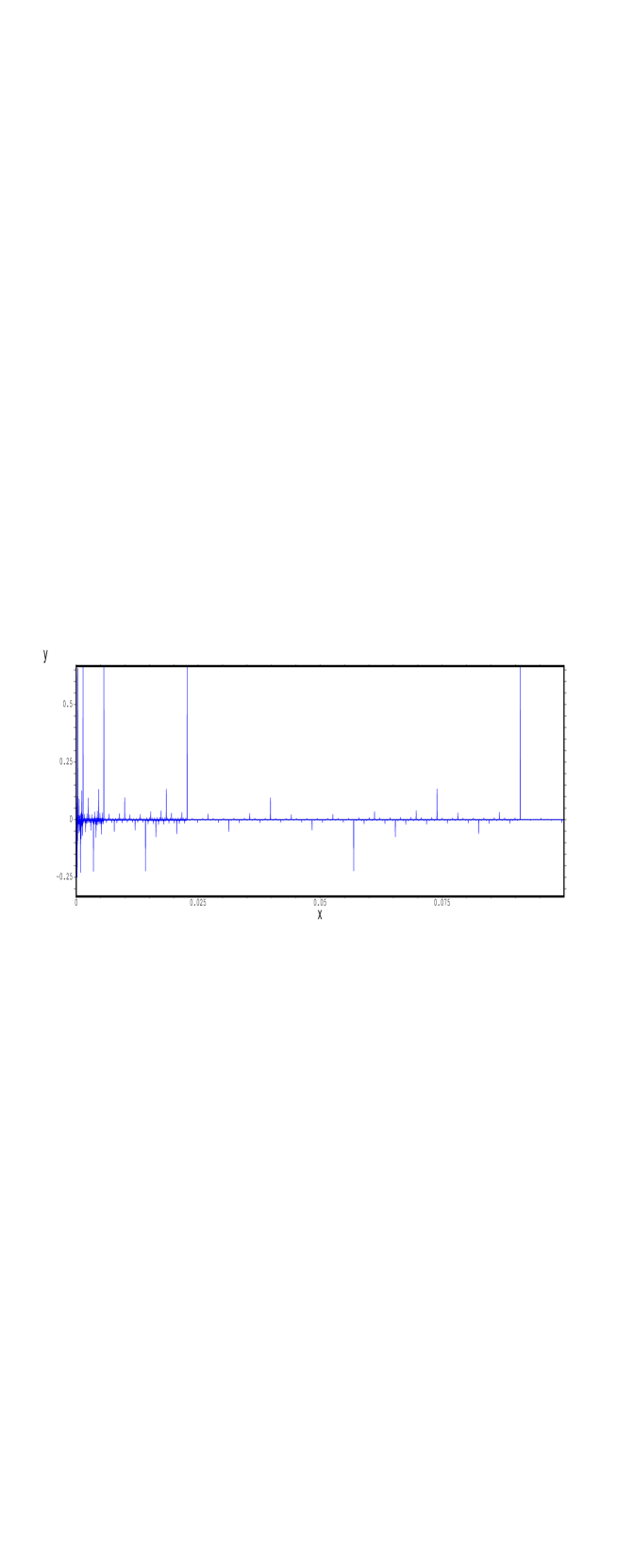
Figure 1. Riesz’s measure: The first 30000 non-zero Verblunsky parameters.

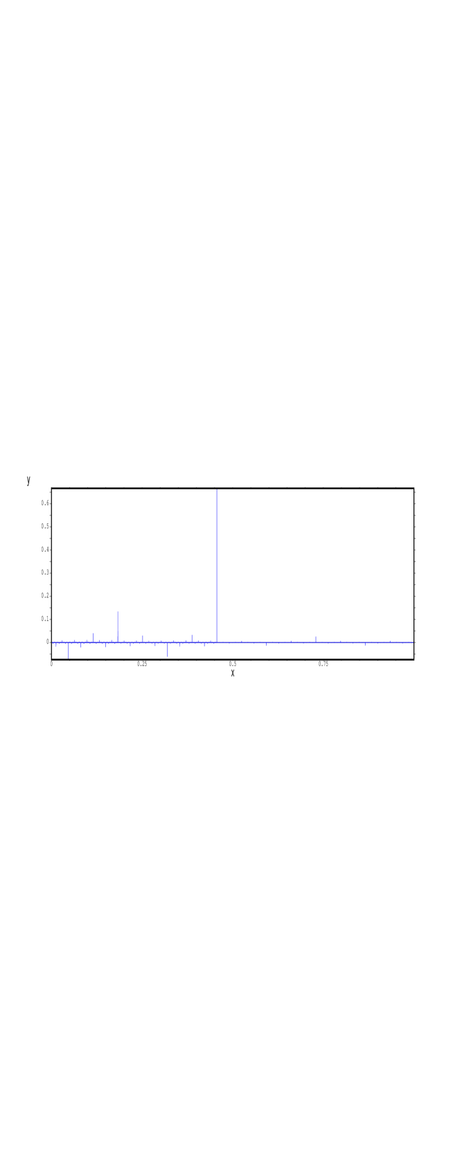
Figure 2. Riesz’s measure: The non-zero Verblunsky parameters for indices between 30000 and 60000.

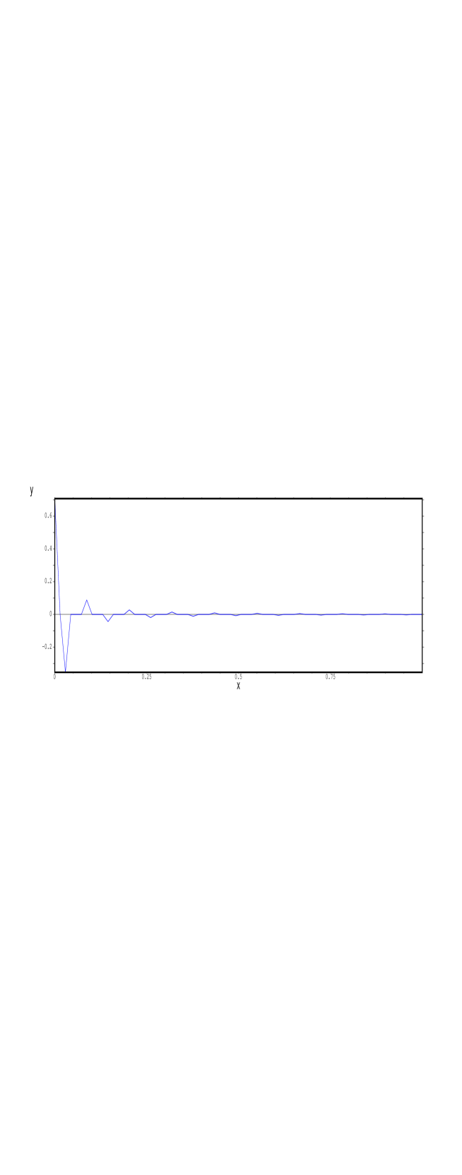
Figure 3. Hadmard’s walk: The first 70 non-zero Taylor coefficients of the Schur function.

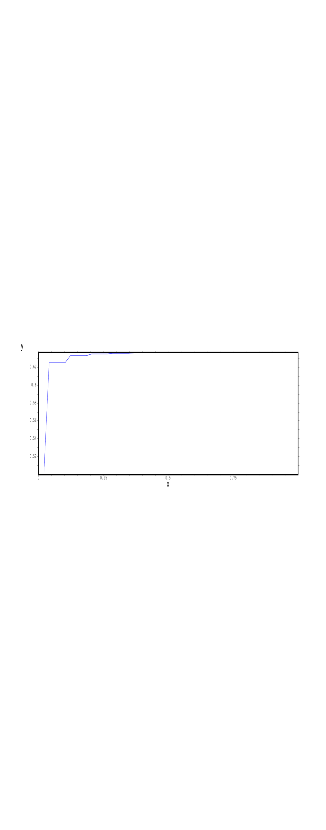
Figure 4. Hadamard’s walk: The cumulative sums of the squares of the first 70 non-zero Taylor coefficients of the Schur function.

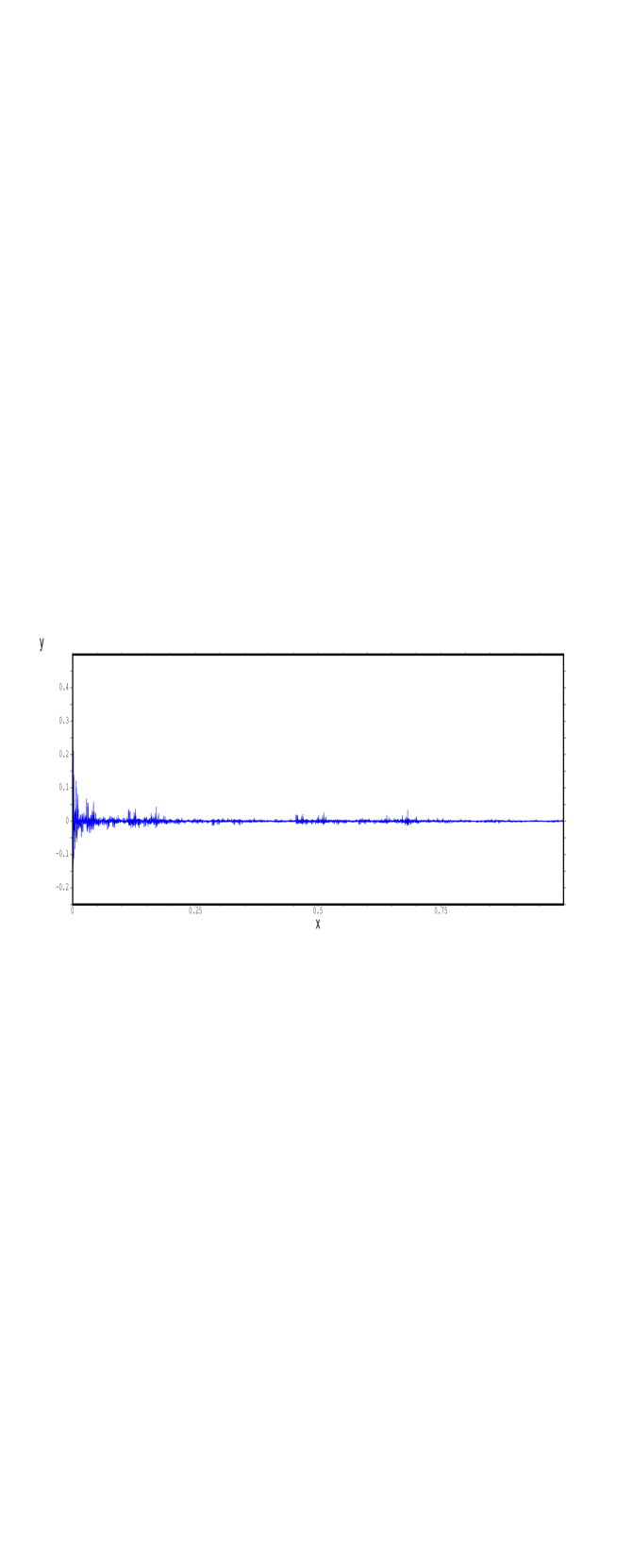
Figure 5. Riesz’s measure: The first 7000 non-zero Taylor coefficients of the Schur function.

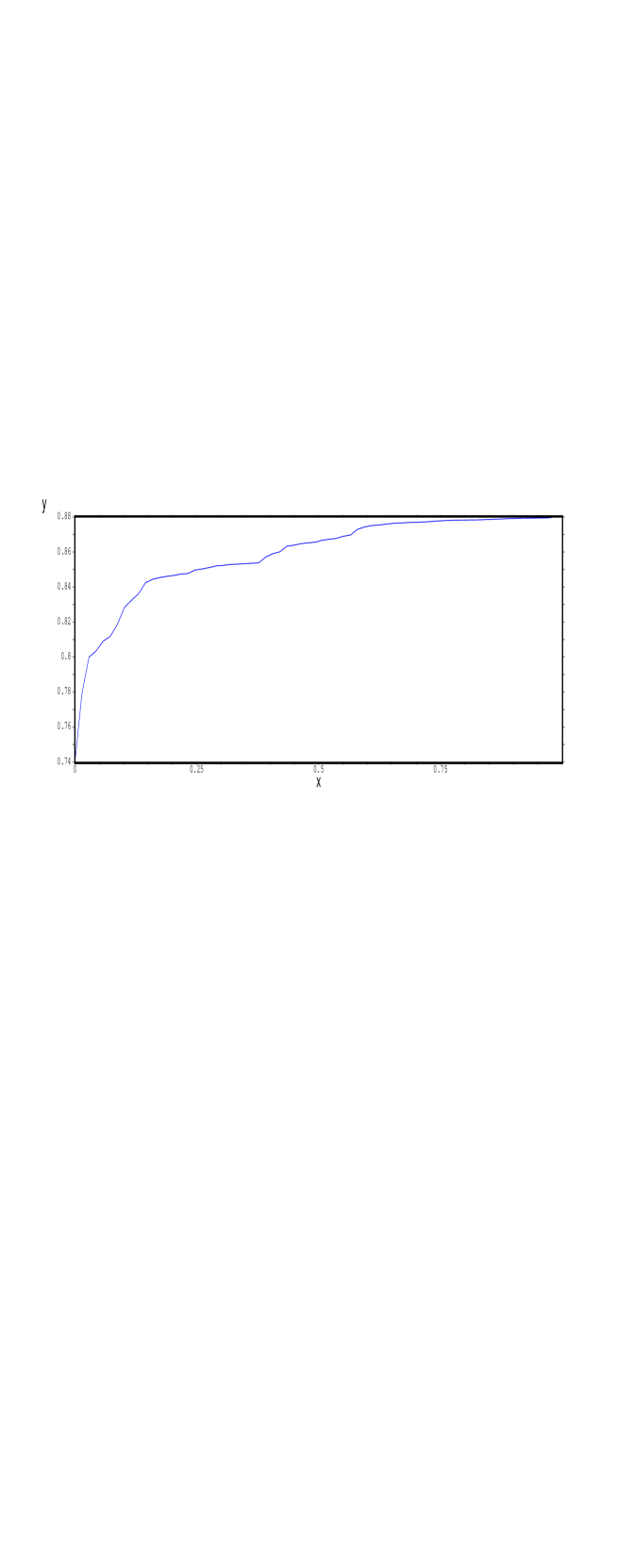
Figure 6. Riesz’s measure: The cumulative sums of the squares of the first 7000 non-zero Taylor coefficients of the Schur function in steps of 100.

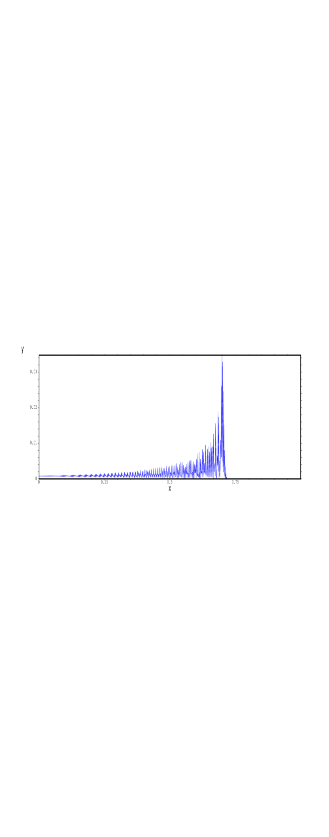
Figure 7. Hadamard’s walk on the non-negative integers: The probability of $X_{n}/n$ for 800 iterations starting at $|0\rangle\otimes|\kern-3.3pt\uparrow\rangle$.

Figure 8. Riesz’s walk on the non-negative integers: The probability of $X_{n}/n$ for 800 iterations starting at $|0\rangle\otimes|\kern-3.3pt\uparrow\rangle$.

References

- [1] A. Ambainis, Quantum walks and their algorithmic applications. International Journal of Quantum Information, 1, (2003) 507–518.
- [2] A. Ambainis, E. Bach, A. Nayak, A. Vishwanath and J. Watrous, One dimensional quantum walks. in Proc. of the ACM Symposium on Theory and Computation (STOC’01), July 2001, ACM, NY, 2001, 37–49.
- [3] O. Bourget, J. S. Howland, and A. Joye, Spectral analysis of unitary band matrices. Commun. Math. Phys., 234, (2003) 191–227.
- [4] M. J. Cantero, L. Moral and L. Velázquez, Five-diagonal matrices and zeros of orthogonal polynomials on the unit circle. Linear Algebra Appl., 362, (2003) 29–56.
- [5] M. J. Cantero, L. Moral and L. Velázquez, Minimal representations of unitary operators and orthogonal polynomials on the unit circle. Linear Algebra Appl., 405, (2005) 40–65.
- [6] M. J. Cantero, F. A. Grünbaum, L. Moral and L. Velázquez, Matrix valued Szegő polynomials and quantum random walks. Commun. Pure Applied Math., 58, (2010) 464–507.
- [7] Ya. L. Geronimus, On polynomials orthogonal on the circle, on trigonometric moment problem, and on allied Carathéodory and Schur functions. Mat. Sb., 15, (1944) 99–130. [Russian]
- [8] C. G. Graham and O. C. McGehee, Essays in Commutative Harmonic Analysis. Springer-Verlag, 1979, Chapter 7.
- [9] F. A. Grünbaum, L. Velazquez, A. Werner and R. Werner, Recurrence for discrete time unitary evolutions. In preparation.
- [10] F. A. Grünbaum and L. Velazquez, The Riesz quantum walk on the integers. In preparation.
- [11] Y. Katznelson, An Introduction to Harmonic Analysis. John Wiley & Sons, 1968.
- [12] J. Kempe, Quantum random walks-an introductory overview. Contemporary Physics, 44, (2003) 307–327.
- [13] N. Konno, Quantum walks. in Quantum Potential Theory, U. Franz, M. Schürmann, editors, Lecture Notes in Mathematics 1954, Springer-Verlag, Berlin, Heidelberg, 2008.
- [14] A. Magnus, Freund equation for Legendre polynomials on a circular arc and solution to the Grünbaum-Delsarte-Janssen-deVries problem. J. Approx. Theory, 139, (2006) 75–90.
- [15] D. Meyer, From quantum cellular automata to quantum lattice gases. J. Stat. Physics, 85, (1996) 551–574, quant-ph/9604003.
- [16] A. Nayak and A. Vishwanath, Quantum walk on the line. Center for Discrete Mathematics Theoretical Computer Science, 2000, quant-ph/0010117.
- [17] G. Pólya, Über eine Aufgabe der Wahrscheinlichkeitsrechnung betreffend die Irrfahrt im Strassennetz. Math. Annalen, 84, (1921) 149–160.
- [18] F. Riesz, Über die Fourierkoeffizienten einer stetigen Funktion von beschränkter Schwankung. Math. Z., 18, (1918) 312–315.
- [19] F. Riesz and B. Sz-Nagy, Functional Analysis. F. Ungar Publishing, New York, 1955.
- [20] W. Rudin, Real and Complex Analysis, second edition. McGraw-Hill Book Co., New York-Düsseldorf-Johannesburg, 1974.
- [21] I. Schur, Über Potenzreihen die im Innern des Einheitskreises beschränkt sind. J. Reine Angew. Math., 147, (1916) 205–232 and 148, (1917) 122–145.
- [22] B. Simon, Orthogonal Polynomials on the Unit Circle, Part 1: Classical Theory. AMS Colloq. Publ., vol. 54.1, AMS, Providence, RI, 2005.
- [23] B. Simon, CMV matrices: Five years after. J. Comput. Appl. Math., 208, (2007) 120–154.
- [24] M. Stefanak, T. Kiss and I. Jex, Recurrence properties of unbiased coined quantum walks on infinite dimensional lattices. arXiv: 0805.1322v2 [quant-ph] 4 Sep 2008.
- [25] G. Szegő, Orthogonal Polynomials, 4th ed. AMS Colloq. Publ., vol. 23, AMS, Providence, RI, 1975.
- [26] H. Wall, Continued fractions and bounded analytic functions. Bull. Amer. Math. Soc., 50, (1944) 110-119.
- [27] D. S. Watkins, Some perspectives on the eigenvalue problem. SIAM Rev., 35, (1993) 430–471.
- [28] A. Zygmund, Trigonometric Series, 2nd ed. Cambridge University Press, 1959.