Estimating cosmic velocity fields from density fields and tidal tensors

Abstract

In this work we investigate the nonlinear and nonlocal relation between cosmological density and peculiar velocity fields. Our goal is to provide an algorithm for the reconstruction of the nonlinear velocity field from the fully nonlinear density. We find that including the gravitational tidal field tensor using second order Lagrangian perturbation theory (2LPT) based upon an estimate of the linear component of the nonlinear density field significantly improves the estimate of the cosmic flow in comparison to linear theory not only in the low density, but also and more dramatically in the high density regions. In particular we test two estimates of the linear component: the lognormal model and the iterative Lagrangian linearisation. The present approach relies on a rigorous higher order Lagrangian perturbation theory analysis which incorporates a nonlocal relation. It does not require additional fitting from simulations being in this sense parameter free, it is independent of statistical-geometrical optimisation and it is straightforward and efficient to compute. The method is demonstrated to yield an unbiased estimator of the velocity field on scales  $>$$\sim$ 5 $h^{-1}\,{\rm Mpc}$ with closely Gaussian distributed errors. Moreover, the statistics of the divergence of the peculiar velocity field is extremely well recovered showing a good agreement with the true one from $N$-body simulations. The typical errors of about 10 km s^-1 (1 sigma confidence intervals) are reduced by more than 80% with respect to linear theory in the scale range between 5 and 10 $h^{-1}\,{\rm Mpc}$ in high density regions ($\delta>2$). We also find that iterative Lagrangian linearisation is significantly superior in the low density regime with respect to the lognormal model.

Works	$\theta$-$\delta$ relation	parameters	methodology
Yahil et al. (1991)	$\theta=\delta$	$\{\mbox{\boldmath$p$}\}$	linear theory: LPT
Nusser et al. (1991)	$\theta=\delta/(1+\alpha\delta)$	$\alpha$, $\{\mbox{\boldmath$p$}\}$	empirical approximation
Bernardeau (1992)	$\theta=\alpha\left[\left(1+\delta\right)^{\beta}-1\right]$	$\alpha,\beta$, $\{\mbox{\boldmath$p$}\}$	PT
Gramann (1993b)	$\theta=\delta-\alpha D_{1}^{2}\mu^{(2)}(\phi_{g})$	$\alpha,\{\mbox{\boldmath$p$}\}$	approx. 2LPT
Willick et al. (1997)	$\theta=\left[(1+\alpha^{2}\sigma^{2}_{\delta})\delta+\alpha\sigma^{2}_{\delta}\right]/(1+\alpha\delta)$	$\alpha,\sigma^{2}_{\delta}$, $\{\mbox{\boldmath$p$}\}$	empirical approximation
Chodorowski et al. (1998)	$\theta=\left[\delta-\alpha\left(\delta^{2}-\sigma^{2}_{\delta}\right)+\beta\delta^{3}\right]$	$\alpha,\beta,\sigma^{2}_{\delta}$, $\{\mbox{\boldmath$p$}\}$	PT+$N$-body
Bernardeau et al. (1999)	$\theta=\left[\gamma\delta+\alpha\left(\delta^{2}-\sigma^{2}_{\delta}\right)+\beta\delta^{3}\right]$	$\alpha,\beta,\gamma,\sigma^{2}_{\delta}$, $\{\mbox{\boldmath$p$}\}$	PT+$N$-body
Kudlicki et al. (2000)	$\theta=\alpha\left[\left(1+\delta\right)^{1/\alpha}-1\right]+(\alpha-1)/(2\alpha)\sigma^{2}_{\delta}$	$\alpha,\sigma^{2}_{\delta}$, $\{\mbox{\boldmath$p$}\}$	PT+Eulerian grid-based code
Bilicki & Chodorowski (2008)	$\theta=\gamma\left[\left(1+\delta\right)^{1/\alpha}-\left(1+\delta\right)^{\beta}\right]$	$\alpha,\beta,\gamma$, $\{\mbox{\boldmath$p$}\}$	spherical collapse model
this work	${\theta}=D_{1}\delta^{(1)}-D_{2}f_{2}/f_{1}\,\mu^{(2)}(\phi^{(1)})$	$\{\mbox{\boldmath$p$}\}$	2LPT

Table 1: The parameters $\alpha,\beta,\gamma$ are either derived from first principles (Bernardeau, 1992; Gramann, 1993b; Bilicki & Chodorowski, 2008, this work) or from fitting to simulations being different for each case. These parameters also depend on the scale of interest. The parameters which are in parenthesis are fully determined by the chosen cosmology and the theoretical model. The variance of the density field is given by $\sigma_{\delta}^{2}=\langle\delta^{2}\rangle$. PT stands for perturbation theory and is applied only in the univariate case (local relation). 2LPT stands for second order Lagrangian perturbation theory and yields the only nonlocal (and nonlinear) relation from the list. Hivon et al. (1995); Monaco & Efstathiou (1999) proposed 2LPT to correct for redshift distortions. Let us mention here the least-action principle methods to determine the peculiar velocities from mass tracer objects (galaxies) introduced by Peebles (1989) and further extended by Nusser & Branchini (2000); Branchini et al. (2002); Lavaux et al. (2008).

1 introduction

Gravitational instability is one of the key ingredients to explain the rich hierarchy of structures we observe today in the Universe. It has amplified small mass fluctuations produced after inflation to give rise from large galaxy clusters to huge voids. Simultaneously, the same local gravitational field imprinted “peculiar” velocities in galaxies; deviations from the overall expansion of the Universe which is responsible for the Hubble flow.

The peculiar velocity of galaxies is a valuable quantity in cosmology since it contains similar but complementary information to that enclosed in the galaxies position. For instance, by requiring isotropy in the measured galaxy clustering, the cosmological mass density parameter and even the nature of gravity can be constrained (see e.g. Davis et al., 1996; Willick & Strauss, 1998; Branchini et al., 2001; Guzzo et al., 2008). In addition, these motions can be used to reconstruct the properties of the universe at an earlier time, in principle, even at recombination where perturbations were completely linear (Nusser & Dekel, 1992; Gramann, 1993a; Croft & Gaztanaga, 1997; Narayanan & Weinberg, 1998; Monaco & Efstathiou, 1999; Frisch et al., 2002).

A method able to accurately determine the peculiar velocity field can be used in many different applications; ranging from bias studies combining galaxy redshift surveys with measured peculiar velocities (see e.g. Fisher et al., 1995; Zaroubi et al., 1999; Courtois et al., 2011), Baryon Acoustic Oscillations reconstructions (see e.g. Eisenstein et al., 2007), determination of the growth factor, to estimates of the initial conditions of the Universe which in turn can be used for constrained simulations (see e.g. Gottloeber et al., 2010; Klypin et al., 2003). A particularly well suited application regards the topological methods to detect the kinematic Sunyaev-Zeldovich effect.

There is in addition recent interest in the measurement of large-scale flows. Some authors claim to have detected a so-called “dark flow” caused by super-horizont perturbations (see e.g. Kashlinsky et al., 2009, 2011). Others discuss such flows as a challenge to the standard cosmological model as a whole (see e.g. Watkins et al., 2009).

Unfortunately, the apparent shift in spectral features of a galaxy is also affected by the expansion of the universe, therefore it is not possible to directly measure the peculiar velocity field in spectroscopic surveys. For this reason, one has to resort to indirectly infer it from the mass density fluctuations (but see Nusser et al., 2011, for a recent alternative method). However, this is not a trivial procedure due the highly nonlinear state of the density fluctuations today and due to its nonlocal relationship with the velocity field.

The simplest approach is given by the linear continuity equation, which is routinely used in clustering studies. However, it has a range of applicability only limited to very large scales (e.g. Angulo et al., 2008). Alternative methods devised to improve upon linear theory can be separated into three areas. The first one consists on developing nonlinear relationships with higher-order perturbation theory (Bernardeau, 1992; Chodorowski et al., 1998; Bernardeau et al., 1999; Kudlicki et al., 2000), with spherical collapse models (Bilicki & Chodorowski, 2008) or based on empirical relations found in cosmological N-body simulations (Nusser et al., 1991; Willick et al., 1997).

Another idea is to solve the boundary problem of finding the initial positions of a set of particles governed by the Eulerian equation of motion and gravity with the least action principle (see Peebles, 1989; Nusser & Branchini, 2000; Branchini et al., 2002). A similar approach consists on relating the observed positions of matter tracers (e.g. galaxies) in a geometrical way to a homogeneous distribution by minimizing a cost function, which combined with the Zeldovich approximation (Zel’dovich, 1970) provides an estimation of the velocity field (see Mohayaee & Tully, 2005; Lavaux et al., 2008).

The diversity of strategies and approximations for obtaining the velocity from the density field hint at the difficulty of the problem. Some approaches are simply not accurate enough and some are computationally very expensive. This sets the agenda for an improvement in the field. Any new method should be accurate, unbiased, computationally efficient and applicable to observational data.

A further shortcoming of the existing approaches is that they are mostly particle-based, which is not applicable for more general matter tracers like the Lyman-alpha forest or the 21-cm line, nor they can be combined with optimal density field estimators (see Kitaura et al., 2010; Jasche & Kitaura, 2009; Kitaura et al., 2010).

In this paper we investigate a different approach based on higher order Lagrangian perturbation theory, and it is motivated by the pioneering work of Gramann (1993b) and further extended by Hivon et al. (1995); Monaco & Efstathiou (1999). The theoretical basis for LPT was carefully worked out by Moutarde et al. (1991); Buchert & Ehlers (1993); Buchert (1994); Bouchet et al. (1995); Catelan (1995) (for further references see Bernardeau et al., 2002).

Contrary to classic applications of LPT, in which the properties of an evolved distribution are predicted from a linear density field in Lagrangian coordinates (e.g. in the generation of initial conditions for $N$-body simulations or of galaxy mock catalogues: Jenkins (2010); Scoccimarro & Sheth (2002)), our starting point is an evolved field in Eulerian coordinates (e.g. the present-day galaxy distribution). The key realisation of our approach is that it is possible to decompose a nonlinear density field into a Gaussian and Non-Gaussian term, which are related to each other through LPT (see similar approaches Gramann, 1993a, b; Monaco & Efstathiou, 1999). In other words, it is possible to find a closely Gaussian field which would evolve, under the assumption of LPT, into the measured density field today. This Gaussian field can then naturally be used to predict the corresponding velocity field today in LPT.

Our method combines i) the equations of motion and continuity for a fluid under self gravity in 2-nd (3-rd) order Lagrangian Perturbation theory (LPT) with ii) the idea that the present-day galaxy distribution can be expanded into a closely linear-Gaussian field and a highly skewed nonlinear component consistent with 2LPT (or 3LPT) (see Kitaura & Angulo, 2011). The former aspect makes our approach physically motivated and also captures the nonlocal nature of the density-velocity relation via the gravitational tidal field tensor. The latter aspect self-consistently minimises the impact of the approximations of a 2nd order formulation of gravitational evolution, but more importantly, it enables the application of LPT to nonlinear fields.

We note that the use of the lognormal transformation (including the subtraction of a mean field) to obtain an estimate of the linear field was proposed by Kitaura et al. (2010) and has been recently confirmed to give already a good estimate of the divergence of the displacement field (Falck et al., 2011). To estimate the velocity field one needs, however, to go to higher order perturbation theory as we show in this work.

In the next section we recap Lagrangian perturbation theory and derive the velocity-density relation to second and third order. In section 2.2 we will present the method to compute the peculiar velocity field from the nonlinear density field. In section 3 we will present our numerical tests based on the Millennium Run simulation. Here we will analyze the goodness of the recovered velocity divergence as compared to the true one and the same for each velocity component. A study of the errors in our method is also presented. Finally we present our conclusions.

2 Velocity–density relation

The first part of this section presents the relation between density and velocity fields in 2LPT, and how it can be applied to an evolved field. In the second part, we outline a practical implementation of this method.

2.1 Second order Lagrangian perturbation theory

The basic idea in Lagrangian perturbation theory is that an initial homogeneous field expressed in Lagrangian coordinates $q$ can be related to a final field in Eulerian coordinates $x$ trough a unique mapping: $\mbox{\boldmath$x$}=\mbox{\boldmath$q$}+\mbox{\boldmath$\Psi$}(\mbox{\boldmath$q$})$ determined by a displacement field $\Psi$ (see e.g. Bernardeau et al., 2002).

The linear solution for this expression is the well-known Zeldovich approximation, in which the displacement field is given by the Laplacian of the gravitational potential at $q$. This result has been successfully applied to many aspects of cosmology, but it fails to describe the dynamics of a nonlinear field where shell crossings and curved trajectories are common.

An improvement is found by expanding the displacement field and considering higher order terms (see e.g. Buchert et al., 1994; Melott et al., 1995; Bouchet et al., 1995). For instance, the displacement field to second order is given by

$$\mbox{\boldmath$\Psi$}(\mbox{\boldmath$q$})=-D_{1}\nabla_{q}\phi^{(1)}(\mbox{\boldmath$q$})+D_{2}\nabla_{q}\phi^{(2)}(\mbox{\boldmath$q$}),$$ (1)

where $D_{1}$ is the linear growth factor normalised to unity today, $D_{2}$ the second order growth factor, which is given by $D_{2}\simeq-3/7\,\Omega^{-1/143}D_{1}^{2}$ (see Buchert & Ehlers, 1993; Bouchet et al., 1995). The potentials $\phi^{(1)}(\mbox{\boldmath$q$})$ and $\phi^{(2)}(\mbox{\boldmath$q$})$ are obtained by solving a pair of Poisson equations: $\nabla^{2}\phi^{(1)}(\mbox{\boldmath$q$})=\delta^{(1)}(\mbox{\boldmath$q$})$, where $\delta^{(1)}$ is the linear over-density, and $\nabla^{2}\phi^{(2)}(\mbox{\boldmath$q$})=\delta^{(2)}(\mbox{\boldmath$q$})$.

It is important to realise that these terms are not independent of each other. The second order nonlinear term $\delta^{(2)}$ is fully determined by the linear over-density field $\delta^{(1)}$ through the following quadratic expression

$$\delta^{(2)}(\mbox{\boldmath$q$})\equiv\mu^{(2)}(\phi^{(1)}(\mbox{\boldmath$q$}))=\sum_{i>j}\Big{(}\phi^{(1)}(\mbox{\boldmath$q$})_{,ii}\phi^{(1)}(\mbox{\boldmath$q$})_{,jj}-[\phi^{(1)}(\mbox{\boldmath$q$})_{,ij}]^{2}\Big{)}\,,$$ (2)

where we use the following notation $\phi_{,ij}(\mbox{\boldmath$q$})\equiv\partial^{2}\phi(\mbox{\boldmath$q$})/\partial q_{i}\partial q_{j}$, and the indices $i,j$ run over the three Cartesian coordinates.

Similarly, the particle co-moving velocities $v$ are given to second order by:

$${\mbox{\boldmath$v$}}(\mbox{\boldmath$q$})=-D_{1}f_{1}H\nabla_{q}\phi^{(1)}(\mbox{\boldmath$q$})+D_{2}f_{2}H\nabla_{q}\phi^{(2)}(\mbox{\boldmath$q$})\,,$$ (3)

where $f_{i}={\rm d}\ln D_{i}/{\rm d}\ln a$, $H$ is the Hubble constant and $a$ is the scale factor. For flat models with a non-zero cosmological constant, the following relations apply $f_{1}\approx\Omega^{5/9},f_{2}\approx 2\Omega^{6/11}$ (see Bouchet et al., 1995), where $\Omega(z)$ is the matter density at a redshift $z$.

We note that going to third order in Lagrangian perturbation theory provides modest improvements (see Buchert & Ehlers, 1993; Melott et al., 1995; Catelan, 1995; Bouchet et al., 1995; Bernardeau et al., 2002).

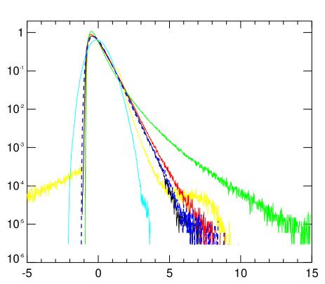
Figure 1: Statistics of the scaled velocity divergence ($\theta_{k}$: true from the simulation $\theta^{\rm Nbody}$ and different reconstructed ones $\theta^{\rm rec}$ as explained below) with different smoothing scales: Left: $r_{\rm S}=$ 5 $h^{-1}\,{\rm Mpc}$, Right: 10 $h^{-1}\,{\rm Mpc}$. Curves from left to right in the order of appearance: yellow: approximate 2LPT solution from the nonlinear density field (GRAM) (see G93 in table 1), cyan: logarithm of the density field (LOG), blue dashed: true scaled velocity divergence at $z=0$ the Millennium Run (Nbody), black: 2LPT estimate from the logarithm of the density field (LOG-2LPT) (Eq. 11), red: 2LPT estimate from the iterative solution (2LPT) (see §2.2), green: linear theory (LIN) (density field).

To apply the Lagrangian framework to a density field in the Eulerian frame $\delta_{\rm M}(\mbox{\boldmath$x$})$ one must be careful. Under the assumption that there is no shell-crossing, one can write the inverse equation relating Eulerian to Lagrangian coordinates $\mbox{\boldmath$q$}=\mbox{\boldmath$x$}-\mbox{\boldmath$\Psi$}(\mbox{\boldmath$x$})$. Mass conservation leads to the following equation (see Nusser et al., 1991):

$$1+\delta_{\rm M}(\mbox{\boldmath$x$})=\tilde{\mbox{\rm\bf J}}(\mbox{\boldmath$x$})\,,$$ (4)

with

$$\tilde{\mbox{\rm\bf J}}(\mbox{\boldmath$x$})\equiv\left|\frac{\partial\mbox{\boldmath$q$}}{\partial\mbox{\boldmath$x$}}\right|\,.$$ (5)

Expanding the Jacobian $\tilde{\mbox{\rm\bf J}}(\mbox{\boldmath$x$})$ one finds (Kitaura & Angulo, 2011);

$$\delta_{\rm M}(\mbox{\boldmath$x$}) = \left|1-\nabla_{x}\cdot\mbox{\boldmath$\Psi$}(\mbox{\boldmath$x$})\right|-1$$ (6)

$$\simeq -\nabla_{x}\cdot\mbox{\boldmath$\Psi$}(\mbox{\boldmath$x$})+\mu^{(2)}(\Theta(\mbox{\boldmath$x$}))+\mu^{(3)}(\Theta(\mbox{\boldmath$x$}))\,.$$

The displacement or velocity field derived from this expression will automatically be expressed in Eulerian coordinates as we will show below. We note that the same expression is found as a function of the Lagrangian coordinate $q$ when expanding the inverse of the corresponding Jacobian $\mbox{\rm\bf J}(\mbox{\boldmath$q$})\equiv\left|{\partial\mbox{\boldmath$x$}}/{\partial\mbox{\boldmath$q$}}\right|$ (see Kitaura & Angulo, 2011).

Using the displacement field (Eq. 1) in Eulerian coordinates, the final density field can be written in terms of the linear and nonlinear fields:

$$\delta_{\rm M}(\mbox{\boldmath$x$})$$ (7)

$$=D_{1}\delta^{(1)}(\mbox{\boldmath$x$})-D_{2}\mu^{(2)}(\phi^{(1)}(\mbox{\boldmath$x$}))+\mu^{(2)}(\Theta(\mbox{\boldmath$x$}))+\mu^{(3)}(\Theta(\mbox{\boldmath$x$}))$$

$$=\delta^{\rm L}(\mbox{\boldmath$x$})+\delta^{\rm NL}(\mbox{\boldmath$x$})\,,$$

with $\Theta(\mbox{\boldmath$x$})$ being the potential associated to the divergence of the displacement field: $\Theta(\mbox{\boldmath$x$})=-\nabla^{-2}\nabla\cdot\mbox{\boldmath$\Psi$}(\mbox{\boldmath$x$})$, $\delta^{\rm L}(\mbox{\boldmath$x$})=D_{1}\delta^{(1)}(\mbox{\boldmath$x$})$ and $\delta^{\rm NL}(\mbox{\boldmath$x$})=-D_{2}\mu^{(2)}(\phi^{(1)}(\mbox{\boldmath$x$}))+\mu^{(2)}(\Theta(\mbox{\boldmath$x$}))+\mu^{(3)}(\Theta(\mbox{\boldmath$x$}))$. The third order term in the Jacobian expansion is given by:

$$\mu^{(3)}(\Theta(\mbox{\boldmath$x$}))=\det\left(\Theta(\mbox{\boldmath$x$})_{,ij}\right)\,.$$ (8)

From now on the Eulerian coordinate dependence $(\mbox{\boldmath$x$})$ is left out.

Assuming that any primordial vorticity has no growing modes associated (the first vorticity terms appear in 3rd order Lagrangian perturbation theory, see appendix) implies that the velocity field today is fully characterised by its divergence ($\nabla\cdot\mbox{\boldmath$v$}$), or, for convenience, by the scaled velocity divergence, defined as:

$$\theta\equiv-{f}(\Omega,\Lambda,z)^{-1}\nabla\cdot\mbox{\boldmath$v$}\,,$$ (9)

with ${f}(\Omega,\Lambda,z)\equiv\dot{D}_{1}/D_{1}=f_{1}(\Omega,\Lambda,z)\,H(z)$.

Combining Eqs. 7 and 3 truncated to quadratic terms in $\Phi^{(1)}$: $\delta^{\rm NL}=\left(D_{1}^{2}-D_{2}\right)\delta^{(2)}$, one gets

$${\theta}=\delta_{\rm M}-\left[D_{1}^{2}+\left(\frac{f_{2}}{f_{1}}-1\right)D_{2}\right]\delta^{(2)}\,.$$ (10)

This expression is very similar to the one found by Gramann (1993b) (see Tab. 1). Note, however, that using directly the evolved field as the source for the second order term $\delta^{(2)}$ is a good approximation for the true velocity field only on very large scales (where $\delta_{\rm M}$ is close to unity), as we will see in §3 and Fig. 1, breaking down on scales of even 10 $h^{-1}\,{\rm Mpc}$ for both estimations of the nonlinear field and of the velocity divergence.

In this paper we follow a different approach, and solve iteratively the following equation;

$${\theta}=D_{1}\delta^{(1)}-D_{2}\frac{f_{2}}{f_{1}}\delta^{(2)}\,.$$ (11)

which results from taking the divergence of Eq. 3. For this, we rely on an estimation of the linear component of the present-day density field, which in turn can be calculated by solving iteratively Eq. (7). Note that the Eulerian description forces one to expand the inverse of the Jacobian (see Eqs. 4-7 and Kitaura & Angulo, 2011). This is the main difference with respect to the work of Monaco & Efstathiou (1999) in which first the Jacobian is expanded and then the inverse of it is taken and could explain why we avoid problems caused by artificial Lagrangian caustics in low density regions as reported in their work.

In practice, a good approximation for the linear term, $\delta^{(1)}$, is simply given by the logarithm of the density field; $\delta^{\rm L}=D_{1}\delta^{(1)}=\ln(1+\delta_{\rm M})-\mu$, with $\mu=\langle\ln(1+\delta_{\rm M})\rangle$, as shown by (Neyrinck et al., 2009; Kitaura & Angulo, 2011). Note that this expression is essentially the lognormal approximation for the matter field (Coles & Jones, 1991). This local transformation has the advantage of being computationally inexpensive.

In summary, approach finds a linear field which when plugged into 2LPT expressions produces the observed matter field (or third order, see appendix). If gravity worked only at a second order level, then this linear field would be identical to the actual linear field that originated $\delta_{\rm M}$, but naturally in reality it is just an approximation. Thus, it is important to characterise the performance and accuracy of the method, which we do in §3. But first, we discuss a practical implementation of our method in the next subsection.

2.2 Method

The method to estimate the peculiar velocity field from the nonlinear density field is straightforward and fast to compute. We now outline the steps to be followed for its implementation. For this, we have assumed that there is an unbiased and complete estimation of the matter field $\delta_{\rm M}$. The extra layer of complication introduced by shot noise, a survey mask, biasing and redshift space distortions is out of the scope of this paper and will be addressed in a future publication.

1. Linear density field

   One starts by computing an estimate of the linear component of the density field. We propose two alternatives for this:

   1. Lognormal model

      $$\delta^{\rm L}_{\rm LOG}=D_{1}\delta^{(1)}=\ln(1+\delta_{\rm M})-\mu$$ (12)

   2. Gaussianisation with LPT (Kitaura & Angulo, 2011)

      $$\delta^{\rm L}_{\rm LPT}=D_{1}\delta^{(1)}=\delta_{\rm M}-\delta^{\rm NL}$$ (13)

2. Linear potential

   Then the Poisson equation is solved to obtain the linear potential:

   $$\phi^{(1)}=\nabla^{-2}\delta^{(1)}$$ (14)

3. Nonlinear second order density field

   The tidal field contribution to second order is calculated from the linear potential:

   $$\delta^{(2)}\left[\phi^{(1)}\right]=\sum_{i>j}\Big{(}\phi^{(1)}_{,ii}\phi^{(1)}_{,jj}-(\phi^{(1)}_{,ij})^{2}\Big{)},$$ (15)

4. Scaled velocity divergence

   One can now construct the 2nd order divergence of the velocity field taking both the linear and the second order contribution:

   $${\theta}=D_{1}\delta^{(1)}-D_{2}\frac{f_{2}}{f_{1}}\delta^{(2)},$$ (16)

5. Peculiar velocity field

   Finally, one obtains the 3D velocity field:

   $$\mbox{\boldmath$v$}=-{f}(\Omega,\Lambda,z)\nabla\nabla^{-2}\theta\,.$$ (17)

Please note that the equations in steps (ib), (ii), (iii) and (v) can be solved with FFTs. Details of the Gaussianisation step with LPT can be found in Kitaura & Angulo (2011).

3 Testing the method with $N$-body simulations

In this section we test the performance of the method outlined above by comparing the velocity field directly extracted from a $N$-body simulation with our estimation based on the respective nonlinear density field.

With this purpose, we employ the Millennium simulation which tracks the nonlinear evolution of more than 10 billion particles in a box of comoving side-length $500$ $h^{-1}\,{\rm Mpc}$ (Springel et al., 2005). In particular, we use the output corresponding to redshift $0$, which is where the most nonlinear structures are present.

At such output we first compute the velocity and density field by mapping the information of dark matter particles onto a grid of $256^{3}$ cells using the nearest-grid-point (NGP) assignment scheme, which gives a spatial resolution of about $2\,$$h^{-1}\,{\rm Mpc}$. We then apply the algorithm presented in §2.2 to infer the velocity divergence on a grid of identical dimensions. In the next two subsections we present our results and explore the accuracy when applied on two scales; 10 $h^{-1}\,{\rm Mpc}$ on which linear theory is usually assumed to perform well, and 5 $h^{-1}\,{\rm Mpc}$ which enters into the mildly nonlinear regime.

3.1 The velocity divergence

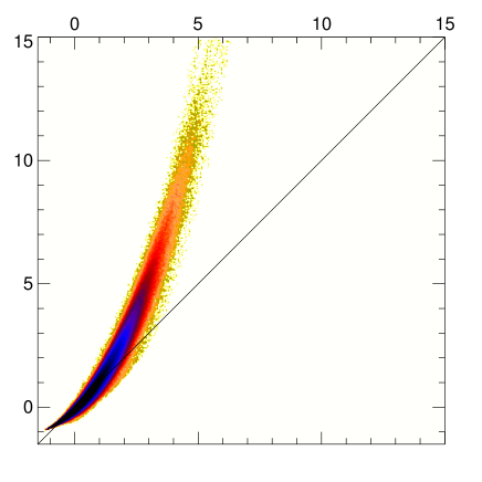
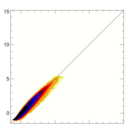
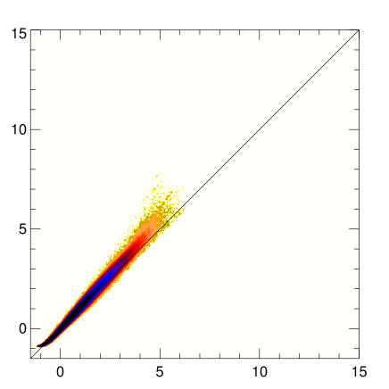
Figure 2: Cell-to-cell comparison between the true and the reconstructed scaled velocity divergence, $\theta^{\rm Nbody}$ and $\theta^{\rm rec}$ respectively. Left panels show results on scales of 5 $h^{-1}\,{\rm Mpc}$ and right panels on scales of 10 $h^{-1}\,{\rm Mpc}$. Upper panels: LIN, middle panels: LOG-2LPT, lower panels: 2LPT. The dark colour-code indicates a high number and the light colour-code a low number of cells.

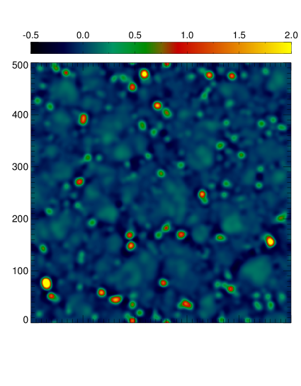
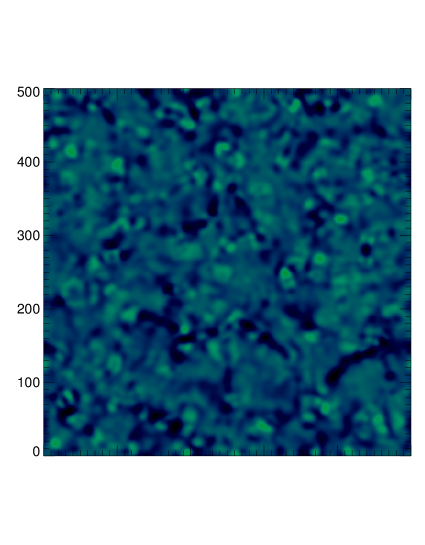
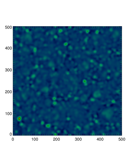
Figure 3: Difference between the true and the estimated scaled velocity divergence. On scales of $r_{\rm S}=$5 $h^{-1}\,{\rm Mpc}$ (left panels) and 10 $h^{-1}\,{\rm Mpc}$ (right panels) with different colour ranges. Upper panels: LIN, middle panels: LOG-2LPT, lower panels: 2LPT.

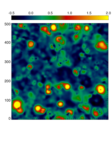
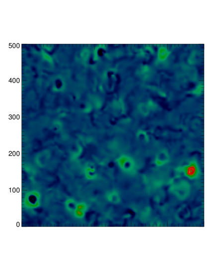
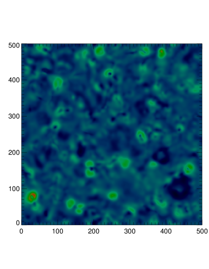
Figure 4: Difference between the true and the estimated speeds (velocity magnitude). On scales of $r_{\rm S}=$5 $h^{-1}\,{\rm Mpc}$ (left panels) and 10 $h^{-1}\,{\rm Mpc}$ (right panels) with different colour ranges. Upper panels: LIN, middle panels: LOG-2LPT, lower panels: 2LPT. The colour-code is in units of $10^{-2}$ s^-1km.

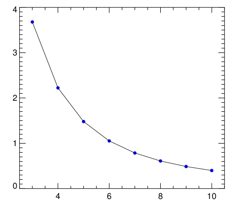
Figure 5: Standard deviation of the $x$-component of the curl $\sigma(\nabla\times\mbox{\boldmath$v$}|_{x})$ divided by the standard deviation of the velocity divergence $\sigma(\nabla\cdot\mbox{\boldmath$v$})$ in % as a function of the scale $r_{\rm S}$. The mean of both the curl and the divergence of the peculiar field are very close to zero.

The first ingredient in our algorithm is the linear component of the density field. We stress that this field are not the “initial conditions” of the universe, since structures have moved from its Lagrangian position to the Eulerian ones at $z=0$. Contrarily to the linear term, the probability distribution function (PDF) of the nonlinear component is highly skewed.

Fig. 1 compares the PDF of the velocity divergence $\theta$ as given by different estimators, with the one directly measured from the simulation (blue dashed line). The left panel shows the fields smoothed with a 5 $h^{-1}\,{\rm Mpc}$ whereas the right panels do so with a larger smoothing of 10 $h^{-1}\,{\rm Mpc}$. In both cases, the predictions of linear perturbation theory (i.e. $\theta=\delta$) displays the worst performance of all – it overestimates systematically the number of volume elements with large value of $\theta$ and underestimates the ones with low values of $\theta$ (green curve). This is a consequence of linear theory breaking down even in mildly under- or overdense regions.

Using linear theory together with the linear component of the nonlinear density field given by the logarithm of the field ($\ln(1+\delta_{\rm M})-\mu$, see cyan curve in Fig. 1) is still a poor description of the PDF, suggesting the need of higher order corrections. We note that this approximation corresponds to linear Lagrangian perturbation theory (Zeldovich approximation).

While standard linear (Eulerian) theory overestimates the values of the divergence of the peculiar velocity field, linear Lagrangian perturbation theory underestimates them. In the former case we are assuming that the scaled divergence of the peculiar velocity field is given by the density field at (final) Eulerian coordinates ($\theta=\delta(\mbox{\boldmath$x$})$), i. e. by the full nonlinear density field; whereas in the latter case we assume that it is given by the density field at (initial) Lagrangian coordinates transformed to Eulerian coordinates ($\theta=D_{1}\delta^{(1)}(\mbox{\boldmath$x$})$), i. e. by the first linear (Gaussian) term in Lagrangian perturbation theory. We note that in general the underestimation of the Zeldovich approximation is less severe (cyan curve) than the overestimation of linear theory (green curve) in high density regions (see Fig. 1). Meaning that the Zeldovich approximation performs better than linear theory being more conservative, as it has been repeatedly shown in the literature (see e.g. Nusser and Branchini 2000). Velocity reconstruction approaches like PIZA or MAK are based on the Zeldovich approximation (see Croft & Gaztanaga, 1997; Lavaux et al., 2008, respectively). We thus expect that the approach presented here is more accurate than these methods.

The first second order estimation we consider is that given by Eq. (10) which is closely related to the one proposed by Gramann and uses the nonlinear field as a proxy for the linear density field (yellow curve). In the regime where this approximation is valid ($\delta\sim 0$) this approach performs remarkably well. However, there is a clear and rapid degradation for volume elements with larger deviations of homogeneity. For instance, this solution yields to values even of $\theta=-140$ at scales of 5 $h^{-1}\,{\rm Mpc}$! This behaviour is due to a complete misestimation of the nonlinear term $\delta^{(2)}$ and therefore of the nonlinear corrections to the velocity field.

Finally, black and red lines indicate the results of the method proposed in this paper: Lagrangian perturbation theory based upon an estimate of the linear component of the density field using the lognormal model (LOG-2LPT: black) or based on the iterative Lagragian linearisation (2LPT: red). In both panels, the predicted PDF very closely follows that measured in the Millennium simulation, even on the extreme tails (especially with LOG-2LPT). The only appreciable difference with the lognormal model is a slight overestimation for low values of $\theta$ (static regions), we note however, that this could be potentially improved by higher order expressions. Indeed, 3rd order PT appears to perform better than 2LPT for underdense regions (see appendix). In spite of this, on both 5 and 10 $h^{-1}\,{\rm Mpc}$ our method is clearly superior to any of the other methods we investigated here, as far as the PDF is concerned and for any value of $\theta$. The iterative 2LPT solution yields a moderate overestimation for high values of $\theta$ due to the laminar flow approximation used in Lagrangian perturbation theory which does not fully capture nonlinear structure formation. Nevertheless, the PDF of $\theta$ using this solution is clearly superior to the linear approximation.

We now continue with a more detailed testing of our method. In Fig. 2 we plot the predicted velocity divergence, $\theta^{\rm rec}_{\rm LOG-2LPT}$ and $\theta^{\rm rec}_{\rm 2LPT}$ (based on $\delta^{\rm L}_{\rm LOG}$ and $\delta^{\rm L}_{\rm LPT}$, respectively), for each of the $256^{3}$ cells in our mesh, as a function of the value measured in the simulation. As in the previous plot, we display results on two different scales; 5 $h^{-1}\,{\rm Mpc}$ on the left panels and 10 $h^{-1}\,{\rm Mpc}$ on the right panels. For comparison we also provide the results using linear perturbation theory $\theta^{\rm rec}_{\rm LIN}=\delta$.

The values of $\theta$ are remarkably well predicted by Lagrangian perturbation theory. In fact, measurements lie around the 1:1 line in the LOG-2LPT case, implying that there are no appreciable biases in our estimation over all the range probed by the Millennium simulation (with the exception of the low values of $\theta$, for an improvement on this see appendix). In contrast, the linear theory prediction presents overestimations of up to a factor of 3 for the 5 $h^{-1}\,{\rm Mpc}$ smoothing and of 2 for 10 $h^{-1}\,{\rm Mpc}$.

The iterative solution (2LPT) produces smaller dispersions but also a slight overestimation of $\theta$ for high values, as we already mentioned before.

The distribution of differences in our method is well approximated by a Gaussian function, whereas in linear theory there are significant extended tails, we will return to this in more detail in §3.2. Overall, this plot suggest that our method not only performs adequately on a statistical basis, but also on predicting the actual average value of $\theta$ in a given volume element.

Although not displayed by the figure, our method also performs better than the other methods shown in Fig. 1. In particular, the classic application of 2LPT recovers $\theta$ quite well for the range $-0.5<\theta<2$, as shown in Gramann (1993b). However, outside this range it displays an erratic behaviour as it could have been anticipated from Fig. 1.

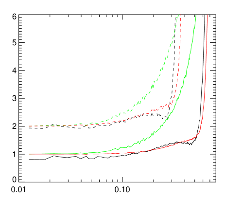
Figure 6: Ratio of the true $P^{\rm Nbody}_{\theta}(k)$ and reconstructed $P^{\rm rec}_{\theta}(k)$ power-spectra of the scaled velocity divergence $\theta$ for green: linear theory (LIN), black: 2LPT estimate from the logarithm of the density field (LOG-2LPT) (Eq. 11), red: 2LPT estimate from the iterative solution (2LPT) (see §2.2). Note that in the case of 10 $h^{-1}\,{\rm Mpc}$ smoothing we have multiplied the lines by a factor of 2 for clarity.

A complementary visual assessment of our method is provided in Fig. 4. In these images we display the relative difference $\theta^{\rm rec}-\theta^{\rm Nbody}$ ($\theta^{\rm rec}_{\rm LIN}-\theta^{\rm Nbody}$ in the upper panels, $\theta^{\rm rec}_{\rm 2LPT}-\theta^{\rm Nbody}$ in the central panels and $\theta^{\rm rec}_{\rm LOG-2LPT}-\theta^{\rm Nbody}$ in the lower ones) projected on a slice 2 $h^{-1}\,{\rm Mpc}$ thick. As previously, we explore 5 and 10 $h^{-1}\,{\rm Mpc}$ and also display the linear theory predictions for comparison. We see that this difference field is not uniformly distributed across the simulation but there are well defined regions in which the prediction is very accurate and others where the prediction is somewhat worse. Not surprisingly the latter coincide with high density regions. Nevertheless, and consistently with previous plots, we see that areas where linear theory fails dramatically are much better handled in our approach.

As a final crucial check, we compute the power-spectra of the scaled velocity divergence according to the $N$-body simulation and our reconstruction with both the LPT and the lognormal linearisation approaches. This is shown in Fig. 6. Linear theory, as expected, increasingly overestimates the power towards small scales, whereas the 2LPT solutions peform remarkably well in a wide range going down to scales of $k\simeq 0.3\,h$/Mpc and $k\simeq 0.5\,h$/Mpc for $r_{\rm S}$=10 $h^{-1}\,{\rm Mpc}$ and $r_{\rm S}$=5 $h^{-1}\,{\rm Mpc}$, respectively. We can also see that there is a systematic deviation originated by the lognormal transformation. The LPT estimate of the linear component corrects these and the results are extremely close to the actual power-spectrum over most of the $k$-range shown.

3.2 The full 3D peculiar velocity field

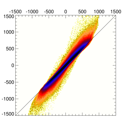
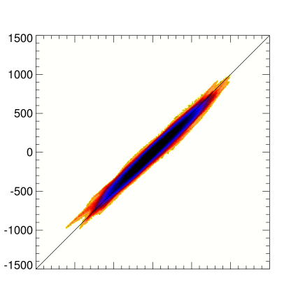
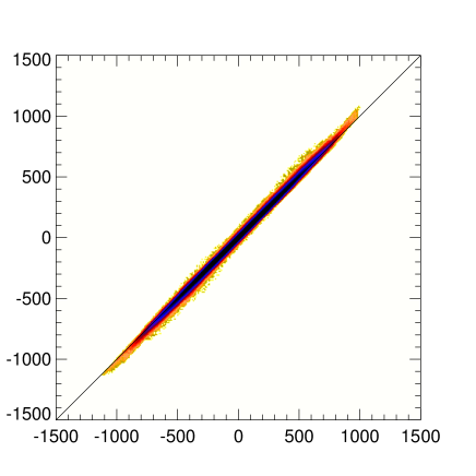
Figure 7: Cell-to-cell comparison between the true velocity $v_{x}^{\rm Nbody}$ and the reconstructed one $v^{\rm rec}_{x}$ for the $x$-component. Left panels on scales of 5 $h^{-1}\,{\rm Mpc}$ and right panels on scales of 10 $h^{-1}\,{\rm Mpc}$. Upper panels: LIN, middle panels: LOG-2LPT, lower panels: 2LPT (see §2.2).

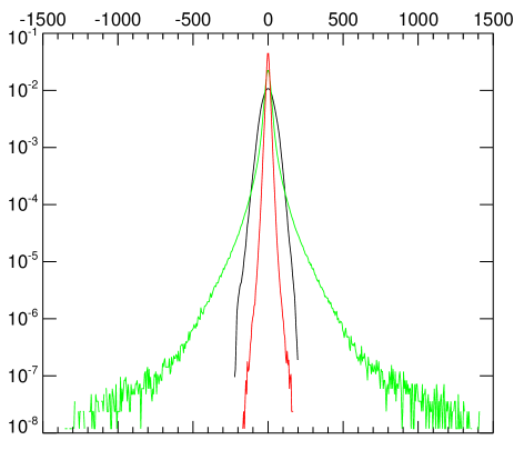
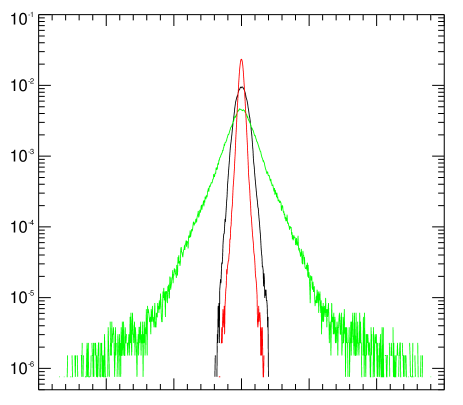
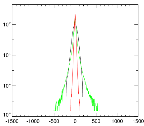
Figure 8: Statistics of the errors in the reconstructed velocity for the $x$-component (green: LIN; black: LOG-LPT, red:2LPT) with different smoothing scales $r_{\rm S}=$ 5 (left panels) and 10 (right panels) $h^{-1}\,{\rm Mpc}$. Upper panels in the entire $\delta$ range, middle panels: for the range $\delta>2$, lower panels: for the range $\delta<0.5$.

We have calculated each component of the peculiar velocity field ($v_{x}$, $v_{y}$,$v_{z}$) from the inferred velocity divergence assuming $\nabla\times\theta=0$. In this case, the Fourier transform of the velocity along a direction is given by $\hat{v}=\mbox{\boldmath$k$}\cdot\hat{\theta}$ with $k$ being the k-vector. The approximation that the velocity field is irrotational is actually a good one for the scales and redshifts we consider here. In fact, the curl of the velocity fields is on average more than 25 times smaller than its divergence in the z=0 output of the Millennium simulation on scales of 3 $h^{-1}\,{\rm Mpc}$ and even smaller on larger scales (see Fig. 5).

In Fig. 7 we compare the velocity field along the x-axis in the simulation and in our method (the two other axis show essentially the same features). The contours show the variation of number of cells (the darker colours represent higher numbers). By comparing both columns, it is clear that linear theory presents biases for large speeds, which are removed by our 2LPT approach, on both 5 and 10 $h^{-1}\,{\rm Mpc}$. We can see that the distribution gets sharper with 2LPT showing a clear decrease in the number of outliers.

We quantified the uncertainty in the recovered velocity in Fig. 8. The x-axis corresponds to the errors in the reconstruction, defined as $\epsilon_{v,x}\equiv v_{x}^{\rm rec}-v_{x}$. As in the previous plot, we show only results for the x-axis since the other three Cartesian coordinates provide consistent results.

We find that the errors in our method are closely Gaussian distributed – the skewness and kurtosis are dramatically smaller than for linear theory. This property is very important when applying the method to real data, since the observational uncertainties can be added to the model uncertainties within a Gaussian likelihood without the need of introducing complex error models. The typical errors are also significantly reduced with smaller standard deviations. The errors in the reconstruction using linear theory have very long tails. Such outliers are not present in our method (see Fig. 8).

As we have discussed along this paper, the larger improvement of our method concerns velocities in high density regions. For regions with $\delta>1$ and $\delta>2$ we find significant differences between linear and 2LPT. At 10 $h^{-1}\,{\rm Mpc}$ and cells with $\delta>2$ the 1 sigma errors with linear theory are about 70 km s^-1 and are reduced with 2LPT to $\sim$13 km s^-1, i.e. 81% smaller. The corresponding 2 sigma confidence intervals are about 160 and 28 km s^-1, respectively, i.e. an error reduction of about 83%. One can see that the 2 sigma confidence intervals are about double as large as the 1 sigma confidence intervals for the 2LPT estimation. However, this is not the case for the linear estimates as these are not Gaussian distributed.

4 Conclusions and discussion

In this paper we presented an improved method to reconstruct the peculiar velocity field from the density field. It builds from 2nd order Lagrangian perturbation theory and the realisation that the density field can be split into a linear plus a nonlinear term. The latter is the key concept, which enables the application of Lagrangian perturbation theory to an evolved field in Eulerian coordinates. This in turn, creates an approach that is nonlinear and nonlocal by including the information of the gravitational tidal field tensor.

We have shown that this approach is efficient and accurate over the dynamical range probed by the Millennium simulation. When the reconstruction is carried out on 5 $h^{-1}\,{\rm Mpc}$, each component of the velocity field can be recovered to an accuracy of about 10 km s^-1. On 10 $h^{-1}\,{\rm Mpc}$ this figure is reduced to about 7 km s^-1. If we consider high density regions, the typical uncertainty is of 13 km s^-1, which improves dramatic over linear perturbation theory; typical errors are 81% smaller. An accurate description of the velocity divergence, both in terms of its PDF and on a point-by-point basis, is also achieved. In addition, we have shown that the 1- and 2-point statistics of the scaled velocity divergence are extremely well recovered, being almost indistinguishable from the true ones. Contrarily, linear theory dramatically over-estimates the velocity divergence. This especially on the mildly nonlinear scale of 5 $h^{-1}\,{\rm Mpc}$ where our method shows more clearly its advantages. Finally, we highlight that our method does not require calibration nor free parameters to predict the velocity divergence field.

There are a number of simplifications and assumptions that we have adopted throughout our paper. First, our analyses focused on the peculiar velocity averaged over a volume. Another aspect is that we have neglected the rotational component of the velocity field. This however, does not seem to be relevant at the scales we have investigated (larger than 5 $h^{-1}\,{\rm Mpc}$). Another simplification is performing our comparison assuming that there is an unbiased estimation of the underlying real-space density field. But, of course, densities measured in a survey are in redshift-space. The transformation can be done, but not trivially. One alternative is to apply the Gibbs-sampling method suggested by Kitaura & Enßlin (2008); Kitaura et al. (2010) to correct for redshift-space distortions. In this, the Gaussian distribution of errors in our method is highly convenient, since it permits to model the uncertainties in the peculiar velocity field including observational errors in a straightforward way. One should consider also classical iterative approaches pioneered by Yahil et al. (1991) based on linear theory. In a similar way they have been applied with different approximations by different groups (see Croft & Gaztanaga, 1997; Nusser & Branchini, 2000; Monaco et al., 2000; Branchini et al., 2002; Mohayaee & Tully, 2005; Lavaux et al., 2008; Wang et al., 2012). Here it is crucial to have an accurate description relating the peculiar velocity field to the density field (or galaxy distribution) which subject of study is central in the work presented here. We expect that the improved relation found in this work with respect to linear Eulerian or linear Lagrangian perturbation theory yields better estimates of the peculiar velocity field. Further studies need to be done to test the performance including redshift-space distortions.

We would like to note that our comparison and the uncertainties quoted here, were based on the present-day output of the Millennium Run. Such simulation was carried out with a value for $\sigma_{8}$ about 10% higher than the current best estimations (see Angulo & White, 2010, for a method to correct for this). Therefore, our uncertainties should be regarded as an upper limit of the reachable uncertainties for a hypothetical spectroscopic survey, which should contain a less nonlinear underlying dark matter distribution.

We finalise this paper by emphasising that the method presented here can potentially be used in many different applications, and should be further developed and tested to perform bias studies combining galaxy redshift surveys with measured peculiar velocities, Baryon Acoustic Oscillation reconstructions, determination of the growth factor, to estimates of the initial conditions of the Universe.

Appendix A Third order Lagrangian perturbation theory (3LPT)

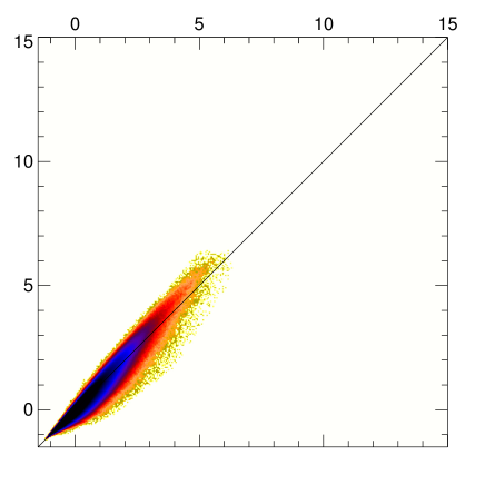
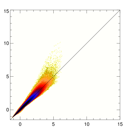
Figure 9: Cell-to-cell correlation between the true and the reconstructed scaled velocity divergence using 3LPT. Left panels on scales of 5 $h^{-1}\,{\rm Mpc}$ and right panels on scales of 10 $h^{-1}\,{\rm Mpc}$. Upper panels: LOG-3LPT (based on the truncated 3LPT expansion computing Eq. 22 with the local model for the linear component), lower panels: 3LPT (based on the truncated 3LPT expansion computing Eq. 24 with the non-local model for the linear component).

For the sake of completeness we investigate here third order LPT. Following Buchert (1994) and Catelan (1995) one can write the displacement field to third order as

$$\Psi = -D_{1}\nabla\phi^{(1)}+D_{2}\nabla\phi^{(2)}$$ (18)

$$+D_{3{\rm a}}\nabla\phi^{(3)}_{{\rm a}}+D_{3{\rm b}}\nabla\phi^{(3)}_{{\rm b}}+D_{3{\rm c}}\nabla\times\mbox{\boldmath$A$}^{(3)}$$

where {$D_{3{\rm a}},D_{3{\rm b}},D_{3{\rm c}}$} are the 3rd order growth factors corresponding to the gradient of two scalar potentials ($\phi^{(3)}_{{\rm a}}$,$\phi^{(3)}_{{\rm b}}$) and the curl of a vector potential ($\mbox{\boldmath$A$}^{(3)}$). Particular expressions for the irrotational 3rd order growth factors ($D_{3{\rm a}},D_{3{\rm b}}$) can be found in Bouchet et al. (1995), the growth factor of the rotational term ($D_{3{\rm c}}$) is given in Catelan (1995).

We assume that the fields are curl-free on scales  $>$$\sim$  5 $h^{-1}\,{\rm Mpc}$ (see Bouchet et al., 1995, and the comparison between the velocity divergence and the curl in the Millennium Run in Fig. 5). We therefore consider only the scalar potential terms $\phi^{(3)}_{{\rm a}}$ and $\phi^{(3)}_{{\rm b}}$.

The first term is cubic in the linear potential

$$\delta^{(3)}_{{\rm a}}\equiv\mu^{(3)}(\phi^{(1)})=\det\left(\phi^{(1)}_{,ij}\right)\,,$$ (19)

and the second term is the interaction term between the first- and the second-order potentials:

$$\delta^{(3)}_{{\rm b}}\equiv\mu^{(2)}(\phi^{(1)},\phi^{(2)})=\frac{1}{2}\sum_{i\neq j}\Big{(}\phi^{(2)}_{,ii}\phi^{(1)}_{,jj}-\phi^{(2)}_{,ij}\phi^{(1)}_{,ji}\Big{)}\,,$$ (20)

(see Buchert, 1994; Bouchet et al., 1995; Catelan, 1995). In order to ensure that the term $\delta^{(3)}_{{\rm b}}$ is curl-free one has to introduce some proper weights in the expression 20 (see Buchert, 1994; Catelan, 1995).

From the displacement field one can derive the expression for the velocity field

$$\mbox{\boldmath$v$}=-D_{1}f_{1}H\nabla\phi^{(1)}+D_{2}f_{2}H\nabla\phi^{(2)}$$

$$+D_{3{\rm a}}f_{3{\rm a}}H\nabla\phi^{(3)}_{{\rm a}}+D_{3{\rm b}}f_{3{\rm b}}H\nabla\phi^{(3)}_{{\rm b}}\,,$$

with $f_{i}={\rm d}\ln D_{i}/{\rm d}\ln a$ (particular expressions for $f_{3{\rm a}}$ and $f_{3{\rm b}}$ can be found in Bouchet et al., 1995). As we can see from Eq. A one can construct all components from the linear potential $\phi^{(1)}$.

We consider here two models for the linear potential. The first model relies on the local lognormal estimate (see §2.2) from which the scaled velocity divergence can be calculated in the following way to 3rd order LPT

$$\theta=D_{1}\delta^{(1)}-\frac{f_{2}}{f_{1}}D_{2}\mu^{(2)}(\phi^{(1)})$$ (22)

$$-\frac{f_{3{\rm a}}}{f_{1}}D_{3{\rm a}}\mu^{(3)}(\phi^{(1)})-\frac{f_{3{\rm b}}}{f_{1}}D_{3{\rm b}}\mu^{(2)}(\phi^{(1)},\phi^{(2)})\,.$$

The second model yields a non-local estimate of $\phi^{(1)}$ to 3rd order given by

$$\delta^{\rm L}=\delta-\delta^{\rm NL}\,$$ (23)

with $\delta^{\rm NL}=-D_{2}\mu^{(2)}(\phi^{(1)})-D_{3{\rm a}}\mu^{(3)}(\phi^{(1)})-D_{3{\rm b}}\mu^{(2)}(\phi^{(1)},\phi^{(2)})+\mu^{(2)}(\Theta)+\mu^{(3)}(\Theta)$. Note that the potential $\Theta$ is also different and is determined by Eq. 18 recalling the relation to the displacement field $\mbox{\boldmath$\Psi$}=-\nabla\Theta$.

Using the latter expression one can write the $\theta$-$\delta$ relation to 3rd order in LPT as

$$\theta=\delta-\left(\frac{f_{2}}{f_{1}}-1\right)D_{2}\mu^{(2)}(\phi^{(1)})$$ (24)

$$-\left(\frac{f_{3{\rm a}}}{f_{1}}-1\right)D_{3{\rm a}}\mu^{(3)}(\phi^{(1)})-\left(\frac{f_{3{\rm b}}}{f_{1}}-1\right)D_{3{\rm b}}\mu^{(2)}(\phi^{(1)},\phi^{(2)})$$

$$-\mu^{(2)}(\Theta)-\mu^{(3)}(\Theta)\,.$$

Note that Eq. 23 should be solved iteratively as we do in the 2LPT case (see §2.2 and Kitaura & Angulo, 2011). Nevertheless to find a fast solution we plug-in the lognormal model for $\phi^{(1)}$ into Eq. 22 yielding a non-local estimate of the linear field in one iteration. To minimize the deviation between LPT and the full nonlinear evolution we have additionally smoothed the density $\delta$ in Eq. 24 with a Gaussian kernel of 2 $h^{-1}\,{\rm Mpc}$ radius.

We do not find an improvement in the determination of the velocity divergence with respect to 2LPT including both curl-free terms using any of the estimates of the linear component. This could be due to an inaccurate determination of the interaction term $\phi^{(3)}_{{\rm b}}$, since uncertainties in the linear component $\phi^{(1)}$ propagate more dramatically than in terms which depend only on the initial conditions ($\phi^{(2)},\phi^{(3)}_{{\rm a}}$).

One may neglect the interaction term $\delta^{(3)}_{{\rm b}}$ and consider only the cubic term $\delta^{(3)}_{{\rm a}}$ to 3rd order. Such a truncated 3LPT model includes the main body of the perturbation sequence with the rest of the sequence being made up of interaction terms (Buchert, 1994).

Our calculations show in this case better results than 2LPT for low values of the velocity divergence (see Fig. 9). However, for large values of $\nabla\cdot\mbox{\boldmath$v$}$ we obtain larger dispersions which could be also due to numerical errors in the estimate of the linear density component $\delta^{\rm L}$. The errors in the velocity estimation are only moderately reduced with respect to the 2LPT case (see §3.2).

References

- Angulo et al. (2008) Angulo R. E., Baugh C. M., Frenk C. S., Lacey C. G., 2008, MNRAS, 383, 755
- Angulo & White (2010) Angulo R. E., White S. D. M., 2010, MNRAS, 405, 143
- Bernardeau (1992) Bernardeau F., 1992, ApJ, 390, L61
- Bernardeau et al. (1999) Bernardeau F., Chodorowski M. J., Łokas E. L., Stompor R., Kudlicki A., 1999, MNRAS, 309, 543
- Bernardeau et al. (2002) Bernardeau F., Colombi S., Gaztañaga E., Scoccimarro R., 2002, Phys.Rep., 367, 1