Correlated singlet phase in the one-dimensional Hubbard-Holstein model

Abstract

We show that a nearest-neighbor singlet phase results (from an effective Hamiltonian) for the one-dimensional Hubbard-Holstein model in the regime of strong electron-electron and electron-phonon interactions and under non-adiabatic conditions ($t/\omega_{0}\leq 1$). By mapping the system of nearest-neighbor singlets at a filling $N_{p}/N$ onto a hard-core-boson (HCB) $t$-$V$ model at a filling $N_{p}/(N-N_{p})$, we demonstrate explicitly that superfluidity and charge-density-wave (CDW) occur mutually exclusively with the diagonal long range order manifesting itself only at one-third filling. Furthermore, we also show that the Bose-Einstein condensate (BEC) occupation number $n_{0}$ for the singlet phase, similar to the $n_{0}$ for a HCB tight binding model, scales as $\sqrt{N}$; however, the coefficient of $\sqrt{N}$ in the $n_{0}$ for the interacting singlet phase is numerically demonstrated to be smaller.

I Introduction

The study of coexistence and competition between diagonal long range orders [such as charge density wave (CDW) and spin density wave (SDW)] and off-diagonal long range orders (such as superfluid and superconducting states) in electronic phases is a subject of immense ongoing focus. Of particular interest is the coexistence of CDW and superconductivity/superfluidity in layered dichalogenides (e.g., 2H-$\rm TaSe_{2}$, 2H-$\rm TaS_{2}$, and $\rm NbSe_{2}$) withers , helium-4 chan , bismuthates (e.g., $\rm BaBiO_{3}$ doped with $\rm K$ or $\rm P$) blanton , quasi-one-dimensional trichalcogenide $\rm NbSe_{3}$ chaikin and doped spin ladder cuprate $\rm Sr_{14}Cu_{24}O_{41}$ abbamonte , quarter-filled organic materials mori ; mckenzie , non-iron based pnictides (e.g., $\rm SrPt_{2}As_{2}$) kudo , etc.

Systems with more than one type of interaction typically manifest a variety of phases of which some cooperate and some compete. A wealth of materials show evidence of strong electron-phonon (e-ph) interactions besides the ubiquitous electron-electron (e-e) interactions. For instance, transition metal oxides such as cuprates photoem1 ; photoem3 and manganites lanzara2 ; pbl ; boothroyd and molecular solids such as fullerides fullarene3 indicate strong e-ph coupling. The interplay of e-e and e-ph interactions in these correlated systems leads to coexistence of or competition between various phases such as superconductivity, CDW, SDW, etc.

An archetypal model for understanding the co-occurring effects of e-e and e-ph interactions is the following well known Hubbard-Holstein model (HHM) sryspbl1

$$H_{hh}\! = \!-t\sum_{j\sigma}\left(c^{\dagger}_{j+1\sigma}c_{j\sigma}+{\rm H.c.}\right)+\omega_{0}\sum_{j}a_{j}^{\dagger}a_{j}$$ (1)

$$+g\omega_{0}\sum_{j\sigma}n_{j\sigma}(a_{j}+a_{j}^{\dagger})+U\sum_{j}n_{j\uparrow}n_{j\downarrow},$$

where $c_{j\sigma}^{\dagger}$ is the fermionic creation operator for itinerant spin-$\sigma$ electrons with hopping integral $t$ and number operator $n_{j\sigma}\equiv c_{j\sigma}^{\dagger}c_{j\sigma}$, $a_{j}^{\dagger}$ is the corresponding bosonic creation operator characterized by a dispersionless phonon frequency $\omega_{0}$, with $U$ and $g$ representing the strengths of onsite e-e and e-ph interactions respectively.

To understand the interplay between the e-e and e-ph interactions, the Hubbard-Holstein model has been extensively studied (in one-, two-, and infinite-dimensions and at various fillings) by employing various approaches such as exact diagonalization exdiag1 ; exdiag2 ; exdiag4 , density matrix renormalization group (DMRG)dmrg ; dmrg2 , quantum Monte Carlo (QMC) qmc1 ; qmc3 ; qmc4 ; qmc5 ; qmc6 ; qmc7 , semi-analytical slave boson approximations slave_b1 ; slave_b2 ; slave_b3 ; slave_b4 ; slave_b5 , dynamical mean field theory (DMFT) dmft1 ; dmft2 ; dmft3 ; dmft4 ; dmft5 ; dmft6 ; dmft7 ; dmft8 ; dmft9 , large-N expansion largeN2 , variational methods based on Lang-Firsov transformation lf1 ; lf2 , Gutzwiller approximation GA1 ; GA2 , and cluster approximation vca .

In our earlier worksryspbl1 , in the regimes of strong Coulomb interaction and strong e-ph coupling, we derived an effective Hamiltonian using a controlled analytic approach that takes into account dynamical quantum phonons. We solved this effective Hamiltonian numerically for finite chains and presented a phase diagram for the one-dimensional Hubbard-Holstein model at quarter filling. It was shown in Ref. sryspbl1, that while the e-e interaction produces nearest-neighbor (NN) spin antiferromagnetic (AF) interactions which encourage singlet formation, the e-ph interaction generates NN repulsion which is expected to promote CDW order. It was also shown that a correlated NN singlet phase occurs (at quarter-filling) and that it carries a signature of a CDW. In this paper, we demonstrate that the correlated singlet phase occurs at other fractions as well and analyze its nature. Our main result is the demonstration that the NN spin AF and NN repulsive interactions compete (instead of cooperate) to produce mutually exclusive (rather than coexisting) superfluid and CDW phases in the NN singlet phase. We show that the NN singlets manifest superfluidity (and no CDW) at all fillings that are less than one-half but not equal to one-third and a CDW state (and no superfluidity) at one-third filling. Using a modified Lanczos method sryspbl1 ; dagotto and a newly developed world-line quantum Monte Carlo (WQMC) method we show that the singlet phase has no Bose-Einstein condensate (BEC) fraction.

In the past, superconductivity due to onsite pairing has been a focus of a number of studies alex ; ranninger ; hardikar . Here we are interested in a different situation, namely, NN singlets. Earlier a $t$-$J$-$V$ model (involving bipolarons that are NN singlets) was introduced in Ref. bonca, . This $t$-$J$-$V$ model bonca [that does not include the next-nearest-neighbor hopping terms but discusses them qualitatively] is similar to our effective Hamiltonian of Eq. (9) and can be regarded as a useful precedent and an endorsement of Eq. (9).

The paper is organised as follows: in Sec. II we briefly derive the effective Hamiltonian (that goes beyond the $t-J$ model approximation of the Hubbard model by including the additional three site residue eder ; troyer ; bala ) and explain the various interaction terms and hopping terms. We also point out that the correlated singlet phase occurs at not only quarter-filling but also at other fillings. In Sec. III, we show that the correlated singlet phase can be represented by a hard-core-boson (HCB) $t\!\!-\!\!V_{1}\!\!-\!\!V_{2}$ model. Next, in Sec. IV we discuss the possibility of formation of a CDW by mapping the $t\!\!-\!\!V_{1}\!\!-\!\!V_{2}$ model onto the well understood $t$-$V$ model. In Sec V, we obtain the superfluid density (in the thermodynamic limit) at different filling fractions by using finite size scaling. In Sec. VI, we analyze the BEC occupation number at various densities by employing the modified Lanczos method and a newly developed WQMC method. We close with concluding remarks in Sec. VII.

II Effective HHM Hamiltonian

We briefly outline below the procedure to get the effective Hubbard-Holstein Hamiltonian (with more details being provided in Ref. sryspbl1, ). Although we obtain the effective Hamiltonian here in one-dimension only, our approach is easily extendable to higher dimensions as well. We first carry out the Lang-Firsov (LF) transformation LF_transf $H^{LF}_{hh}=e^{T}H_{hh}e^{-T}$ where $T=-g\sum_{j\sigma}n_{j\sigma}(a_{j}-a_{j}^{\dagger})$ and get the following LF transformed Hamiltonian:

$$H^{LF}_{hh} = -t\sum_{j\sigma}(X_{j+1}^{\dagger}c_{j+1\sigma}^{\dagger}c_{j\sigma}X_{j}+{\rm H.c.})+\omega_{0}\sum_{j}a_{j}^{\dagger}a_{j}$$ (2)

$$-g^{2}\omega_{0}\sum_{j}n_{j}+(U-2g^{2}\omega_{0})\sum_{j}n_{j\uparrow}n_{j\downarrow},$$

where $X_{j}=e^{g(a_{j}-a_{j}^{\dagger})}$ and $n_{j}=n_{j\uparrow}+n_{j\downarrow}$. Next, we express as follows our LF transformed Hamiltonian in terms of the composite fermionic operator $d_{j\sigma}^{\dagger}\equiv c_{j\sigma}^{\dagger}X_{j}^{\dagger}$:

$$H^{LF}_{hh}=-t\sum_{j\sigma}\left(d_{j+1\sigma}^{\dagger}d_{j\sigma}+{\rm H.c.}\right)+\omega_{0}\sum_{j}a_{j}^{\dagger}a_{j}$$

$$+(U-2g^{2}\omega_{0})\sum_{j}n_{j\uparrow}^{d}n_{j\downarrow}^{d}-g^{2}\omega_{0}\sum_{j}\left(n_{j\uparrow}^{d}+n_{j\downarrow}^{d}\right),$$ (3)

where $n_{j\sigma}^{d}=d_{j\sigma}^{\dagger}d_{j\sigma}$. On dropping the last term, which is a constant polaronic energy, we recognize that Eq. (3) essentially represents the Hubbard Model for composite fermions with Hubbard interaction $U_{eff}=(U-2g^{2}\omega_{0})$. In the limit of large $U_{eff}/t$, using standard treatment involving a canonical transformation, we get the following effective Hamiltonian written to second order in the small parameter $t/U_{eff}$eder ; troyer ; bala :

$$H_{t-J-t_{3}} = P_{s}\left[-t\sum_{j\sigma}\left(d_{j+1\sigma}^{\dagger}d_{j\sigma}+{\rm H.c.}\right)+\omega_{0}\sum_{j}a_{j}^{\dagger}a_{j}\right.$$ (4)

$$+ J\sum_{j}\left(\vec{S}_{j}\cdot\vec{S}_{j+1}-{n_{j}^{d}n_{j+1}^{d}\over{4}}\right)$$

$$+ t_{3}\sum\limits_{j\sigma}\left[d_{j\bar{\sigma}}^{\dagger}d_{j+1\sigma}d_{j-1\sigma}^{\dagger}d_{j\bar{\sigma}}+{\rm H.c.}\right]$$

$$- \left.t_{3}\sum\limits_{j\sigma}\left[d_{j\sigma}^{\dagger}d_{j+1\sigma}d_{j-1\bar{\sigma}}^{\dagger}d_{j\bar{\sigma}}+{\rm H.c.}\right]\right]P_{s},$$

where $n_{j}^{d}=n_{j\uparrow}^{d}+n_{j\downarrow}^{d}$, $J={4t^{2}\over{U-2g^{2}\omega_{0}}}$, $t_{3}=J/4$, $\vec{S}_{i}$ is the spin operator for a spin $1/2$ fermion at site $i$, and $P_{s}$ is the single-occupancy-subspace projection operator. Furthermore, the last two terms with coefficient $t_{3}$ ($=J/4$) are the three site terms which when omitted from the above Hamiltonian $H_{t-J-t_{3}}$ yield the well-known $t-J$ Hamiltonian (for the composite fermionic operators $d_{j\sigma}$).

The effective $t-J-t_{3}$ Hamiltonian, given in Eq. (4), can be re-written in terms of the original fermionic operators $c_{j\sigma}$ as

$$H_{t-J-t_{3}}=H_{0}+H_{1},$$ (5)

where

$$H_{0} = -te^{-g^{2}}\sum_{j\sigma}P_{s}\left(c_{j+1\sigma}^{\dagger}c_{j\sigma}+{\rm H.c.}\right)P_{s}+\omega_{0}\sum_{j}a_{j}^{\dagger}a_{j}$$ (6)

$$+J\sum_{j}P_{s}\left(\vec{S}_{j}\cdot\vec{S}_{j+1}-{n_{j}n_{j+1}\over{4}}\right)P_{s}$$

$$+\frac{Je^{-g^{2}}}{4}\sum\limits_{j\sigma}P_{s}\left[c_{j\bar{\sigma}}^{\dagger}c_{j+1\sigma}c_{j-1\sigma}^{\dagger}c_{j\bar{\sigma}}+{\rm H.c.}\right]P_{s}$$

$$- \frac{Je^{-g^{2}}}{4}\sum\limits_{j\sigma}P_{s}\left[c_{j\sigma}^{\dagger}c_{j+1\sigma}c_{j-1\bar{\sigma}}^{\dagger}c_{j\bar{\sigma}}+{\rm H.c.}\right]P_{s},$$

and

$$\!\!\!\!\!H_{1} = -te^{-g^{2}}\!\sum_{j\sigma}P_{s}\!\left[c_{j+1\sigma}^{\dagger}c_{j\sigma}(Y_{+}^{j\dagger}Y_{-}^{j}-1)+{\rm H.c.}\right]\!P_{s}.$$ (7)

In the above equation, we have separated the $H_{t-J-t_{3}}$ Hamiltonian into (i) an electronic part $H_{0}$ which is essentially a modified $t-J-t_{3}$ Hamiltonian containing a NN hopping with a reduced amplitude ($te^{-g^{2}}$), electronic interaction terms with the same interaction strength $J$, three site terms with reduced amplitude $Je^{-g^{2}}/4$, and no electron-phonon interaction; and (ii) the remaining perturbative part $H_{1}$ which corresponds to the composite fermion terms containing the e-ph interaction with $Y^{j}_{\pm}\equiv e^{\pm g(a_{j+1}-a_{j})}$. Furthermore, since $J/4<<t$, we have ignored the following term in $H_{1}$

$$\!\!\!\!P_{s}\left[\frac{Je^{-g^{2}}}{4}\sum\limits_{j\sigma}\left[c_{j\bar{\sigma}}^{\dagger}c_{j+1\sigma}c_{j-1\sigma}^{\dagger}c_{j\bar{\sigma}}(Z_{+}^{j\dagger}Z_{-}^{j}-1)+{\rm H.c.}\right]\right.$$

$$-\left.\frac{Je^{-g^{2}}}{4}\sum\limits_{j\sigma}\left[c_{j\sigma}^{\dagger}c_{j+1\sigma}c_{j-1\bar{\sigma}}^{\dagger}c_{j\bar{\sigma}}(Z_{+}^{j\dagger}Z_{-}^{j}-1)+{\rm H.c.}\right]\right]P_{s},$$

(8)

where $Z^{j}_{\pm}\equiv e^{\pm g(a_{j-1}-a_{j+1})}$.

After carrying out perturbation theory to second-order (as outlined in Ref. sryspbl1, and Appendix A), with $t/(g\omega_{0})$ as the small parameter ravindra , we get the following effective Hamiltonian:

$$H_{hh}^{eff} \cong -t_{eff}h_{t_{1}}+Jh_{S}-Vh_{nn}-t_{2}h_{\sigma\sigma}$$ (9)

$$-(t_{2}+J_{3})h_{\sigma\bar{\sigma}}+J_{3}h_{\sigma\bar{\sigma}}^{\prime}$$

where

$$h_{t_{1}}=\sum\limits_{j\sigma}P_{s}\left(c_{j+1\sigma}^{\dagger}c_{j\sigma}+{\rm H.c.}\right)P_{s},$$ (10)

$$h_{S}=\sum\limits_{j}P_{s}\left(\vec{S}_{j}\cdot\vec{S}_{j+1}-\frac{1}{4}n_{j}n_{j+1}\right)P_{s},$$ (11)

$$h_{nn}=\sum\limits_{j\sigma}(1-\!\!n_{j+1\bar{\sigma}})(1-\!n_{j\bar{\sigma}})(n_{j\sigma}-n_{j+1\sigma})^{2},$$ (12)

$$h_{\sigma\sigma} =\sum\limits_{j\sigma}(1-n_{j+1\bar{\sigma}})(1-n_{j\bar{\sigma}})(1-n_{j-1\bar{\sigma}})$$ (13)

$$~{}~{}~{}~{}~{}~{}\times\left[c_{j+1\sigma}^{\dagger}(1-2n_{j\sigma})c_{j-1\sigma}+{\rm H.c.}\right],$$

$$h_{\sigma\bar{\sigma}} =\sum\limits_{j\sigma}(1-n_{j+1\bar{\sigma}})(1-n_{j-1\sigma})$$ (14)

$$~{}~{}~{}~{}~{}~{}\times\left[c_{j\sigma}^{\dagger}c_{j+1\sigma}c_{j-1\bar{\sigma}}^{\dagger}c_{j\bar{\sigma}}+{\rm H.c.}\right],$$

and

$$h_{\sigma\bar{\sigma}}^{\prime} =\sum\limits_{j\sigma}(1-n_{j+1\bar{\sigma}})(1-n_{j\sigma})(1-n_{j-1\bar{\sigma}})$$ (15)

$$~{}~{}~{}~{}~{}~{}\times\left[c_{j\bar{\sigma}}^{\dagger}c_{j+1\sigma}c_{j-1\sigma}^{\dagger}c_{j\bar{\sigma}}+{\rm H.c.}\right].$$

The various coefficients are defined in terms of the system electron-phonon coupling $g$, the Hubbard interaction $U$, the hopping amplitude $t$, and the phonon frequency $\omega_{0}$ as follows: $V\simeq t^{2}/{2g^{2}\omega_{0}}$, $J\equiv{4t^{2}\over{U-2g^{2}\omega_{0}}}$, $t_{eff}\equiv te^{-g^{2}}$, $t_{2}\simeq t^{2}e^{-g^{2}}/{g^{2}\omega_{0}}$, and $J_{3}=Je^{-g^{2}}/4$. Here the kinetic energy (which is small compared to the interaction energy) has contributions from four hopping terms: $-t_{eff}h_{t_{1}}$ corresponding to NN hopping (with a reduced hopping integral $t_{eff}{\equiv te^{-g^{2}}}$), $-t_{2}h_{\sigma\sigma}$ representing NNN hopping (with double-hopping coefficient $t_{2}{\simeq t^{2}e^{-g^{2}}/{g^{2}\omega_{0}}}$), $-(t_{2}+J_{3})h_{\sigma\bar{\sigma}}$ implying NN spin-pair $\sigma\bar{\sigma}$ hopping, and $J_{3}h_{\sigma\bar{\sigma}}^{\prime}$ leading to NN spin-pair $\sigma\bar{\sigma}$ hopping and flipping to $\bar{\sigma}\sigma$; thus $h_{\sigma\bar{\sigma}}^{\prime}$ acting on a singlet state produces another singlet state, but with a negative sign. The NN spin-spin interaction term $Jh_{S}$ (with $J\equiv{4t^{2}\over{U-2g^{2}\omega_{0}}}$) and the NN repulsion term $-Vh_{nn}$ (with $V\simeq t^{2}/{2g^{2}\omega_{0}}$) are the dominant terms in the effective Hamiltonian and compete to form a phase separated cluster at larger $J$ (or smaller $U/t$ at a fixed $g$ and $t/\omega_{0}$). As $J/V$ decreases, the cluster breaks up to undergo a discontinuous transition to a correlated NN singlet phase as shown in the phase diagram [see Fig. 1(a)]adiab0.5 . At even lower values of $J/V$, we get separated single spins (represented by isolated spin phase) with the transition at larger $g$ being first-order while at smaller $g$ it is weakly first order and not continuous [due to the fact that the system transforms from a superfluid to a CDW, i.e., transition is between two phases of different symmetry]sryspbl1 . The prime objective of the current work is to characterize the correlated singlet state.

We will now compare the physics related to our effective Hamiltonian, which accounts for various fundamental processes involved in the kinetic and interaction terms, with the variational Lang-Firsov (LF) treatments reported slave_b4 ; slave_b5 ; dmft7 ; lf2 ; GA2 . As the degree of non-adiabaticity decreases, our NNN hopping term $-t_{2}h_{\sigma\sigma}$ contribution increases, effectively the hopping transport will be larger than that given by $-t_{eff}h_{t_{1}}$; these two hopping terms together can be regarded as producing a less than $e^{-g^{2}}$ suppression of the hopping integral reported in earlier variational LF treatments. Furthermore, concerning the effect of including a large Hubbard $U$ term in a Holstein model, we get the NN interaction $2V$ reduced to $2V-J/4$; thus, the mobility would be enhanced which is consistent again with the earlier works using variational LF transformation.

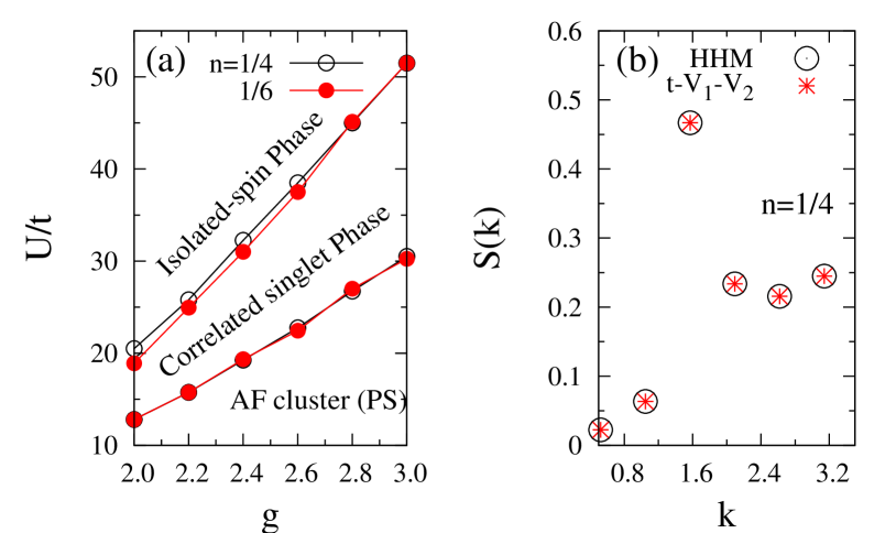
Figure 1: (Color online) Plots obtained using modified Lanczos in a twelve-site system for $t/\omega_{0}=1$. Phase diagram in (a) depicts that the phase transition lines are close for both densities $n=1/4$ and $n=1/6$. Structure factor plots in (b) (drawn at $g=2.2$ and $U/t=17$) for the effective Hubbard-Holstein model (HHM) of Eq. (9) and the HCB $t$-$V_{1}$-$V_{2}$ model of Eq. (16) showing that the two models are equivalent.

III $t$-$V_{1}$-$V_{2}$ hard-core-boson (HCB) model

In the rest of the paper we study the correlated singlet phase. No pair of singlets can share a common site. The closest two singlets can approach each other is to have one spin from each singlet be on adjacent sites. The singlets transport via two processes: (i) the NN spin-pair $\sigma\bar{\sigma}$ hopping given by the $h_{\sigma\bar{\sigma}}$ and $h_{\sigma\bar{\sigma}}^{\prime}$ terms in Eq. (9); and (ii) a second order process involving breaking of a bound singlet state [with binding energy $E_{B}=-J+t^{2}/(g^{2}\omega_{0})$] and hopping of the two constituent spins (of the singlet) to (a) neighboring sites in the same direction sequentially [yielding the term $-t_{b}h_{\sigma\bar{\sigma}}$ with $t_{b}\equiv t^{2}e^{-2g^{2}}/|E_{B}|$] or (b) neighboring sites in opposite direction and back [yielding the term $-t_{b}h_{nn}$]. We now make the important observation that a NN singlet can be represented as a HCB located at the center of the singlet. Thus the system of NN singlets in a periodic lattice is transformed into a system of HCB also in a periodic lattice with the same lattice constant $a$ but with the whole lattice displaced by $a/2$. Then the effective Hamiltonian of the HCB system is the following $t$-$V_{1}$-$V_{2}$ model:

$$\!\!\!\!\!\!\!\!\!\!\!\!\!H_{b}=\!\sum\limits_{j}[-T(b^{\dagger}_{j}b_{j+1}+{\rm H.c.})+V_{1}n_{j}n_{j+1}+V_{2}n_{j}n_{j+2}],$$ (16)

where $b_{j}$ is the HCB destruction operator, $n_{j}=b^{\dagger}_{j}b_{j}$, $T\equiv(t_{2}+2J_{3}+t_{b})$, $V_{1}=\infty$ (because two singlets cannot share a site), and $V_{2}\simeq 2V-J/4$ [with $V_{2}/T>10$ (i.e., $V_{2}/T>>1$) for parameter values in the singlet regime of our phase diagrams in Fig. 1(a)]. In the following we set $T=1$. We corroborate our mapping of the effective HHM Hamiltonian $H_{hh}^{eff}$ (for the singlet phase) onto the HCB Hamiltonian $H_{b}$ by demonstrating in Fig. 1(b) that the static structure factor $S(k)\equiv\sum_{l}e^{ikl}W(l)$ for the HHM and HCB cases coincide when the correlation function $W(l)\equiv(1/N)\sum_{j}[\langle A_{j}A_{j+l}\rangle-\langle A_{j}\rangle\langle A_{j+l}\rangle]$ is defined through $A_{j}\equiv(S^{+}_{j}S^{-}_{j+1}+{\rm H.c.})$ for HHM and $A_{j}\equiv n_{j}$ for HCB.

It should be made clear that, for performing calculations, there is a distinct advantage of accessing bigger system sizes for the HCB system as compared to the HHM Hamiltonian. For instance calculations involving 8 HCB (equivalent to 8$\uparrow$ and 8$\downarrow$ electrons) on a 24 site lattice require $\left(\begin{array}[]{c}24\\ 8\end{array}\right)=735471$ basis states in the occupation number representation and hence are certainly feasible using modified Lanczos method; on the other hand, using the same technique, one can barely deal with 8 electrons (4$\uparrow$ and 4$\downarrow$) on a 16 site lattice for the HHM Hamiltonian as it requires $\left(\begin{array}[]{c}16\\ 8\end{array}\right)\times\left(\begin{array}[]{c}8\\ 4\end{array}\right)=900900$ basis states. It is also of interest to note that representing a NN singlet by a HCB located at the center of the singlet, although has been done here for a one-dimensional system, can also be done in higher dimensional systems.

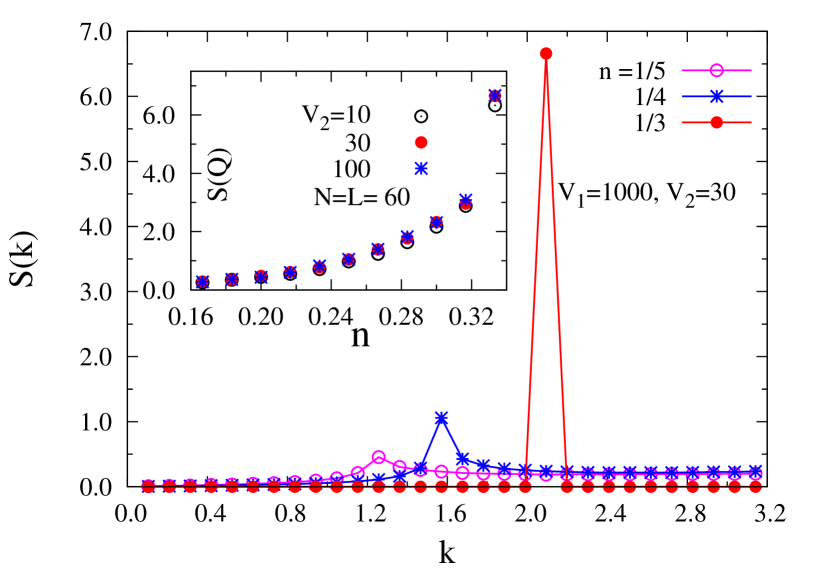
Figure 2: (Color online) WQMC plot of the structure factor $S(k)$ versus $k$ – for $N=L=60$, $\beta=L\Delta\tau$ with $\Delta\tau=0.125$, and at various densities – shows CDW at $n=1/3$ with $S(Q)\approx N/9$, i.e., maximum allowed value. The peak values $S(Q)$ rapidly fall as $n$ moves away from $1/3$ and are independent of $V_{2}$ at large values of $V_{2}$ [see inset].

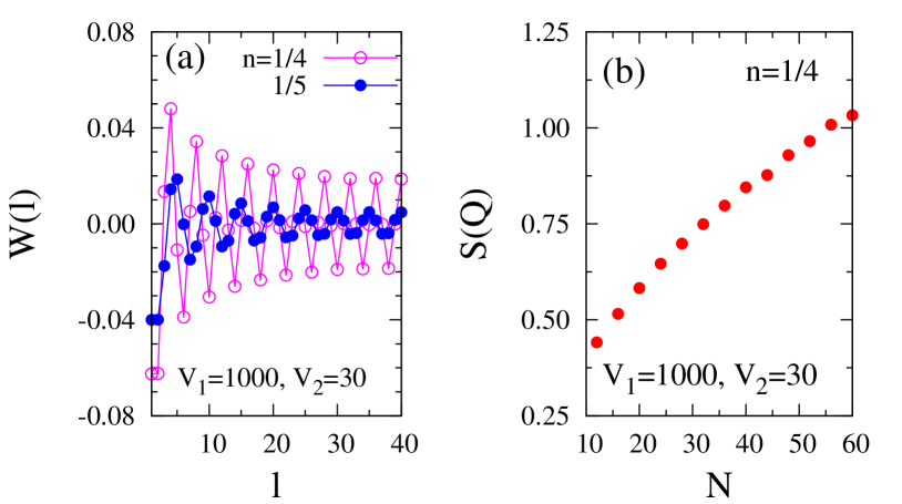
Figure 3: (Color online) Plots, obtained using WQMC at $\beta=N\Delta\tau$ with $\Delta\tau=0.125$, showing correlations in the $t$-$V_{1}$-$V_{2}$ model. The correlation function $W(l)$, plotted for $N=80$ sites in (a), does not seem to decay. The peak of the structure factor $S(Q)$, plotted in (b) for various system sizes at $n=1/4$, grows monotonically.

IV CDW correlations

The repulsive terms in the HCB Hamiltonian $H_{b}$ indicate that a CDW is possible. We study the correlations, by extending to our $t$-$V_{1}$-$V_{2}$ model, the well documented WQMC approach for obtaining correlation functions and structure factor for the $t$-$V$ model scalettar1 . Plots of the structure factor in Fig. 2 show a peak at wavevector $Q=2\pi n$ suggesting a CDW. However (as shown in Fig. 2), only at filling $n=1/3$, where the structure factor peak is approximately that for the strong CDW case corresponding to $V_{2}\rightarrow\infty$, can we assert that CDW occurs. Specifically at $n=1/3$ and for $V_{2}>10$, the $W(l)$ has a simple structure [i.e., $W(l)\approx 1/3-1/3\times 1/3=2/9$ when $l$ is a multiple of 3 whereas for other $l$ values $W(l)\approx-1/3\times 1/3=-1/9$] yielding $S(k)\approx\delta_{k,2\pi/3}N/9$. Furthermore (in Fig. 2), the peak of the structure factor $S(Q)$ (which remains essentially constant at all relevant interactions $V_{2}>10$) rapidly decreases as $n$ decreases from $1/3$ – a trend that is similar to that of $S(Q)$ for the $t$-$V$ model as one moves away from half-filling sdadys . Nevertheless, the plots of correlation function (in Fig. 3) do not seem to decay at large distance (for both $n=1/4$ and $n=1/5$) while the structure factor peak (for $n=1/4$) seems to grow monotonically with system size – all indicative of a CDW. Later on, the above ambivalence will be resolved and it will be demonstrated unequivocally that our $t$-$V_{1}$-$V_{2}$ model has a CDW only at $n=1/3$ while at other fillings $n<1/3$ superfluidity (and no CDW) results.

Since $V_{1}=\infty$ and because we are dealing with a one-dimensional system, we simplify the phase transition analysis by performing an exact mapping of the $N$-site $t$-$V_{1}$-$V_{2}$ model onto a $t$-$V$ model with $N-N_{p}$ sites and with $V=V_{2}$. This enables us to access bigger system sizes for performing numerics; furthermore, since the phase diagram of the $t$-$V$ model is well known, we can clearly determine the existence of a CDW which was not possible using the above structure-factor/correlation-function analysis. Later, we will also show that the $t$-$V$ model lends itself to a simple finite size scaling approach for obtaining accurately the superfluid density in the thermodynamic limit.

We first recognize that we can recast the HCB Hamiltonian in Eq. (16) as the following projected Hamiltonian $H_{b}^{P}$ where NN sites of a particle are projected out:

$$\!\!\!\!\!\!\!\!\!H_{b}^{P}= \!\sum\limits_{j}[-T\{(1-n_{j-1})b^{\dagger}_{j}b_{j+1}(1-n_{j+2})+{\rm H.c.}\}$$

$$~{}~{}~{}~{}+V_{2}(1-n_{j-1})n_{j}(1-n_{j+1})n_{j+2}(1-n_{j+3})]$$

$$= \!\sum\limits_{j}[-T(\tilde{b}^{\dagger}_{j}\tilde{b}_{j+1}+{\rm H.c.})+V_{2}\tilde{n}_{j}\tilde{n}_{j+2}].$$ (17)

where $\tilde{b}^{\dagger}_{j}\equiv(1-n_{j-1})b^{\dagger}_{j}(1-n_{j+1})$ and $\tilde{n}_{j}\equiv\tilde{b}^{\dagger}_{j}\tilde{b}_{j}$. Next, we observe that $H_{b}^{P}$ commutes with $\sum_{j}n_{j}(1-n_{j+1})$ and thus the total number of excitons (with each exciton comprising of a particle with a hole to its right) is conserved. Physically, this is due to the fact that infinite NN repulsion ensures that the neighboring sites of a particle are unoccupied. With each particle, we associate only one neighboring vacant site (say, the site on the right side of the particle) so that situations such as particles on NNN sites can also be dealt with. Then by deleting the sites of the holes in all the excitons and having only a NN interaction $V=V_{2}$ and no other interaction in the reduced system of $N_{1}\equiv N-N_{p}$ sites, we get the same eigenenergies (see Ref. dias, for a similar analysis for the $t$-$V$ model in one-dimension). We further recognize that there is a one-to-one mapping between the eigenstates of the $H_{b}^{P}$ Hamiltonian and the eigenstates of the $t$-$V$ Hamiltonian $H_{t-V}$,

$$H_{t-V}=\sum\limits_{j}[-T(b^{\dagger}_{j}b_{j+1}+{\rm H.c.})+Vn_{j}n_{j+1}],$$ (18)

with $V=V_{2}$ and $N_{1}$ sites while the corresponding eigenenergies are identical. We can thus extract the eigenenergy spectrum of the $t$-$V_{1}$-$V_{2}$ model by studying the equivalent $t$-$V$ model. We first observe that $n=N_{p}/N=1/3$ for the $t$-$V_{1}$-$V_{2}$ model corresponds to the $n=N_{p}/(N-N_{p})=1/2$ for the $t$-$V$ model and thus superfluid density vanishes (as the two models have the same eigenenergies) and a CDW results sdadys since the mass gap is the same for both. Furthermore, at all fractions $n<1/3$ for the $t$-$V_{1}$-$V_{2}$ model we get a superfluid (and no CDW) since for the $t$-$V$ model the same is true at $n<1/2$ sdadys . Lastly, since $n=1$ for the $t$-$V$ model translates to $n=1/2$ for the $t$-$V_{1}$-$V_{2}$ model, we note that electron-hole symmetry for the $t$-$V$ model guarantees that $t$-$V_{1}$-$V_{2}$ model exhibits superfluidity and absence of CDW for $1/3<n<1/2$ as well.

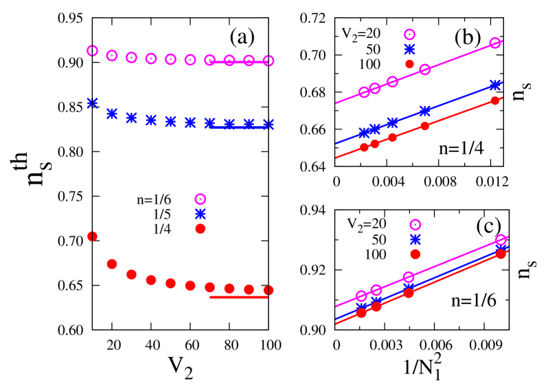
Figure 4: (Color online) Superfluid density for an infinite system $n_{s}^{th}$ at various densities $n$ and interactions $V_{2}$ for the $t$-$V_{1}$-$V_{2}$ model at $V_{1}=\infty$ are depicted in (a). Values of $n_{s}^{th}$ in (a) are the intercepts, obtained by extrapolation of the straight lines through the $n_{s}$ data plotted at various $1/N_{1}^{2}$ values, in figures such as (b) and (c). The solid lines in (a) are for $V_{2}=\infty$ and obtained from Eq. (20).

V Superfluid density

We will now substantiate the above observations on the occurrence of superfluidity through calculating the superfluid density by threading the chain with an infinitesimal magnetic flux. We will exploit the one-dimensionality of the system and outline a simple finite size scaling approach to calculate the superfluid density in the thermodynamic limit. We first note that the energy for the $t$-$V_{1}$-$V_{2}$ model, when $V_{2}=\infty$ and (as before) $V_{1}=\infty$, is given by the tight binding Hamiltonian energy for $N_{2}\equiv N-2N_{p}$ particles where we have excluded both the NN and NNN holes to the right of the particles in the $t$-$V_{1}$-$V_{2}$ model. The total energy, when threaded by a flux $\theta$, is expressed as

$$E(\theta)=-2T\sum\limits_{k}\cos[k+\theta/N_{2}].$$ (19)

Then the superfluid fraction is given by fisher ; sdsy1

$$\!\!\!\!\!\!\!\!n_{s}=\frac{N_{2}^{2}}{N_{p}T}\left[\frac{1}{2}\frac{\partial^{2}E}{\partial\theta^{2}}\right]_{\theta=0}=\frac{1}{N_{p}}\frac{\sin\left(\frac{\pi N_{p}}{N_{2}}\right)}{\sin\left(\frac{\pi}{N_{2}}\right)},$$ (20)

where anti-periodic (periodic) boundary conditions have been taken for even (odd) values of $N_{p}$. The superfluid density in the thermodynamic limit $n_{s}^{th}$ can be related to the finite ($N_{2}$-site) system superfluid density $n_{s}$ as follows:

$$n_{s}^{th}=n_{s}\left[1-\frac{1}{6}\left(\frac{\pi}{N_{2}}\right)^{2}+\frac{1}{120}\left(\frac{\pi}{N_{2}}\right)^{4}...\right].$$ (21)

From the above expression (valid for $V_{2}=\infty$), at a fixed density, we expect $(n_{s}^{th}-n_{s})/n_{s}\propto 1/N_{2}^{2}$ or $1/N_{1}^{2}$ (with corrections of order $1/N_{2}^{4}$ or $1/N_{1}^{4}$) for the large but finite $V_{2}$ case as well. We calculated the superfluid density at various large values of $V_{2}$, system sizes $N$, and filling fractions $n$; we find [as exemplified in Figs. 4(b) and 4(c)] that $n_{s}$ indeed varies linearly with $1/N_{1}^{2}$ using which we obtain the various $n_{s}^{th}$ values.

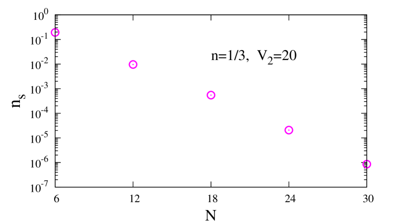
Figure 5: (Color online) Superfluid density decaying exponentially with system size for the CDW state at one-third filling and large NNN repulsion $V_{2}$.

From Fig. 4(a), we see that the superfluid density (plotted in the thermodynamic limit) gradually decreases with increasing $V_{2}$ and reaches the asymptotic value; the $n_{s}^{th}$ values for smaller filling fractions decrease more slowly because repulsion is less effective at lower densities. Regarding the superfluid density at $n=1/3$ and $V_{2}=\infty$, it vanishes at all system sizes as can be seen from Eq. (20). However, at finite $V_{2}\geq 10$, $n_{s}$ vanishes exponentially with system size [as shown in Fig. (5)] which is consistent with the fact that there is a full CDW gap at $n=1/3$.

VI BEC occupation number

Lastly, we will calculate the Bose-Einstein condensate (BEC) occupation number $n_{0}$. We first recall the well-established result that $n_{0}$, for a system of HCB in a one-dimensional tight binding lattice, varies as $C(n)\sqrt{N}$ in the thermodynamic limit with the coefficient $C(n)$ monotonically increasing from $0$ as the density $n$ increases from $0$ to $1/2$ lenard ; muramatsu1 ; consequently, the condensate fraction $n_{0}/N_{p}\propto 1/\sqrt{N}\rightarrow 0$. Next, in the presence of repulsion (as argued below), we expect the BEC occupation number $n_{0}$ to again scale as $\sqrt{N}$; however, the coefficient of $\sqrt{N}$ will be smaller due to the restriction on hopping imposed by repulsion.

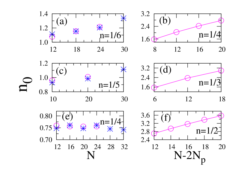
Figure 6: (Color online) Plots of BEC occupation number $n_{0}$, obtained from modified Lanczos (open circles) and WQMC (crosses), with (a), (c), and (e) pertaining to $t$-$V_{1}$-$V_{2}$ model (with $V_{1}=\infty$, and $V_{2}=35$) while (b), (d), and (f) respectively pertaining to the corresponding tight binding model with enhanced densities $N_{p}/(N-2N_{p})$. For WQMC, $\beta=N\Delta\tau$ with $\Delta\tau$ = 0.125, 0.15, and 0.175 for (a), (c), and (e) respectively.

The Bose-Einstein condensate (BEC) occupation number $n_{0}$ is obtained from

$$n_{0}=\frac{1}{N}\sum\limits_{i,j}\langle\Psi_{0}|b^{\dagger}_{i}b_{j}|\Psi_{0}\rangle,$$ (22)

where $|\Psi_{0}\rangle$ is the ground state. We calculate $n_{0}$ using two methods – modified Lanczos for smaller systems and a newly developed WQMC method for both small and larger systems (see Fig. 6). The values of $n_{0}$ for our $t$-$V_{1}$-$V_{2}$ model in a $N$-site original system $S_{O}$ at various densities [such as $n=1/4,1/5,1/6$] seem to be smaller than the $n_{0}$ for the corresponding transformed tight binding system $S_{2N_{p}}$, realized when $V_{1}=V_{2}=\infty$, with $N-2N_{p}$ sites and enhanced densities [$n/(1-2n)=1/2,1/3,1/4$, respectively]. This can be understood from the fact that, in the transformed $S_{2N_{p}}$ system of $N-2N_{p}$ sites [based on Eq. (22)], a particle can hop to more sites between two particles than in the original $t$-$V_{1}$-$V_{2}$ system leading to a larger $n_{0}$. For the $S_{2N_{p}}$ system, it is important to realize that $n_{0}\propto\sqrt{N-2N_{p}}\propto\sqrt{N}$.

We will now consider a tight binding system $S_{4N_{p}}$ with $N-4N_{p}$ sites and $N_{p}$ particles so as to obtain the lower bound for the BEC occupation number $n_{0}$ for the $N$-site $t-V_{1}-V_{2}$ system $S_{O}$. For every configuration in the $S_{4N_{p}}$ system, there is a corresponding configuration in the $S_{O}$ system that can be obtained by adding two empty sites to the right and two empty sites to the left of all particles. Furthermore, the ground state kinetic energy contribution of the $S_{4N_{p}}$ and $S_{2N_{p}}$ systems are both proportional to $N$; hence, in the ground state of the original $S_{O}$ system, the combined probability weighting of all the configurations obtained from the $S_{4N_{p}}$ system (by adding 4 empty sites next to every particle) is a finite fraction. Since the BEC occupation number $n_{0}$ of $S_{4N_{p}}$ system scales as $\sqrt{N}$, it follows that the lower bound of the $n_{0}$ for the original $S_{O}$ system also varies as $\sqrt{N}$. Thus, the BEC occupation number $n_{0}$ of the original $N$-site $t-V_{1}-V_{2}$ system $S_{O}$ will vary as $\sqrt{N}$ since it is constrained from above by $n_{0}\propto\sqrt{N}$ for the $S_{2N_{p}}$ system.

At higher densities (i.e., $1/3>n\geq 1/5$) in our $t$-$V_{1}$-$V_{2}$ model, we find that the values of $n_{0}$ seem to increase more slowly with system size [see Figs. 6(a), 6(c), and 6(e)] – this being due to smaller coefficients of $\sqrt{N}$ resulting from interaction effects. Moreover, we also note [from Figs. 6(b) and 6(e)] that the value of $n_{0}$ [i.e., the coefficient of $\sqrt{N}$ in the expression for $n_{0}$] decreases due to repulsion.

Our new WQMC method (see Appendix B for details) to obtain BEC fraction is a modification of the standard approach to studying correlations in the xxz model. scalettar1 ; scalapino Since the Hamiltonian is real, it can be shown that the probability amplitude of any basis state in the ground state expression can be taken as real and non-negative. Consequently, we approximate the ground state by

$$|\Psi\rangle=\sum\limits_{i}\sqrt{\frac{\langle\phi_{i}|\exp[-\beta H]|\phi_{i}\rangle}{Z}}~{}|\phi_{i}\rangle,$$ (23)

with $Z$ being the partition function, $|\phi_{i}\rangle$ a basis state of the system in the occupation number representation, and $\beta$ being sufficiently large. Then we calculate $n_{0}$ by setting $|\Psi_{0}\rangle=|\Psi\rangle$ in Eq. (22). Our WQMC approach to $n_{0}$ has been benchmarked against the modified Lanczos method for small system sizes (see Fig. 6). The number of passes needed to estimate $|\Psi\rangle$ turns out to be an order of magnitude larger than that needed for obtaining correlation functions by WQMC. We take $|\Psi\rangle$ to be the state that produces an estimate of the kinetic energy $\langle\Psi|K|\Psi\rangle$ (with $K$ being the kinetic energy operator) that is closest to the usual WQMC estimate $\langle\langle\phi_{i}|\exp[-\beta H]K|\phi_{i}\rangle/\langle\phi_{i}|\exp[-\beta H]|\phi_{i}\rangle\rangle_{\rm QMC}$ where $\langle\rangle_{\rm QMC}$ denotes a quantum Monte Carlo average over various states $|\phi_{i}\rangle$.

VII Conclusions

In this paper, we have analyzed the correlated NN singlet phase predicted by the effective Hamiltonian of the Hubbard-Holstein model by essentially mapping the Hamiltonian onto the well-understood one-dimensional $t$-$V$ model with large repulsion. Because the physics is dictated by the $t$-$V$ model, we find that CDW and superfluidity occur mutually exclusively with CDW resulting only at $n=1/3$ while superfluidity manifests itself at all other fillings. We also show that the the BEC occupation number $n_{0}$ for our model scales as $\sqrt{N}$ similar to the $n_{0}$ for a HCB tight binding model; additionally, we demonstrate numerically (using a new WQMC method and a modified Lanczos algorithm), at $n\neq 1/3$, that the $n_{0}$ for our model is smaller than the $n_{0}$ for a HCB tight binding model.

We close by observing that, while CDW and superconductivity seem to be incompatible in the one-dimensional HHM, experimental results (such as those reported in Refs. withers, ; chan, ; blanton, ) suggest that they can coexist in higher dimensions. Furthermore, the vanishing of BEC fraction for the HHM is again an artifact of the one-dimensionality and should make way to non-zero fractions for higher dimensions just as in the case of the xxz model sdsy1 .

VIII Acknowledgments

S. R. is supported by TCMP & CAMCS at Saha Institute of Nuclear Physics (India) and CCT & COT at Univ. of Cambridge (UK). P. B. L. is supported by the U.S. Department of Energy under Award No. FWP 70069.

Appendix A

In this appendix, we will outline our approach to carrying out perturbation theory and obtaining the ground state energy. We assume a Hamiltonian of the form $H=H_{0}+H_{1}$ where the unperturbed $H_{0}$ has separable eigenstates $|n,m\rangle=|n\rangle_{el}\otimes|m\rangle_{ph}$ with $|0,0\rangle$ being the ground state with zero phonons; the eigenenergies, corresponding to $|n,m\rangle$, are $E_{n,m}^{(0)}=E_{n}^{el}+E_{m}^{ph}$. Furthermore, the perturbation $H_{1}$ is the electron-phonon interaction term of the form given in Eq. (7).

After a canonical transformationsryspbl1 , we obtain

$$\tilde{H} = e^{S}He^{-S}$$ (24)

$$= \!\!H_{0}\!+\!H_{1}\!+\![H_{0}+H_{1},S]\!\!+\!\frac{1}{2}\left[[H_{0}\!+\!H_{1},S],S\right].$$

In the ground state energy, we know that the first-order perturbation term is zero by construction (in fact, $\langle n_{1},0|H_{1}|n_{2},0\rangle=0$). To eliminate the first-order term in $H_{1}$, we set $H_{1}+[H_{0},S]=0$. Consequently, we obtain the matrix elements

$$\langle n_{1},m_{1}|S|n_{2},m_{2}\rangle=-\frac{\langle n_{1},m_{1}|H_{1}|n_{2},m_{2}\rangle}{(E_{n_{1},m_{1}}-E_{n_{2},m_{2}})}.$$ (25)

We now assume that both NN hopping integral $te^{-g^{2}}$ and the Heisenberg spin interaction strength $J$ are much smaller compared to the phononic energy $\omega_{0}$ which is true at large couplings $g$. Hence, we make the approximation $(E_{n_{1},m_{1}}^{(0)}-E_{n_{2},m_{2}}^{(0)})\simeq(E_{m_{1}}^{ph}-E_{m_{2}}^{ph})$; then, using Eqs. (24) and (25), we obtain

$${{}_{ph}\!\langle m_{1}|\tilde{H}|m_{2}\rangle_{ph}}\simeq{{}_{ph}\!\langle m_{1}|H_{0}|m_{2}\rangle_{ph}}+\frac{1}{2}\sum_{\bar{m}}{{{}_{ph}\!\langle m_{1}|H_{1}|\bar{m}\rangle_{ph}}~{}{{}_{ph}\!\langle\bar{m}|H_{1}|m_{2}\rangle_{ph}}}\left[\frac{1}{E_{m_{2}}^{ph}-E_{\bar{m}}^{ph}}+\frac{1}{E_{m_{1}}^{ph}-E_{\bar{m}}^{ph}}\right].$$ (26)

Next, it is important to note that the second order correction $E^{(2)}_{n,m}$, corresponding to the unperturbed eigenenergy $E_{n,m}^{(0)}$, can be expressed as follows:

$$E^{(2)}_{n,m}=\sum_{\bar{m}}\frac{{\langle n,m|H_{1}|\bar{m}\rangle_{ph}}~{}{{}_{ph}\!\langle\bar{m}|H_{1}|n,m\rangle}}{{E_{m}^{ph}-E_{\bar{m}}^{ph}}}\simeq{\langle n,m|\tilde{H}|n,m\rangle}-{\langle n,m|H_{0}|n,m\rangle}.$$ (27)

Furthermore, since $\langle n_{1},0|H_{1}|n_{2},0\rangle=0$, $\langle n,0|\tilde{H}|n,0\rangle$ is the total energy that resulted from performing second order perturbation theory on the unperturbed energy $E_{n,0}^{(0)}$. Our procedure for finding ground state amounts to obtaining the lowest eigenvalue for the matrix with elements $\langle n_{1},0|\tilde{H}|n_{2},0\rangle$; this is equivalent to finding the ground state of the effective Hamiltonian $H_{e}$ (as was done in Ref. sryspbl1, ):

$$H_{e}={{}_{ph}\!\langle 0|H_{0}|0\rangle_{ph}}+H^{(2)},$$ (28)

where

$$H^{(2)}=\sum_{\bar{m}}\frac{{{}_{ph}\langle 0|H_{1}|\bar{m}\rangle_{ph}}\times{{}_{ph}\!\langle\bar{m}|H_{1}|0\rangle_{ph}}}{{E_{0}^{ph}-E_{\bar{m}}^{ph}}}.$$ (29)

This procedure amounts to considering the restricted subspace spanned by eigenstates $|n,0\rangle_{1}$ obtained from carrying out first order perturbation theory on $|n,0\rangle$:

$$|n,0\rangle_{1}=|n,0\rangle+\sum_{\bar{m}}\frac{{|\bar{m}\rangle_{ph}}~{}{{}_{ph}\!\langle\bar{m}|H_{1}|n,0\rangle}}{{E_{0}^{ph}-E_{\bar{m}}^{ph}}},$$ (30)

It is important to recognize that the state $|n,0\rangle_{1}$ is not separable, i.e., cannot be expressed as a product of an electronic wavefunction and a phononic wavefunction. We have restricted ourselves to the subspace of the states $|n,0\rangle_{1}$ because the states $|n,m\neq 0\rangle_{1}$ correspond to higher energy states due to the fact that the electronic excitation energy is much smaller than the phononic energy, i.e., $te^{-g^{2}}<<\omega_{0}$. Additionally, we would like to point out that the total ground state energy (in second order perturbation theory) is obtained by diagonalizing the matrix whose elements are $\langle n_{1},0|H|n_{2},0\rangle_{1}$.

Appendix B WQMC FOR BEC FRACTION

We will discuss, in brief, the usual world-line quantum Monte Carlo (WQMC) approach scalettar1 ; scalapino adapted for calculating correlations in our $t$-$V_{1}$-$V_{2}$ model Hamiltonian given below:

$$H_{b}=\!\sum\limits_{j}{H^{j}} = \sum\limits_{j}[-T(b^{\dagger}_{j}b_{j+1}+{\rm H.c.})$$ (31)

$$+ V_{1}n_{j}n_{j+1}+V_{2}n_{j}n_{j+2}].$$

Since this is quite similar to the $t$-$V$ model, we can employ the checkerboard decomposition $H_{b}=H_{1}+H_{2}$ where $H_{1}=\!\sum\limits_{j~{}{\rm odd}}H^{j}$ and $H_{2}=\!\sum\limits_{j~{}{\rm even}}H^{j}$. It is important to note that both $H_{1}$ and $H_{2}$ consist of independent two-site pieces. Because of the decomposition, it becomes easier to evaluate the expectation value of an operator $A$ given by

$$\langle A\rangle=\frac{Tr[Ae^{-\beta H_{b}}]}{Tr[e^{-\beta H_{b}}]},$$ (32)

with $A$ involving only number operators (such as $n_{i}n_{j}$) or NN hopping operators (such as $b^{\dagger}_{j}b_{j+1}+{\rm H.c.}$). Now we calculate the partition function:

$$Z = Tr[e^{-\beta H_{b}}]$$

$$= \sum\limits_{i_{1},...,i_{2L}}\!\!\!\!\langle i_{1}|U_{1}|i_{2L}\rangle\langle i_{2L}|U_{2}|i_{2L-1}\rangle...{\langle i_{3}|U_{1}|i_{2}\rangle}\langle i_{2}|U_{2}|i_{1}\rangle.$$

Here $U_{i}=e^{-\Delta\tau H_{i}},\beta=L\Delta\tau$, and each of $|i_{1}\rangle$, …,$|i_{2L}\rangle$ form a complete basis set in the occupation number representation. Here the world lines are the locus of the particles in the imaginary time ($\tau$) direction.

For the density-density correlation function $\langle n_{i}n_{i+l}\rangle$ (which is the expectation value of a diagonal operator), the above procedure of inserting $2L$ time slices yields the simple form

$$\langle n_{i}n_{i+l}\rangle=\frac{1}{2}\left\langle[\langle i_{L}|n_{i}n_{i+l}|i_{L}\rangle+\langle i_{L+1}|n_{i}n_{i+l}|i_{L+1}\rangle]\right\rangle_{\rm QMC},$$

where $\langle\hskip 8.53581pt\rangle_{QMC}$ represents average over many QMC passes. Notice that we have concentrated only on $L$ and $L+1$ time slice indexes although expectation value can be taken over all the $2L$ time slice indexes for better statistics. As for $\langle b^{\dagger}_{j}b_{j+1}+{\rm H.c.}\rangle$ (which corresponds to a non-diagonal operator), WQMC procedure yields

$$\langle b^{\dagger}_{j}b_{j+1}+{\rm H.c.}\rangle=\langle\frac{\langle i_{M}|(b^{\dagger}_{j}b_{j+1}+{\rm H.c.})U_{k}|i_{M+1}\rangle}{\langle i_{M}|U_{k}|i_{M+1}\rangle}\rangle_{\rm QMC},$$

where, for odd (even) values of $j$, we take $k=1$ ($2$) and even (odd) $M$. However, as regards obtaining expectation value of $(b^{\dagger}_{j}b_{j+m}+{\rm H.c.})$ for $m>1$, the simple procedure (involving checkerboard decomposition) given above is not applicable; moreover, other suggested procedures in the literature are complicated scalettar1 .

Here, we propose an alternate simple method for evaluating $\langle b^{\dagger}_{j}b_{j+m}+{\rm H.c.}\rangle$ for $m>1$ and thus obtaining the BEC occupation number

$$n_{0}=\frac{1}{N}\sum\limits_{i,j}\langle\Psi_{0}|b^{\dagger}_{i}b_{j}|\Psi_{0}\rangle,$$ (33)

with $|\Psi_{0}\rangle$ being the ground state. To the WQMC method mentioned above, we add our trick to construct $|\Psi_{0}\rangle$ as a linear combination of the basis states $|\phi_{i}\rangle$ in the occupation number representation, i.e., $|\Psi_{0}\rangle=\sum\limits_{i}a_{i}|\phi_{i}\rangle$ with $\sum\limits_{i}a_{i}^{2}=1$. Once we get a good estimate of the ground state $|\Psi_{0}\rangle$, we can calculate the expectation values of any operator.

After equilibrium (which is attained after several QMC passes), we run the simulation for a sufficient number of QMC passes and store the basis states corresponding to time slices $L$ and $L+1$ in each pass. It is obvious that some of the basis states will occur more frequently. The frequency of occurrence of a basis state $|\phi_{i}\rangle$ is proportional to the probability ($a_{i}^{2}$) of its occurrence in the expansion of the ground state $|\Psi_{0}\rangle$. Now, the coefficients $a_{i}$ can be taken as real because the Hamiltonian is real and consequently $|\Psi_{0}\rangle$ can also be taken as real. Furthermore, all $a_{i}$ can be taken to be positive for the following reason. Firstly, the expectation values of NN and NNN interaction terms remain unaffected by the sign of $a_{i}$ . Next, the expectation value of the hopping term is given by

$$-T\langle\Psi_{0}|b_{l}^{\dagger}b_{l+1}|\Psi_{0}\rangle = -T\sum\limits_{i,j}\langle\phi_{i}|a_{i}(b_{l}^{\dagger}b_{l+1})a_{j}|\phi_{j}\rangle]$$ (34)

$$= -T\sum\limits_{i,k}\langle\phi_{i}|a_{i}c_{k}|\phi_{k}\rangle]$$

$$= -T\sum\limits_{i}a_{i}c_{i}.$$

This value is minimized when $a_{i}$ and $c_{i}$ have the same sign. Then, if we take $a_{i}$ to be positive for all $i$, $c_{i}>0$ for all $i$. Thus in $|\Psi_{0}\rangle=\sum\limits_{i}a_{i}|\phi_{i}\rangle$, we can take all $a_{i}$ to be positive and real.

Let $|\Psi_{i}\rangle$ and $E_{i}$ be the eigenstates and the eigenenergies of the Hamiltonian with $E_{0}$ being the ground state energy. For sufficiently large $\beta$, we approximate the ground state by

$$|\Psi\rangle = \sum\limits_{i}\sqrt{\frac{\langle\phi_{i}|\exp[-\beta H]|\phi_{i}\rangle}{Z}}~{}|\phi_{i}\rangle,$$ (35)

because then

$$|\Psi\rangle = \sum\limits_{i}\sqrt{\frac{\langle\phi_{i}|\sum_{j}|\Psi_{j}\rangle\langle\Psi_{j}|\exp[-\beta H]\sum_{k}|\Psi_{k}\rangle\langle\Psi_{k}||\phi_{i}\rangle}{Z}}~{}|\phi_{i}\rangle$$ (36)

$$\approx \sum\limits_{i}\sqrt{\frac{\langle\phi_{i}|\Psi_{0}\rangle\exp[-\beta E_{0}]\langle\Psi_{0}|\phi_{i}\rangle}{Z}}~{}|\phi_{i}\rangle$$

$$\approx \sum_{i}\langle\phi_{i}|\Psi_{0}\rangle|\phi_{i}\rangle=|\Psi_{0}\rangle,$$

since the partition function $Z=\sum_{i}\langle\Psi_{i}|\exp[-\beta H]|\Psi_{i}\rangle\approx\exp[-\beta E_{0}]$.

References

- (1) For a review, see R. L. Withers and J. A. Wilson, J. Phys. C 19, 4809 (1986).
- (2) E. Kim and M. H. W. Chan, Nature 427, 225 (2004); Science 305, 1941 (2004).
- (3) S. H. Blanton, R. T. Collins, K. H. Kelleher, L. D. Rotter, Z. Schlesinger, D. G. Hinks, and Y. Zheng, Phys. Rev. B 47, 996 (1993).
- (4) W. W. Fuller, P. M. Chaikin, and N. P. Ong, Phys. Rev. B 24, 1333 (͑1981).
- (5) A. Rusydi, W. Ku, B. Schulz, R. Rauer, I. Mahns, D. Qi, X. Gao, A. T. S. Wee, P. Abbamonte, H. Eisaki, Y. Fujimaki, S. Uchida, and M. Rübhausen, Phys. Rev. Lett. 105, 026402 (2010); P. Abbamonte, G. Blumberg, A. Rusydi, A. Gozar, P. G. Evans, T. Siegrist, L. Venema, H. Eisaki, E. D. Isaacs, and G. A. Sawatzky, Nature (London) 431, 1078 (2004).
- (6) H. Mori, I. Hirabayashi, S. Tanaka, T. Mori, Y. Maruyama, and H. Inokuchi, Solid State Commun. 80, 411 (1991).
- (7) J. Merino and R. H. McKenzie, Phys. Rev. Lett. 87, 237002 (͑2001).
- (8) K. Kudo, Y. Nishikubo, M. Nohara, J. Phys. Soc. Jpn. 79, 123710 (2010).
- (9) A. Lanzara, P. V. Bogdanov, X. J. Zhou, S. A. Kellar, D. L. Feng, E. D. Lu, T. Yoshida, H. Eisaki, A. Fujimori, K. Kishio, J.-I. Shimoyama, T. Noda, S. Uchida, Z. Hussain, and Z. X. Shen, Nature (London) 412, 510 (2001).
- (10) G.-H. Gweon, T. Sasagawa, S. Y. Zhou, J. Graf, H. Takagi, D.-H. Lee, and A. Lanzara, Nature (London) 430, 187 (2004).
- (11) A. Lanzara, N. L. Saini, M. Brunelli, F. Natali, A. Bianconi, P. G. Radaelli, and S.-W. Cheong Phys. Rev. Lett. 81, 878 (1998).
- (12) A. J. Millis, P. B. Littlewood, and B. I. Shraiman, Phys. Rev. Lett. 74, 5144 (1995).
- (13) F. Massee, S. de Jong, Y. Huang, W. K. Siu, I. Santoso, A. Mans, A. T. Boothroyd, D. Prabhakaran, R. Follath, A. Varykhalov, L. Patthey, M. Shi, J. B. Goedkoop, and M. S. Golden, Nat. Phys. 7, 978 (2011).
- (14) O. Gunnarsson, Rev. Mod. Phys. 69, 575 (1997).
- (15) S. Reja, S. Yarlagadda, and P. B. Littlewood, Phys. Rev. B 84, 085127 (2011).
- (16) A. Dobry, A. Greco, J. Lorenzana, and J. Riera, Phys. Rev. B 49, 505 (͑1994͒).
- (17) A. Dobry, A. Greco, J. Lorenzana, J. Riera, and H. T. Diep, Europhys. Lett. 27, 617 (͑1994͒).
- (18) B. Bäuml, G. Wellein, and H. Fehske, Phys. Rev. B 58, 3663 ͑(1998͒).
- (19) M. Tezuka, R. Arita, and H. Aoki, Phys. Rev. B 76, 155114 (2007).
- (20) Shigetoshi Sota and Takami Tohyama, Phys. Rev. B 82, 195130 (2010).
- (21) J. E. Hirsch and E. Fradkin, Phys. Rev. B 27, 4302 (͑1983͒).
- (22) J. E. Hirsch, Phys. Rev. B 31, 6022 (͑1985͒).
- (23) E. Berger, P. Valášek, and W. von der Linden, Phys. Rev. B 52, 4806 (͑1995͒).
- (24) Z. B. Huang, W. Hanke, E. Arrigoni, and D. J. Scalapino, Phys. Rev. B 68, 220507(R)͑ (2003͒).
- (25) R. P. Hardikar and R. T. Clay, Phys. Rev. B 75, 245103 (2007).
- (26) A. Macridin, G. A. Sawatzky, and M. Jarrell, Phys. Rev. B 69, 245111 (2004).
- (27) M. Grilli and C. Castellani, Phys. Rev. B 50, 16880 (͑1994͒).
- (28) J. Keller, C. E. Leal, and F. Forsthofer, Physica B 206-207, 739 (͑1995͒).
- (29) E. Koch and R. Zeyher, Phys. Rev. B 70, 094510 (͑2004͒).
- (30) U. Trapper, H. Fehske, M. Deeg, and H. Buttner, Z. Phys. B: Condens. Matter 93, 465 (1994).
- (31) C. A. Perroni, V. Cataudella, G. De Filippis, and V. Marigliano Ramaglia, Phys. Rev. B 71, 113107 (2005).
- (32) J. K. Freericks and M. Jarrell, Phys. Rev. Lett. 75, 2570 (͑1995͒).
- (33) M. Capone, G. Sangiovanni, C. Castellani, C. Di Castro, and M. Grilli, Phys. Rev. Lett. 92, 106401 (͑2004͒).
- (34) W. Koller, D. Meyer, Y. Ōno, and A. C. Hewson, Europhys. Lett. 66, 559 (͑2004͒).
- (35) W. Koller, D. Meyer, and A. C. Hewson, Phys. Rev. B 70, 155103 (͑2004͒).
- (36) G. S. Jeon, T.-H. Park, J. H. Han, H. C. Lee, and H.-Y. Choi, Phys. Rev. B 70, 125114 (͑2004͒).
- (37) G. Sangiovanni, M. Capone, C. Castellani, and M. Grilli, Phys. Rev. Lett. 94, 026401 (͑2005͒).
- (38) G. Sangiovanni, M. Capone, and C. Castellani, Phys. Rev. B 73, 165123 (͑2006͒).
- (39) J. Bauer and A. C. Hewson Phys. Rev. B 81, 235113 (2010).
- (40) Johannes Bauer and Giorgio Sangiovanni, Phys. Rev. B 82, 184535 (2010).
- (41) R. Zeyher and M. L. Kulić, Phys. Rev. B 53, 2850 (͑1996͒).
- (42) Y. Takada and A. Chatterjee, Phys. Rev. B 67, 081102 (͑2003).
- (43) H. Fehske, D. Ihle, J. Loos, U. Trapper, and H. Buttner, Z. Phys. B: Condens. Matter 94, 91 (1994).
- (44) A. Di Ciolo, J. Lorenzana, M. Grilli, and G. Seibold, Phys. Rev. B 79, 085101 (͑2009).
- (45) P. Barone, R. Raimondi, M. Capone, C. Castellani, and M. Fabrizio, Phys. Rev. B 77, 235115 (2008).
- (46) Alexandre Payeur and David Sénéchal, Phys. Rev. B 83, 033104 (2011).
- (47) E. R. Gagliano, E. Dagotto, A. Moreo, and F. C. Alcaraz, Phys. Rev. B 34, 1677 (1986͒); ibid. 35, 5297 (͑1987͒).
- (48) A. S. Alexandrov and N. F. Mott, Polarons and Bipolarons (World Scientific, Singapore, 1995).
- (49) E. V. L. de Mello and J. Ranninger, Phys. Rev. B 58, 9098 (1998); B. K. Chakraverty, J. Ranninger, and D. Feinberg, Phys. Rev. Lett. 81, 433 (1998).
- (50) R. T. Clay and R. P. Hardikar Phys. Rev. Lett. 95, 096401 (2005); R. P. Hardikar and R. T. Clay, Phys. Rev. B 75, 245103 (2007).
- (51) J. Bonc̆a, T. Katras̆nik, and S. A. Trugman, Phys. Rev. Lett. 84, 3153 (2000).
- (52) H. Eskes and R. Eder, Phys. Rev. B 54, 14226 (1996).
- (53) B. Ammon, M. Troyer, and H. Tsunetsugu, Phys. Rev. B, 52, 629 (1995).
- (54) A. P. Balachandran, E. Ercolessi, G. Morandi, and A. M. Srivastava, Int. J. Mod. Phys. B, 4, 2057 (1990).
- (55) I. G. Lang and Yu. A. Firsov, Zh. Eksp. Teor. Fiz. 43, 1843 (1962) [Sov. Phys. JETP 16, 1301 (1963)].
- (56) R. Pankaj and S. Yarlagadda, Phys. Rev. B 86, 035453 (2012).
- (57) The phase diagram results for are qualitatively similar to those for .
- (58) R. T. Scalettar, in Quantum Monte Carlo Methods in Physics and Chemistry, NATO Science Series, Series C: Mathematical and Physical Sciences Vol. 525, edited by M. P. Nightingale and Cyrus J. Umrigar (͑Kluwer Academic Publishers, Boston, 1999͒).
- (59) S. Datta, A. Das, and S. Yarlagadda, Phys. Rev. B 71, 235118 (2005); F. D. M. Haldane, Phys. Rev. Lett. 45, 1358 (͑1980͒).
- (60) R. G. Dias, Phys. Rev. B 62, 7791 (2000).
- (61) M. E. Fisher, M. N. Barber, and D. Jasnow, Phys. Rev. A 8, 1111 (1973).
- (62) S. Datta and S. Yarlagadda, Solid State Commun. 150 , 2040 (2010).
- (63) A. Lenard, J. Math. Phys. 5, 930 (͑1964).
- (64) M. Rigol and A. Muramatsu, Phys. Rev. A 72, 013604 (2005).
- (65) J. E. Hirsch, R. L. Sugar, D. J. Scalapino, and R. Blankenbecler, Phys. Rev. B 26, 5033 (1982).