We analyze the thermalization properties and the validity of the Eigenstate Thermalization Hypothesis in a generic class of quantum Hamiltonians where the quench parameter explicitly breaks a $Z_{2}$ symmetry. Natural realizations of such systems are given by random matrices expressed in a block form where the terms responsible for the quench dynamics are the off-diagonal blocks. Our analysis examines both dense and sparse random matrix realizations of the Hamiltonians and the observables. Sparse random matrices may be associated with local quantum Hamiltonians and they show a different spread of the observables on the energy eigenstates with respect to the dense ones. In particular, the numerical data seems to support the existence of rare states, i.e. states where the observables take expectation values which are different compared to the typical ones sampled by the micro-canonical distribution. In the case of sparse random matrices we also extract the finite size behavior of two different time scales associated with the thermalization process.

1 Introduction

Largely triggered by recent experiments on cold atoms [1, 2, 3, 4, 5], there has been in the past few years intense theoretical activity aimed at understanding the non-equilibrium dynamics in closed interacting quantum systems following a change in one of the system parameters. In many interesting cases, the system parameters can be changed rapidly with respect to all other time scales of the system that it is meaningful to consider the limit known as a quantum quench: namely, the system is prepared in an energy eigenstate $|\psi_{0}\rangle$ of an initial pre-quench Hamiltonian, $H_{pre}$, and then is allowed to evolve according to a new post-quench Hamiltonian, $H_{post}$, which differs from $H_{pre}$ by some variation of a parameter. Given that such a time evolution is purely unitary, one may wonder whether the system reaches, for large times, a new steady state and, moreover, if measurements done on this state are able to be related to the thermal density matrix of the system.

Recent progress in understanding thermalization of an extended quantum system following a quench has involved both analytical and numerical studies. From the analytical point of view, one of the first results can be traced back to von Neumann [6] (see also [7]), who pointed out the subtleties involved in defining a quantum generalization of the notion of ergodicity. Imagine, for example, that with an appropriate choice of the pre-quench Hamiltonian, $H_{pre}$, we have prepared the system in a linear superposition of ${\mathcal{N}}$ energy eigenstates, $|E_{a}\rangle$, of the post-quench Hamiltonian $H_{post}$, all in a shell of energies, $|E_{a}-\overline{E}|<\Delta$, centered at $\overline{E}$:

$$|\Psi\rangle\,=\,\sum_{|E_{a}-\overline{E}|<\Delta}c_{a}|E_{a}\rangle\,\,\,.$$ (1.1 )

The time average of the density matrix based on this state, given by

$$\rho_{diag}(\overline{E})\,=\,\overline{|\Psi(t)\rangle\langle\Psi(t)|}\,=\,\sum_{|E_{a}-\overline{E}|<\Delta}|c_{a}|^{2}|E_{a}\rangle\langle E_{a}|\,\,\,,$$ (1.2 )

defines the so-called diagonal ensemble which is, in general, different from the micro-canonical density matrix defined by

$$\rho_{mc}(\overline{E})\,=\,\frac{1}{{\mathcal{N}}}\sum_{|E_{a}-\overline{E}|<\Delta}|E_{a}\rangle\langle E_{a}|\,\,\,.$$ (1.3 )

So, unless it happens that $|c_{a}|^{2}=1/{\mathcal{N}}$, quantum ergodicity is strictly speaking almost never realized. Things may be however different if one looks at the long time evolution (and time average) of the expectation value of macroscopic observables, ${\mathcal{O}}$. For these quantities, defining $\langle{\mathcal{O}}\rangle_{diag}=\rm{Tr}({\mathcal{O}}\rho_{diag}(\overline{E}))$ and $\langle{\mathcal{O}}\rangle_{mc}=\rm{Tr}({\mathcal{O}}\rho_{mc}(\overline{E}))$, it may be true that the identity

$$\overline{\langle\Psi(t)|{\mathcal{O}}|\Psi(t)\rangle}\,=\,\langle{\mathcal{O}}\rangle_{diag}=\langle{\mathcal{O}}\rangle_{mc}\,\,\,,$$ (1.4 )

indeed holds. One possibility is that the expectation values ${\mathcal{O}}_{aa}=\langle E_{a}|{\mathcal{O}}|E_{a}\rangle$ of the macroscopic observables do not fluctuate between the Hamiltonian eigenstates which are close in energy. In this case, in fact, the identity (1.4) holds for all those initial states which are sufficiently narrow in energy. This is, in a nutshell, the scenario known in the literature as the Eigenstate Thermalization Hypothesis (ETH)) which was put forward by Deutsch and Srednicki [8, 9], based on previous work by Berry [10], and which has been recently advocated by Rigol et al. [11] as the mechanism behind the thermalization processes in quantum extended systems.

Recently this hypothesis has been put under intense scrutiny by different groups. The main emphasis heretofore has been given to the numerical analysis of specific models, such as hard-core bosons [11, 25], the Bose-Hubbard model [26], strongly correlated interacting fermions [27], the Hubbard model [28], one dimensional spin chains [17], etc. In this paper, instead of analyzing a particular system, we take a different approach. Namely, our strategy herein is to study the thermalization properties of a generic class of Hamiltonians and a generic set of observables. The natural language to approach the problem from this point of view is obviously provided by random matrices [29], which in the following will parametrize both the Hamiltonians and the observables. In particular we have chosen to study the quantum quenches and the relative thermalization in a class of Hamiltonians given by

$$H(h)=H_{0}+hV\,\,\,,$$ (1.5 )

where the quench parameter $h$ is meant to explicitly break a $Z_{2}$ symmetry of the ’unperturbed’ Hamiltonian $H_{0}$. Such Hamiltonians, which are arguably among the simplest examples of quantum systems, may model spin chains in the presence of an external magnetic field but, as we shall see later, they may also encode the familiar quantum Ising chain in a transverse magnetic field. Given the relative simplicity of this class of Hamiltonians, studying their quench dynamics may be a useful path to extract interesting information on generic properties of non-equilibrium systems, thus disregarding, in doing so, all additional complications coming from a richer structure of states of a specific model.

However, even upon adopting the abstract language of random matrices, an important issue governing thermalization properties and of which to be mindful is the locality of the interaction. Indeed, the mechanism behind thermalization may be different in the case in which the Hamiltonian is local and when it is not. As argued below, local Hamiltonians and local observables are associated to sparse matrices, i.e. matrices with a small proportion of non-zero entries, while non-local Hamiltonians and non-local observables are described by dense matrices. The two kinds of matrices have two different densities of states and it is essentially for this reason that one observes a different behavior of the eigenstates under a quench of the parameter $h$.

Important features of quantum quench processes in local systems were discussed in a paper by Biroli et al. [32], in particular the role played by rare fluctuations in the thermalization of local observables. These authors considered the existence of certain rare eigenstates – rare compared to the typical ones sampled by the micro-canonical distribution – but which may be responsible, if properly weighted, for the absence of thermalization observed in certain systems. As discussed in more detail later, the presence of such states can be detected by studying the spread of the expectation values of the observables on the energy eigenstates, in particular by the finite size dependence of the distribution of expectation values. The numerical analysis that we have performed seems indeed to indicate the existence of these rare states in the case of sparse random matrices, while they are absent in the case of dense random matrices. However, in our numerics, thermalization is observed nonetheless in sparse matrix Hamiltonians, simply because our averaging procedure on the different sampling of observables and Hamiltonians does not place a natural exponentially large weight upon the rare states, thus enabling them to break thermalization.

It should be underlined that the existence of rare states in the thermodynamic limit has been debated in the literature and in particular in a series of papers by Santos and Rigol [33, 34, 35]. They have argued that in a portion of the phase diagram of an extended t-J model with next-nearest-neighbour interactions, rare states are absent. We will come back to this conclusion in our presentation of results.

The paper is organized as follows: in Section 2 we discuss the notion of locality in regards to a Hamiltonian for a quantum system, and we argue that the corresponding matrix representation is given by a sparse matrix. We follow this in Appendix A with an extended discussion of whether a matrix sparse in a position basis is also sparse in the corresponding momentum basis. In Section 3 we address the issue of the ETH and, following Ref. [32], we briefly remind the reader of certain salient issues regarding the application of the ETH to our quenches. Section 4 is devoted to the discussion of our quench protocol implemented on $Z_{2}$ breaking quantum Hamiltonians. Section 5 deals with this protocol as applied to dense random matrices, while Section 6 treats sparse random matrices. In Section 7 we discuss the relevant time scales for thermalization in sparse random matrices, while our conclusions are presented in Section 8.

2 Locality

In this section we discuss the nature of Hamiltonian matrices associated with local models. In order to consider finite-size matrices, we will always have in mind that the model contains (effectively) proper physical cut-offs (for example, volume or lattice spacings) such that the Hilbert space involved is actually finite. For local models here we mean models local in the space variable, ${\bf x}$, (if continuous) or in the lattice site, ${\bf i}$, if discrete. The main idea of this section is the following: in a generic basis of the Hilbert space, the matrix representation of a local Hamiltonian corresponds to a dense matrix, i.e. a matrix which has all entries different from zero (an explicit example will be given below). However, if the theory is local, there will exist a basis (in the following called the local basis), in which the Hamiltonian will be represented by a sparse matrix, i.e. a matrix where the great majority of its entries are zero. In the following, for simplicity, we focus our attention on one-dimensional systems.

2.1 Local basis

To clarify the concept of the local basis, it is worth starting our discussion by a paradigmatic example: the 1d quantum Ising model in a longitudinal field (generically a non-integrable model). In this case the quantum Hamiltonian for $L$ sites is given in terms of Pauli matrices and takes the form:

$$H\equiv\sum_{i=1}^{L}\sigma^{z}_{i}\sigma^{z}_{i+1}+h\sigma^{x}_{i}+\sigma^{z}_{i}=\sum_{i=1}^{L}H_{i}.$$ (2.1 )

The last equality makes evident the local nature of this model: the Hamiltonian has been written as a sum of operators involving only two lattice sites. The matrix representation can be obtained once we fix a basis. A typical choice is given by the set of common eigenstates of the $\sigma^{z}_{i}$ operators. They can be written as,

$$|\uparrow\uparrow\ldots\uparrow\rangle,\quad|\uparrow\uparrow\ldots\downarrow\rangle,\ldots\quad\Rightarrow\quad|m_{1}m_{2}\ldots m_{L}\rangle,$$ (2.2 )

where each $m_{i}\in\{\uparrow,\downarrow\}$ corresponds to the two possible eigenstates of $\sigma^{z}_{i}$:

$$\sigma^{z}_{i}|\uparrow\rangle=|\uparrow\rangle,\quad\sigma^{z}_{i}|\downarrow\rangle=-|\downarrow\rangle\quad\Rightarrow\quad\sigma_{z}^{i}|m_{i}\rangle=m_{i}|m_{i}\rangle.$$

Therefore the Hilbert space is made of $N=2^{L}$ elements. We call this the real-space basis and it can be characterized by the fact that its elements are tensor products of the states of each site. Now let’s consider the matrix element of the Hamiltonian density $H_{i}$:

$$H_{i}^{s,s^{\prime}}=\langle m_{1}\ldots m_{N}|H_{i}|m_{1}^{\prime}\ldots m_{N}^{\prime}\rangle=((m_{i}m_{i+1}+m_{i})\delta_{m_{i},m_{i}^{\prime}}+h\delta_{m_{i},-m_{i}^{\prime}})\prod_{k\neq i}\delta_{m_{k},m_{k}^{\prime}},$$ (2.3 )

where $s,s^{\prime}$ are shorthand for the full set of indices, $m_{1},\ldots,m_{N}$. From this expression it is easy to deduce that on each row of the matrix there are $L+1$ non-zero entries and therefore the total number of non-zero elements of the $N\times N$ matrix $H$ is ${\mathcal{N}}=(L+1)N$. Since the total number of matrix elements is $N^{2}$, the density of non-zero elements is given by

$$\rho\,=\,\frac{{\mathcal{N}}}{N^{2}}\,=\,\left(\frac{\ln N}{\ln 2}+1\right)\frac{1}{N}\propto\frac{\ln N}{N}\,\,\,,$$ (2.4 )

while the density of the zeros of the matrix $H$ is

$$\rho_{0}\,=\,1-\rho\,\simeq\,1-\frac{k\ln N}{N}.$$ (2.5 )

The constant $k$ is related to specific properties of the model, but the scaling in Eq. (2.4) is general. Therefore for large values of $N$, the Hamiltonian matrix $H_{N}$ is a sparse matrix, i.e. a matrix with a large number of zeros and few non-zero entries. This statement holds in general for any local quantum Hamiltonian, as for instance the one coming from a quantum field theory: the fraction of non-zero elements of the Hamiltonian is exponentially suppressed in the thermodynamic limit $L\rightarrow\infty$. Take for instance a $(1+1)$ bosonic field theory, whose Hamiltonian can be written as

$$H\,=\,\int{\mathcal{H}}(x)\,dx\,=\,\int\left[\frac{1}{2}\Pi^{2}(x,t)+\frac{1}{2}(\partial_{x}\hat{\varphi}(x,t))^{2}+V(\hat{\varphi}(x,t))\right]\,dx\,\,\,,$$ (2.6 )

where $\Pi(x,t)=\frac{\partial\hat{\varphi}}{\partial t}$ is the canonical conjugate of the operator $\hat{\varphi}(x,t)$ entering the equal-time commutation relation,

$$[\hat{\varphi}(x,t),\Pi(y,t)]\,=\,i\delta(x-y)\,\,\,.$$ (2.7 )

Once the space coordinate $x$ and the field values have been discretized, we can choose the basis of eigenstates of the operators $\varphi_{x_{i}}$ and the Hamiltonian (2.6) can be expressed as a matrix. All the terms except the momentum become diagonal in this basis. The momentum instead plays the same role of a "spin flip" operator as $\sigma^{x}$ does in the Ising case: one can easily see that this term provides off-diagonal coefficients in the matrix, and in each row they will be as many non-zero entries as there are lattice sites. Therefore a scaling analogous to Eq. (2.5) is found.

2.2 The basis of momenta

In the last section we pointed out the kind of matrices one should expect when a local model is formulated in a real-space basis. However one can ask the question what happens to the sparseness of the matrix if the basis is changed. Among all other possible bases, it is the momentum basis that is often used to express the Hamiltonian in matrix form. For this reason we analyze here what would be the differences in this case. The details can be found in Appendix A, where one can see that the sparseness of the Hamiltonian depends on the particularities of the momentum basis that one considers. But in summary:

• If one considers the basis of momenta obtained as a Fourier transform of the rigid translation of the real-space basis, the Hamiltonian will appear again as a sparse matrix, perhaps even with a larger density of non-zero entries. This is true simply because the change of basis we are considering is sparse, i.e. for a state at $L=4$:

  $$|\phi\rangle=|\uparrow\uparrow\downarrow\downarrow\rangle\to|\phi_{k}\rangle=|\uparrow\uparrow\downarrow\downarrow\rangle+e^{\pi ik/2}|\downarrow\uparrow\uparrow\downarrow\rangle+e^{2\pi ik/2}|\downarrow\downarrow\uparrow\uparrow\rangle+e^{3\pi ik/2}|\uparrow\downarrow\downarrow\uparrow\rangle$$

  and the number of terms in the last expression is always less than $L\ll 2^{L}$.

• If one considers the basis of momenta obtained taking the Fourier transform of the free single particle excitations:

  $$\mathfrak{a}^{\dagger}_{k}=\sum_{j=0}^{L-1}e^{ikj}a_{j}^{\dagger}$$

  the change of basis in each block of defined total momentum will not be sparse. In the general case, the Hamiltonian matrix will be characterized by dense blocks of fixed total momentum.

These considerations allow us to stress one point: there does exist a basis, regardless of interactions, in which momentum is a good quantum number and which maintains the sparseness of the Hamiltonian matrix.

After these general remarks, we now focus on the real-space basis keeping the scaling Eq. (2.5) describing the sparseness of the matrix.

3 Quantum quenches, thermalization, and the ETH

Let us consider an initial state $|\psi_{0}\rangle$ which is an eigenstate of an initial Hamiltonian, $H(h^{<})$, governed by the parameter $h^{<}$. At $t=0$ we abruptly (i.e. non-adiabatically) change the value of the parameter to $h^{>}$. The evolution of the initial state will be then governed by the dynamics given by $H(h^{>})$. Our interest is in the long time behaviour of expectation values of some one-point observable, $\langle\psi_{0}(t)|{\mathcal{O}}|\psi_{0}(t)\rangle$. An observable has a thermal behavior if its long time expectation values coincides with the micro-canonical prediction, i.e.

$$\langle\psi_{0}(t)|{\mathcal{O}}|\psi_{0}(t)\rangle\xrightarrow{t\to\infty}\operatorname{Tr}({\mathcal{O}}\rho_{\text{mc}})\,=\,\langle{\mathcal{O}}\rangle_{\text{mc}}\,\,\,.$$ (3.1 )

However as the systems we will consider are finite sized, one has to allow for quantum revivals. A proper way to understand the above limit is then to require that eq. (3.1) holds in the long time limit at almost all times. Mathematically, this means that the mean square difference between the LHS and RHS of eq. (3.1) averaged over long times is vanishingly small for large systems – a restatement of von Neumann’s quantum ergodic theorem [6, 7]. We will come back to the time scales and their subtleties involved in the approach to equilibrium in Section 7. For now we say that an observable thermalizes if its long-time average coincides with the micro-canonical average, namely

$$\overline{\langle\psi_{0}(t)|{\mathcal{O}}|\psi_{0}(t)\rangle}\equiv\lim_{T\rightarrow\infty}\frac{1}{T}\int^{T}_{0}\langle\psi_{0}(t)|{\mathcal{O}}|\psi_{0}(t)\rangle=\sum_{a}|c_{a}|^{2}{\cal O}_{\alpha\alpha}=\langle{\mathcal{O}}\rangle_{\text{mc}}\,\,\,,$$ (3.2 )

where $c_{a}=\langle\psi_{0}|E_{a}\rangle$ are the overlap of the initial state on the eigenstate $|E_{a}\rangle$ of $H(h^{>})$, and $\mathcal{O}_{aa}=\langle E_{a}|{\mathcal{O}}|E_{a}\rangle$ are the expectation values of the observable, $O$, on the post-quench eigenstates. Eq. (3.2) defines the diagonal ensemble prediction, with the corresponding density matrix defined as

$$\rho_{\text{diag}}=\overline{|\psi_{0}(t)\rangle\langle\psi_{0}(t)|}=\sum_{a}|c_{a}|^{2}|E_{a}\rangle\langle E_{a}|\,\,\,,$$ (3.3 )

supposing the eigenstates of $H(h^{>})$ are non-degenerate.

A possible mechanism for the thermal behavior of physical observables is based on the so called Eigenstate Thermalization Hypothesis (ETH) [8, 9]. It states that the expectation value of a physical observable, $\mathcal{O}_{aa}=\langle E_{a}|{\mathcal{O}}|E_{a}\rangle$, on an eigenstate, $|E_{a}\rangle$, of the Hamiltonian is a smooth function of its energy, $E_{\alpha}$, with its value essentially constant on each micro-canonical energy shell. In such a scenario, thermalization in the asymptotic limit follows for every initial condition sufficiently narrow in energy. ETH implies that thermalization can occur in a closed quantum system, different from the classical case where thermalization occurs through the interactions with a bath. As pointed out by Biroli et al. [32] there are two possible interpretation of ETH: a weak one, which can be shown to be verified even for integrable models, which states that the fraction of non-thermal states vanishes in the thermodynamic limit, and a strong one which states that non-thermal states completely disappear in the thermodynamic limit. In the weak version of the ETH, not every initial condition will thermalize.

We briefly remind the reader of the origin of these two interpretations as it will be salient later. Firstly, for thermalization to occur one needs a distribution of the overlaps peaked around the energy $E=\langle\psi_{0}|H|\psi_{0}\rangle$. As shown in Ref. [11], the energy density $e$ has vanishing fluctuations in the thermodynamic limit

$$\Delta e=\frac{\sqrt{\langle E^{2}\rangle_{\text{diag}}-\langle E\rangle_{\text{diag}}^{2}}}{L}\propto\frac{1}{L^{1-\sigma/2}}\to\leavevmode\nobreak\ 0\text{\leavevmode\nobreak\ for\leavevmode\nobreak\ }L\to\infty$$ (3.4 )

where $L$ is the system size and $\sigma$ is the dimension of the space over which the coupling $h$ is adjusted in the quench. In our random quench we are adjusting the parameter h over the entire breadth of the system and this system is meant to be a proxy for a generic one dimensional quench. Thus $\sigma=1$. However we will see that $\sigma$ is effectively larger when we consider quenches in dense matrices, and consequently $\Delta e$ does not vanish in the thermodynamic limit. Correspondingly this property means that the distribution of intensive eigenenergies (eigenenergies scaled by $1/L$) with weights $|c_{a}|^{2}$ is peaked for large system sizes. If the ETH is true, an immediate consequence of property Eq. (3.4) would be that averages in the diagonal ensemble coincide with averages in the micro-canonical ensemble. However, for a finite system, there will always be finite fluctuations of $\mathcal{O}_{aa}$. To characterize the ETH mechanism we need then to have some control on the evolution of the distribution of $\mathcal{O}_{aa}$ in approaching the thermodynamic limit. As shown in [32] the width of the distribution $\mathcal{O}_{aa}$ of an intensive local observable vanishes in the thermodynamic limit

$$(\Delta{\mathcal{O}}_{e})^{2}\,=\,\frac{\sum_{e}\mathcal{O}_{aa}^{2}}{N_{e}}-\left(\frac{\sum_{e}\mathcal{O}_{aa}}{N_{e}}\right)^{2}\to 0\text{ for }L\to\infty$$ (3.5 )

where $e$ is the intensive energy defining a micro-canonical shell including $|E_{a}\rangle$ such that $E_{a}/L\in[e-\epsilon,e+\epsilon]$ and $N_{e}$ is the number of states in the microcanonical shell. Eq.  (3.5) implies that the fraction of states characterized by a value of $\mathcal{O}_{aa}$ different from the micro-canonical average vanishes in the thermodynamic limit. However states with different values of $\mathcal{O}_{aa}$ may exist. These states live in the tails of the shrinking ${\mathcal{O}}_{aa}$ distribution and are expected to be small in number. This is why they are called "rare". These states, however, under proper conditions, can be relevant to the issue of thermalization. Indeed, if in the $|c_{a}|^{2}$ distribution they are weighted heavily, the diagonal ensemble average will be different from the micro-canonical and the system keeps a memory of the initial state. As emphasized in [32], it is clear that the weak interpretation of ETH does not imply thermalization in the thermodynamic limit for every initial condition, while, with the proviso that Eq. 3.4 holds, the strong interpretation does.

4 $\mathbb{Z}_{2}$ symmetry breaking quench protocol

The class of Hamiltonians we choose to study can be thought as akin to the quantum Ising model in the presence of an additional longitudinal field. The quench protocol involves, for the sake of specificity, taking $h$ to $-h$. This quench reflects that the Ising Hamiltonian is not invariant under the $Z_{2}$ operator, ${\cal P}=e^{i\pi(L/2+S_{z})}$:

$${\cal P}H(h){\cal P}^{\dagger}=H(-h).$$

In order to mimic this in the context of random matrices, we suppose we have divided the canonical basis of Ising states into two groupings, even and odd under ${\cal P}$, and to then have sorted them by ordering all even states before any odd states. In Ising, the transverse field term couples states with different parity, such that the dependence of the Hamiltonian on the external field is seen in the off-diagonal blocks, i.e.

$$H(h)=\left(\begin{array}[]{cc}A&hB\\ hB^{T}&C\end{array}\right)\,\,\,.$$ (4.1 )

It is this form then that we take for our random matrices.

Observables of the systems associated to the Hamiltonian (4.1) can be split into even and odd $\mathbb{Z}_{2}$ classes. This classification is again motivated by the case of the Ising-spin chain in a transverse magnetic field, where the natural observables $\sigma_{z}$ and $\sigma_{x}$ are respectively odd and even w.r.t. to the action of ${\cal P}$. The even observables have non-zero elements in the diagonal blocks alone, while the odd observables are non-zero only in the off-diagonal blocks:

$$E=\frac{1}{L}\left(\begin{array}[]{cc}A&0\\ 0&C\end{array}\right),\qquad O=\frac{1}{L}\left(\begin{array}[]{cc}0&B\\ B^{T}&0\end{array}\right)\,\,\,,$$ (4.2 )

where the volume factor $L$ has been added to make these quantities intensive. Since we expect the Hilbert space to be exponentially large in the volume of the system we fix the system size corresponding to an $N\times N$ random matrix via

$$L=\ln N\,\,\,.$$

After defining the Hamiltonian as above, we will analyze the quench dynamics under the quench $h\rightarrow-h$. We will study the long-time behavior of both odd and even observables. In our numerical analysis, we have examined different values of the initial and final value of the parameter $h$, and found that in the limits $h\ll 1$ and $h\gg 1$, the quench dynamics are essentially trivial because the initial and final Hamiltonian share the same eigenvectors. For this reason, we will discuss only the intermediate case

$$h^{\rm pre-quench}=-1\quad\rightarrow\quad h^{\rm post-quench}=1\,\,\,.$$ (4.3 )

Given these constraints we will still however consider two cases:

• In one case we will look at ensembles of sparse random matrices, motivated by the previous considerations about the relationship between locality and sparseness. It should be stressed however that while a local observable will necessarily be sparse the converse is not necessarily true. Nevertheless the study of sparse random matrices may provide some reliable insights into some of the questions of the thermalization in local Hamiltonians.

• In the second case we will look at matrices which are dense. Here then we are deviating from the motivation provided by the quantum Ising model.

In both cases the entries of the random matrices will be generated according to the Gaussian orthogonal ensemble (GOE).

We first consider quenches involving dense matrices.

5 Thermalization in Dense Random Matrices Ensemble

To define the Hamiltonian in the dense case, we generate three $N/2\times N/2$ matrices $A,B,C$ and then assemble them according to Eq. (4.1). The matrices $A,C$ are symmetric and chosen according to the measure, $\mu(M)$, of a properly normalized GOE ensemble:

$$\mu(M)\equiv\exp\left(-\frac{N\operatorname{Tr}(M^{2})}{4L^{2}}\right)\,\,\,,$$

while the matrix $B$ has all of its entries distributed according to a normal distribution with 0 mean and variance equal to $\frac{2L^{2}}{N}$. For $h=\pm 1$ the Hamiltonian itself will also be distributed according to the GOE ensemble and therefore the eigenvalues obey the semicircle law:

$$\rho(E)=\frac{1}{2\pi L}\sqrt{4L^{2}-E^{2}}\,\,\,.$$ (5.1 )

The spectrum thus falls in the range $[-2L,2L]$ and is therefore extensive as required. The observables are obtained with an analogous procedure, generating new matrices $A,B,C$ and then using the expressions Eq. (4.2). The numerical results reported below are calculated according to the following procedure: five instances of the Hamiltonian are generated according to the prescriptions above and for each instance of the Hamiltonian forty instances of the observable are generated. The relevant quantities are calculated for each instance of the observables, then the results are averaged.

5.1 Numerical results

One of the prerequisites for the ETH to operate is that given the initial state $|\psi_{0}\rangle$ with energy

$$\overline{e}\equiv\frac{1}{L}\langle\psi_{0}|H_{\text{post}}|\psi_{0}\rangle\,,$$

the structure of its overlaps $|c_{a}|^{2}=|\langle\psi_{0}|E_{a}\rangle|^{2}$ with the post-quench eigenstates, as a function of the intensive energy $e_{a}=E_{a}/L$, is peaked around $\overline{e}$.

We find this to be not the case for dense matrices, as can be explicitly seen by the two sample states in Fig. 5.1 drawn from the bottom and middle of the spectrum.

$\begin{array}[]{cc}\includegraphics[width=173.44534pt]{overlap-dense-firststate-4000.eps}&\includegraphics[width=173.44534pt]{overlap-dense-2000thstate-4000.eps}\\ \end{array}$

Figure 5.1: Dense random matrices (with $N=4000$). Overlaps for the quench process. Left: $|c_{a}|^{2}$ for the ’ground’ state. Right: $|c_{a}|^{2}$ for the 2000${}^{\text{th}}$ state, in the middle of the energy band.

Moreover, calculating the standard deviation of the energy on the initial state, we find that it is always large (around 1/4 of the range of the total spectrum) for all initial states, showing that the relation Eq. (3.4) does not hold, i.e. the effective dimension $\sigma$ satisfies $\sigma>2$. The broad distribution of overlaps is confirmed by the analysis of the Inverse Participation Ratio (IPR), defined as

$$\text{IPR}\,=\,\frac{1}{\sum_{a}c_{a}^{4}}\,\,\,.$$ (5.2 )

We show in Fig. 5.2 the IPR for the eigenstates of a single realization of a dense matrix.

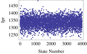
Figure 5.2: Dense random matrices (with $N=4000$). Typical IPR of the initial states.

The IPR in this case is sharply distributed around $N/3$. This finding can be understood through a simple model of random vectors on a N-sphere of unit radius (Porter-Thomas distribution). By a simple integration one finds [30]

$$\langle c_{a}^{4}\rangle\,=\,3/N^{2}\,\,\,,$$ (5.3 )

and therefore the IPR scales as

$$\frac{1}{\sum_{a}c_{a}^{4}}\simeq N/3\,\,\,.$$ (5.4 )

This scaling is confirmed by our data, as shown in Fig. 5.3.

$\begin{array}[]{cc}\includegraphics[width=173.44534pt]{Nonintegrable-dense-meanIpr-scaling-matrix-size.eps}&\includegraphics[width=173.44534pt]{Nonintegrable-dense-maxIpr-scaling-matrix-size.eps}\\ \end{array}$

Figure 5.3: Dense random matrices. IPR vs. matrix size. The red lines are linear fits $y=ax$. Left panel: average IPR on all initial states ($a=0.3336$). Right panel: maximum IPR ($a=0.3764$).

Moreover, the fact that the mean IPR and the maximum IPR almost coincide is confirmation that all initial states are equivalent. This means that the pre-quench and the post-quench bases of the energy eigenvectors are completely random with respect one another. Eigenstates therefore have no reason to be localized in energy.

Let us now turn our attention to the expectation values of observables since the main content of the ETH concerns the distribution of the eigenstate expectation values (EEVs), $\mathcal{O}_{aa}$, and their behavior when the system size is increased. We first report two sample EEV distributions, given in Fig. 5.4, which show no energy dependence.

$\begin{array}[]{cc}\includegraphics[width=173.44534pt]{EEV-sample-even-dense.eps}&\includegraphics[width=173.44534pt]{EEV-sample-odd-dense.eps}\\ \end{array}$

Figure 5.4: Dense random matrices. EEV $\langle E_{a}|{\mathcal{O}}|E_{a}\rangle$ vs $E_{a}$. Left: even observable. Right: odd observable.

We can argue (and we have checked numerically) that the distribution of an intensive observable over the whole energy spectrum shrinks to zero for increasing system size. Moreover, it is not only the variance but even the support of the distribution of the observables that goes to zero inasmuch as the difference of the EEV maximum and minimum is going to zero as $N\rightarrow\infty$ (see Fig. 5.8).

More precisely, we have:

$$\mathcal{O}_{aa}\equiv\langle E_{a}|{\mathcal{O}}|E_{a}\rangle=\sum_{\beta}A_{a,\beta}{\mathcal{O}}_{\beta}\,\,\,,$$ (5.5 )

where $\beta$ indexes the eigenstates, $|\beta\rangle$, of the observable ${\mathcal{O}}$, while ${\mathcal{O}}_{\beta}$ is the corresponding eigenvalue, and $A_{a,\beta}=|\langle E_{a}|\beta\rangle|^{2}$. To estimate the r.h.s. we argue for an equivalency of observables and hold that the IPR of an eigenvector $|E_{a}\rangle$ of the post-quench Hamiltonian relative to the basis of eigenvectors $|\beta\rangle$ equals the IPR of the initial state $|\psi_{0}\rangle$ in the basis $|E_{a}\rangle$. So we can suppose that $\mathcal{O}_{aa}$ can be expanded in terms of a set of $\frac{N}{3}$ states, each of which is given by

$\begin{array}[]{cc}\includegraphics[width=173.44534pt]{EEV-variance-even-dense.eps}&\includegraphics[width=173.44534pt]{EEV-variance-odd-dense.eps}\\ \end{array}$

Figure 5.5: Dense random matrices. EEV variance (averaged over the entire spectrum) vs. matrix size. The continuous line is the fit $a/x^{b}$ with $b=0.9\pm 0.1$. The data points for the even and odd observables exactly overlap in this plot.

$$A_{a,\beta}\simeq\frac{1}{IPR(H\to{\mathcal{O}})}\simeq\frac{3}{N}\,\,\,.$$ (5.6 )

Then, if we assume $A_{a\beta}$ and $A_{a\beta^{\prime}}$ are independent and note that $\mathcal{O}_{aa}$ has zero mean, we obtain

$$\overline{|\mathcal{O}_{aa}|^{2}}\simeq\frac{N}{3}\left(\frac{3\sigma_{\mathcal{O}}}{N}\right)^{2}\simeq\frac{3\sigma_{\mathcal{O}}^{2}}{N},$$

where $\sigma_{\mathcal{O}}^{2}$ is the variance of the spectrum of the observable ${\mathcal{O}}$. In Fig. 5.5, the numerical results are plotted together with a power-law fit and, as expected, the exponent is indeed close to one.

$\begin{array}[]{cc}\includegraphics[width=173.44534pt]{EEV-min-max-even-dense.eps}&\includegraphics[width=173.44534pt]{EEV-min-max-odd-dense.eps}\\ \end{array}$

Figure 5.6: Dense random matrices. Max-min EEV vs. matrix size for the range of even (left) and odd (right) observables (again the behavior of the two is indistinguishable). The continuous line is the fit $a\sqrt{\frac{\ln{N}}{N}}$.

Now let us consider the full support of the distribution of the EEVs where we define $\delta_{\mathcal{O}}$ as the difference of the maximum and the minimum of the EEVs among all the energy eigenstates $|E_{a}\rangle$. Since the distribution is symmetric about zero, we have:

$$\delta_{\mathcal{O}}\,=\,2\max_{a}\{\mathcal{O}_{aa}\}\,.$$ (5.7 )

To estimate the scaling of this quantity, we again approximate all the overlaps $A_{a,\beta}$ as in Eq. (5.6). Therefore we are led to estimate the maximum of the quantity

$${\cal O}_{aa}\equiv\frac{3}{N}\sum_{\beta}^{\prime}{\mathcal{O}}_{\beta},$$

where the prime on the sum indicates that only $1/3$ of the total $\beta$’s are being summed over.

$\begin{array}[]{cc}\includegraphics[width=173.44534pt]{micro-diag_dense-plot-even-center.eps}&\includegraphics[width=173.44534pt]{micro-diag_dense-plot-odd-center.eps}\\ \end{array}$

Figure 5.7: Dense random matrices. $\sigma=\sqrt{({\mathcal{O}}_{\text{micro}}-{\mathcal{O}}_{\text{diag}})^{2}}$ vs. matrix size for initial states laying in the central part of the spectrum $\overline{e}\approx 0$. The continuous line is the fit $a/x^{b}$. Left: even observable $b=1.9\pm 0.1$; right: odd observable $b=2.1\pm 0.1$

As before we suppose that the random variables ${\mathcal{O}}_{\beta}$ are independently distributed according to the intensive semicircle law (${\mathcal{O}}_{\beta}\in[-2,2]$):

$$\rho(x)\equiv\operatorname{Prob}({\mathcal{O}}_{\beta}=x)\,=\,\frac{1}{2\pi}\sqrt{4-x^{2}}\,\,\,.$$ (5.8 )

In this case we can use large deviation theory (see for instance [31]) and it follows that

$$\operatorname{Prob}({\cal O}_{aa}>x)\simeq e^{-NI(x)}\,\,\,,$$ (5.9 )

where $I(x)$ is the rate function given by

$$I(x)=\sup_{\theta}[\theta x-\lambda(\theta)]\,\,\,.$$ (5.10 )

The function $\lambda(x)$ is the cumulant generating function

$$e^{\lambda(\theta)}\,=\,\int_{-2}^{2}\rho(x)e^{x\theta}=\frac{I_{1}(2t)}{t}\,\,\,,$$ (5.11 )

with $I_{1}$ the modified Bessel function of first kind. Now the distribution governing the probability that $\delta_{\cal O}$ is less than a value $M$ is given by

$$\operatorname{Prob}(\delta_{\cal O}<M)=\prod_{a=1}^{N}\operatorname{Prob}({\cal O}_{aa}<M)\simeq\left(1-e^{-NI(M)}\right)^{N}\simeq 1-Ne^{-NI(M)}\,\,\,.$$

We can find the scaling of the typical value of the maximum by requiring that the probability is large enough

$$\operatorname{Prob}(\delta_{\cal O}<M)\simeq\text{const.}\quad\Rightarrow\quad I(M)\simeq\frac{\ln N}{N}\,\,\,.$$

Since $I(x)\xrightarrow{x\to 0}0$, we are interested in the behavior of $I(x)$ for small $x$ and from Eq. (5.10) and Eq. (5.11) we get

$$I(x)\simeq\frac{x^{2}}{2}+O(x^{3})\quad\Rightarrow\quad\delta_{\mathcal{O}}\,\,\,\simeq\sqrt{\frac{\ln N}{N}}\,\,\,.$$ (5.12 )

In Fig. 5.6, one sees the numerical agreement with our heuristic argument.

Finally let’s consider the behaviour of the difference between the diagonal and the microcanonical ensembles with increasing matrix size. To this end, we analyzed the difference $\sigma=\sqrt{({\mathcal{O}}_{\text{micro}}-{\mathcal{O}}_{\text{diag}})^{2}}$ of the two ensembles for each initial state $|\psi_{0}\rangle$. Due to the broad energy distribution of the overlap of the initial states, their intensive energy $\overline{e}=\langle\psi_{0}|H(-h)|\psi_{0}\rangle$ lies in a region, $[-0.5,0.5]$, smaller than the range of the post-quench energies $-2<e_{a}<2$. $\sigma$ show the same behavior independent of the particular initial state $|\psi_{0}\rangle$ being considered, as can be argued by the constant IPR combined with a structureless EEV distribution. As all initial states are equivalent, we focus our attention on those initial states belonging to a small energy window around $e=0$: the result is shown in Fig. 5.7. As can be seen, the difference between micro-canonical and diagonal ensemble rapidly goes to zero as a function of N.

In conclusion, quenches in dense random matrices are characterized by initial states with large IPRs, EEV distributions of the post-quench eigenbasis with no energy dependence and whose variance goes to zero exponentially with increasing system size. In this sense, their thermalization is trivial, as the spread of the micro-diagonal ensemble is governed by a distribution whose support is increasingly localized near zero as system size grows.

6 Thermalization in Sparse Random Matrices

$\begin{array}[]{cc}\includegraphics[width=173.44534pt]{dos-sparse.eps}&\includegraphics[width=173.44534pt]{spacing-sparse.eps}\\ \end{array}$

Figure 6.1: Sparse random matrices (with N=4000). Left: density of states, right: level spacing statistics, the continuous line is the Wigner surmise for GOE matrices.

$\begin{array}[]{cc}\includegraphics[width=173.44534pt]{overlap-sparse-2000thstate-4000.eps}&\includegraphics[width=173.44534pt]{overlap-sparse-3500thstate-4000.eps}\\ \end{array}$

Figure 6.2: Sparse random matrices. Behavior of the overlaps $|c_{a}|^{2}$ for a state midspectrum (left) and for one in the upper portion of the spectrum (right).

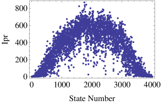
Figure 6.3: Sparse random matrices (with $N=4000$). The IPR for a specific realization. The ordering of the initial states in this plot is according to their energy relative to the post-quench Hamiltonian, $\langle\psi_{0}|H^{>}|\psi_{0}\rangle$.

$\begin{array}[]{cc}\includegraphics[width=173.44534pt]{Nonintegrable-sparse-meanIpr-scaling-matrix-size.eps}&\includegraphics[width=173.44534pt]{Nonintegrable-sparse-maxIpr-scaling-matrix-size.eps}\\ \end{array}$

Figure 6.4: Sparse random matrices. IPR vs. matrix size. The continuous line is the $y=ax$ fit. Left, average IPR on the whole spectrum ($a=0.0738$). Right, maximum IPR ($a=0.2096$).

We now turn to the more interesting case of thermalization in sparse random matrices. As we have indicated such matrices describe the Hamiltonians of systems with local interactions. In order to define the ensemble of these matrices, we employed a symmetric mask matrix, $\mathcal{M}$. This matrix has $1$’s on the diagonal and in each of its rows we allow it to have on average $\ln N$ off-diagonal entries equal to $1$. All remaining entries of the mask matrix are equal to zero. See Appendix B for details of how $\mathcal{M}$ is defined. The upper triangular part of the (symmetric) Hamiltonian is then obtained as:

$$H(h)_{i<j}=\left\{\begin{array}[]{ll}d_{i}\leavevmode\nobreak\ {\rm with\leavevmode\nobreak\ }d_{i}{\rm\leavevmode\nobreak\ drawn\leavevmode\nobreak\ from\leavevmode\nobreak\ }\mathcal{N}(0,\ln N)&{\rm if}\leavevmode\nobreak\ i=j;\\ o_{ij}\times\mathcal{M}_{ij}\leavevmode\nobreak\ {\rm with\leavevmode\nobreak\ }o_{ij}{\rm\leavevmode\nobreak\ drawn\leavevmode\nobreak\ from\leavevmode\nobreak\ }\mathcal{N}(0,1)&{\rm if}\leavevmode\nobreak\ i<j,\end{array}\right.$$ (6.1 )

where $\mathcal{N}(\mu,\sigma^{2})$ is a normal distribution with $\mu$ mean and $\sigma^{2}$ variance. Then the coefficients in the off-diagonal blocks are multiplied times $h$ to reproduce the structure in Eq. (4.1). The different choice for the variances of the diagonal $d_{i}$ and off-diagonal elements $o_{ij}$ is motivated by the requirement that the spectrum be extensive.

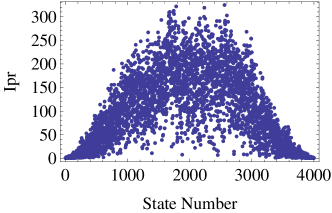
Figure 6.5: Sparse random matrices (with $N=4000$). The IPR of the post-quench eigenstates w.r.t. the local basis for a specific realization. The ordering of the initial states in this plot is according to their energy eigenvalue.

$\begin{array}[]{cc}\includegraphics[width=173.44534pt]{Nonintegrable-sparse-meanIpr-scaling-matrix-size-wrt-localbasis-c0.0314.eps}&\includegraphics[width=173.44534pt]{Nonintegrable-sparse-maxIpr-scaling-matrix-size-matrix-size-wrt-localbasis-c0.162.eps}\\ \end{array}$

Figure 6.6: Sparse random matrices. IPR w.r.t. local basis vs. matrix size. The continuous line is the $y=ax$ fit. Left, average IPR on the whole spectrum ($a=0.0321$). Right, maximum IPR ($a=0.1632$).

In fact we can compute the variance of the spectrum:

$$\sigma_{H}^{2}\equiv\frac{\operatorname{Tr}(H^{2})}{N}\simeq 2\ln N.$$ (6.2 )

In the approximation in which the eigenvalues $E_{a}$ are considered independent and normally distributed, one can relate the minimum of the spectrum with the variance, obtaining for the groundstate energy the estimate

$$E_{\text{gs}}=\min_{a}\{E_{a}\}\simeq-\sigma_{H}\sqrt{2\ln N}\simeq-2\ln N.$$

The eigenvalues midspectrum will be at most a few standard deviations $\sigma_{H}$ from the average $0$. Thus a typical eigenstate will be such that

$$E_{a}^{(0)}-E_{\text{gs}}^{(0)}\propto\ln{N}\,\,\,.$$ (6.3 )

We see then that our choices satisfy the requirement that energy is an extensive quantity.

We compare these estimates with numerics in Fig. 6.1 where we plot the density of states and the level spacing distribution for one realization of a sparse matrix. The density of states is no longer a semicircle, looking rather more like a bell-shaped distribution. Moreover, notice that, unlike the GOE case where the intensive quantities have a finite distribution in the large $N$ limit, i.e.Eq. (5.8), in this sparse case the (intensive) standard deviation behaves as $\frac{1}{\sqrt{\ln N}}$, while the support of the spectrum remains approximately $[-2,2]$. We also see from the right side of Fig. 6.1 that the level-spacing distribution obeys the Wigner form for a non-integrable model.

To generate the observables we follow a similar procedure, i.e. we employ the same mask $\mathcal{M}$. The idea behind this choice is that the matrix $\mathcal{M}$ is responsible for the local structure in the Hilbert space and so we keep it for all the physical observables (including the Hamiltonian itself). So we have for the upper triangular part of a symmetric observable

$$\mathcal{O}_{i<j}=\left\{\begin{array}[]{ll}d_{i}{\rm\leavevmode\nobreak\ with\leavevmode\nobreak\ }d_{i}{\rm\leavevmode\nobreak\ drawn\leavevmode\nobreak\ from\leavevmode\nobreak\ }\mathcal{N}(0,1/\ln N)&i=j;\\ o_{ij}\times M_{ij}{\rm\leavevmode\nobreak\ with\leavevmode\nobreak\ }o_{ij}{\rm\leavevmode\nobreak\ drawn\leavevmode\nobreak\ from\leavevmode\nobreak\ }\mathcal{N}(0,1/(\ln N)^{2})&i\neq j.\end{array}\right.$$

The even and odd parts are then obtained as before by splitting $\mathcal{O}$ into diagonal and off-diagonal blocks.

$\begin{array}[]{cc}\includegraphics[width=173.44534pt]{EEV-sample-even-sparse.eps}&\includegraphics[width=173.44534pt]{EEV-sample-odd-sparse.eps}\\ \end{array}$

Figure 6.7: Sparse random matrices. EEV $\langle E_{a}|{\mathcal{O}}|E_{a}\rangle$ vs $e_{a}$. Left: even observable. Right: odd observable

6.1 Numerical results

Unlike the dense case, in sparse random matrices the overlap distributions are peaked around the initial state post-quench intensive energy $\overline{e}$, as can be seen in two examples shown in Fig. 6.2.

The IPR is no longer constant (as it was for the random dense matrices), but shows behaviour dependent on the energy of the initial state, as demonstrated in Fig. 6.3. However there is still scaling of the IPR with the matrix size, as can be seen by studying the behaviour of the maximum IPR vs the matrix size, plotted in Fig. 6.4. In this case the mean and the maximum IPR are rather different, due to the presence of states with very small IPR.

We see a similar phenomena when we study the IPR of the pre-quench and post-quench (they are statistically equivalent) eigenbasis relative to the local basis (that is, the basis of states in which the Hamiltonian matrices, $H(h^{<})$ and $H(h^{>})$ are expressed). We see in Fig.6.6 that the mean and max IPR’s here as a function of matrix size, $N$, are similar to those in Fig. 6.4.

$\begin{array}[]{cc}\includegraphics[width=173.44534pt]{EEV-variance-even-sparse-fullspectrum.eps}&\includegraphics[width=173.44534pt]{EEV-variance-odd-sparse-fullspectrum.eps}\\ \end{array}$

Figure 6.8: Sparse random matrices. EEV variance vs. matrix size for the full spectrum. The continuous lines are the fit $a/x^{b}$. Left: even observable $b=0.50\pm 0.01$ Right: odd observable $b=0.75\pm 0.01$.

$\begin{array}[]{cc}\includegraphics[width=173.44534pt]{EEV-min-max-even-sparse-fullspectrum.eps}&\includegraphics[width=173.44534pt]{EEV-min-max-odd-sparse-fullspectrum.eps}\\ \end{array}$

Figure 6.9: Sparse random matrices. Max-min EEV vs matrix size for the full spectrum. Left: even observable. Right: odd observable.

The equivalency of these two different IPRs is not surprising. If we pick an eigenstate of the pre-quench Hamiltonian, $|\psi_{0}\rangle$, that has a small IPR relative to the local basis, it will necessarily be only weakly coupled to the off-diagonal blocks, particularly as the Hamiltonian matrices are sparse. $|\psi_{0}\rangle$ will then be closely related to some post-quench eigenstate. This implies in turn that $|\psi_{0}\rangle$ will have a small IPR relative to the post-quench eigenbasis. Similarly a pre-quench eigenstate $|\psi_{0}\rangle$ with a large IPR in terms of the local basis will be strongly affected by the quench in the sense that it is unrelated to any eigenstate of the post-quench eigenbasis, and so will have a large IPR in terms of this basis. It is this that lies behind the similar shapes of Fig. 6.5 and Fig. 6.3.

The behavior of the IPR relative to the local basis (and, by this equivalency, the IPR relative to the post-quench eigenbasis) can be understood directly in the framework of Anderson localization [37]. Even though our problem is a many body one, our sparse Hamiltonian can be seen as akin to the dynamics of a non-interacting particle hopping on a Bethe-lattice of fixed connectivity, $\ln N$, where each site has a random potential (the diagonal part of the random Hamiltonian). It is well known [36] that for this model the Anderson localization transition occurs with the presence of a mobility edge which separates the delocalized states (in the middle of the band) from the localized states (in the tails of the energy spectrum). In our case localization occurs when the $IPR$ is $O(1)$, while delocalization is seen for $IPR=O(N)$.

$\begin{array}[]{cc}\includegraphics[width=173.44534pt]{EEV-variance-even-sparse-center.eps}&\includegraphics[width=173.44534pt]{EEV-variance-odd-sparse-center.eps}\\ \end{array}$

Figure 6.10: Sparse random matrices. EEV variance vs. matrix size for a small energy window around $e=0$. The continuous line is the fit $a/x^{b}$. Left: even observable $b=1.29\pm 0.01$. Right: odd observable $b=1.2\pm 0.1$.

$\begin{array}[]{cc}\includegraphics[width=173.44534pt]{EEV-min-max-even-sparse-center.eps}&\includegraphics[width=173.44534pt]{EEV-min-max-odd-sparse-center.eps}\\ \end{array}$

Figure 6.11: Sparse random matrices. Max-min EEV vs. matrix size for a small energy window around $e=0$ in logscale. The continuous line is the fit $a/x^{b}+c$. Left: even observable $e=0$, $b=0.65\pm 0.01$, $c=0.067\pm 0.001$. Right: odd observable $e=0$, $b=0.50\pm 0.01$, $c=0.01\pm 0.01$.

$\begin{array}[]{cc}\includegraphics[width=173.44534pt]{EEV-min-max-even-sparse-e1.eps}&\includegraphics[width=173.44534pt]{EEV-min-max-odd-sparse-e1.eps}\\ \end{array}$

Figure 6.12: Sparse random matrices. Max-min EEV vs. matrix size for a small energy window around $e=1$. The continuous line is the fit $a/x^{b}+c$. Left: even observable $e=1$, $b=0.35\pm 0.01$, $c=1.7\pm 0.1$. Right: odd observable $e=1$, $b=0.33\pm 0.01$, $c=0.14\pm 0.01$.

The position, $E_{m}$, of the mobility edge can be determined by the following equation, derived along the same lines as [36]

$$2\ln N\int_{0}^{\infty}\{p^{\prime}(x-E_{m})-p^{\prime}(E_{m}-x)\}\ln x\,dx=1\,\,\,,$$ (6.4 )

where $p(x)$ is the probability density of the diagonal terms in our Hamiltonian

$$p(x)=\frac{1}{\sqrt{2\pi\ln N}}\exp\left(-\frac{x^{2}}{2\ln N}\right)\,\,\,.$$ (6.5 )

States with an $|E|>|E_{m}|$ such that the right hand side of Eq. (6.4) is less than $1$ are localized. Otherwise they are delocalized. The integral in Eq. (6.4) can be estimated at the leading order in the large $N$ limit, and one obtains

$$1=\exp\left(-\frac{E_{m}^{2}}{2\ln N}\right)\ln\ln N\sqrt{\frac{2\ln N}{\pi}}\quad\Rightarrow\quad E_{m}\simeq\pm\sqrt{\ln N\ln\ln N}\,\,\,.$$ (6.6 )

Thus in the large $N$ limit all the states with a non-zero intensive energy $E/\ln N$ behave as localized. Nonetheless the majority of the states, as they are concentrated in a window of width $\sigma_{H}$ (given in Eq. 6.2) and as $E_{m}/\sigma_{H}\gg 1$, will be delocalized with an $IPR=O(N)$.

$\begin{array}[]{cc}\includegraphics[width=173.44534pt]{micro-diag_sparse-plot-even-center.eps}&\includegraphics[width=173.44534pt]{micro-diag_sparse-plot-odd-center.eps}\\ \end{array}$

Figure 6.13: Sparse random matrices. $\sigma=\sqrt{({\mathcal{O}}_{\text{micro}}-{\mathcal{O}}_{\text{diag}})^{2}}$ vs. matrix size for initial states laying in the central part of the spectrum $\overline{e}\approx 0$. The continuous lines are the fits $a/x^{b}$. Left: even observable $b=1.15\pm 0.01$. Right: odd observable $b=1.30\pm 0.01$.

$\begin{array}[]{cc}\includegraphics[width=173.44534pt]{micro-diag_sparse-plot-even-e1.eps}&\includegraphics[width=173.44534pt]{micro-diag_sparse-plot-odd-e1.eps}\\ \end{array}$

Figure 6.14: Sparse random matrices. $\sigma=\sqrt{({\mathcal{O}}_{\text{micro}}-{\mathcal{O}}_{\text{diag}})^{2}}$ vs. matrix size for initial states laying in a small window around $e=1$. The continuous lines are the fits $a/x^{b}$. Left: even observable $b=0.31\pm 0.01$. Right: odd observable $b=0.44\pm 0.01$.

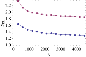
Figure 6.15: Sparse random matrices. Kullback-Leibler entropy vs matrix size for the center of the spectrum for the uniform (squares) and the Gaussian distribution (circles).

The localization of states with finite intensive energies has implications for the EEV distribution vs. $e_{a}$. As the observables have a matrix structure closely related to that of the Hamiltonians, we expect that localized states to be close to eigenstates of the observables itself, in contrast with Eq. (5.6) in the dense case. On such states, the observables will have expectation values far from their zero average. On the contrary, the delocalized states midspectrum will have EEV values closer to the mean of zero. In Fig. 6.7 we see numerical verification of this.

This result marks a strong difference with respect to the case of dense matrices. We also see marked differences between the sparse and dense cases with both the variance and the support of the EEVs distribution of the observable, as shown in Fig. 6.8 and 6.9: while the variance approaches zero as $N$ grows, the support does not, instead tending to a non-zero constant. Therefore the scaling Eq. (5.12) is no longer applicable, most likely as the overlaps, $A_{i\beta}$, and the eigenvalues of the observable, $O_{\beta}$, in Eq. (5.5) can no longer be considered as independent.

Since the distribution of the overlap coefficients, $c_{a}$, are peaked around the energy $\overline{e}=\langle\psi_{0}|H(h)|\psi_{0}\rangle$, it is worthwhile to analyze the scaling behavior of the distribution of the EEVs in the vicinity of a specific $\bar{e}$. Here we choose two different energy windows, one centered around $\bar{e}=0$, lying exactly mid-spectrum and one around $\bar{e}=1$. For $\bar{e}=0$ the variance and the max-min spread as functions of the size $N$ are plotted in Fig. (6.10) and Fig. (6.11). It is this distribution that is going to determine whether with respect to a particular observable we see thermalization. We again see that the variance is going to zero, while in contrast to the full spectrum, the max-min spread seems to tend, asymptotically, to either a very small constant value or to zero. The errors in our numerics are then not small enough to tell us at $\bar{e}=0$ whether there is a complete absence of rare states. However we can be more definitive for the energy window centered at $\bar{e}=1$. In this window we see (as evidenced in Fig. 6.12) that the max-min spread of the EEV’s in the large N limit tends to a finite constant for both the even and odd observables.

Our numerical data then suggests that there are rare states where the observable remains far from its average value in each microcanonical energy window corresponding to non-zero intensive energy, differently for what has been observed in the $t-J$ model [33, 34, 35]. In these studies of the t-J model, rare states were argued to be absent for a range of strengths of the next nearest neighbour interaction, $V^{\prime}$, and for an energy window centered mid-spectrum. In particular with $V^{\prime}$ small the t-J model is effectively integrable and rare states were found to be present and with $V^{\prime}$ large, the model develops energy bands, also compatible with the existence of rare states. It is for a middle range of $V^{\prime}$ that rare states were then found to be absent. Our own study sees some agreement with these results. And it is natural to think there would be some agreement at least. Our study of random matrix model should correspond to the $t-J$ model with intermediate values of $V^{\prime}$: our matrix models are neither integrable nor do they have any notion of energy bands. In our case, rare states (at least for what we call the odd observable) seem to be vanishing as system size increases exactly in the center of the spectrum. However away from this midpoint of the spectrum, we find that rare states do exist, even in the thermodynamic limit. It would thus be interesting to extend the work of [33, 34, 35] to additional energy windows.

Following [32], we then conclude in the case of sparse matrices that thermalization may depend on the particular nature of the initial state and will not occur when such rare states are given a proportionally large weight in the decomposition of the initial state. We, however, do not find for the particular initial conditions specified by our quench protocol that the rare states are given disproportional weight such that thermalization does not occur. For both energy windows $\bar{e}=0$ (see Fig. (6.13)) and $\bar{e}=1$ (Fig. (6.14)), we see that with increasing matrix size the difference between the diagonal and microcanonical ensembles averaged over all initial conditions tends to zero. This implies that the weighting of rare states in our initial states is not preponderant. We do note however that the vanishing of the difference between ensembles decreases considerably more slowly with system size for the energy window, $\bar{e}=1$, than for $\bar{e}=0$. We might ascribe this to the presence of rare states at this energy – even though these states do not lead to non-thermalization in the thermodynamic limit, they may slow the approach to a thermalized state as the system size is increased.

We verify this by computing the Kullback-Leibler entropy. This entropy is an information theoretic tool used to estimate how close two distributions are. It is defined as

$$S_{KL}=\sum_{a}P(a)\ln{\frac{P(a)}{Q(a)}}\,\,\,,$$ (6.7 )

where $P(a)$ is the expected distribution and $Q(a)$ is the distribution to be compared. $S_{KL}$ is zero if the two distributions coincide except for sets of zero measures. In our case we choose $P(a)=|c_{a}|^{2}$ and $Q(a)$ to belong to either a uniform or a Gaussian distribution centered about the energy $\overline{e}$. The range over which $Q(a)$ is defined has been taken such that the variances of $Q$ and $P$ coincides. Fig. 6.15 shows the average KL-entropy vs. matrix size for the central part of the spectrum which indicates in both cases a slow decay as the system size is increased. The slow approach of the distribution $P(a)$ to a distribution $Q(a)$ that is both smooth and symmetric about $\bar{e}$ suggests that rare states are not weighted in a peculiar way, thus permitting thermalization.

In conclusion, for sparse random matrices our numerical data is compatible with the existence of rare states. However, the initial states selected by the quench protocol do not seem to have large overlaps with these rare states and so we typically find thermalization as the end result of our quench process.

7 Time Scales of Thermalization

$\begin{array}[]{cc}\includegraphics[width=173.44534pt]{timeEvol.eps}&\includegraphics[width=173.44534pt]{fluctEvol.eps}\\ \end{array}$

Figure 7.1: Left: time evolution of the observable $\mathcal{O}_{t}$ versus time $t$. Right: time evolution of the fluctuations $\Delta_{t}^{\mathcal{O}}/\Delta_{0}^{\mathcal{O}}$ versus time $t$, logscale on $y$ axis. The straight line is the exponential fit whose slope defines $\tau_{S}$.

The sparse random ensemble, inasmuch as it mimics some characteristic properties of thermalization in systems with local Hamiltonians, is the right framework to address the study of the thermalization time. Interest in this quantity can be traced back to the seminal paper by Von Neumann [6] regarding the quantum ergodic theorem (QET). The statement made in von Neumann’s paper is that, under suitable assumptions (the Hamiltonian has no resonances - meaning that the energy level differences are non degenerate), any state $|\psi_{0}\rangle$ in the energy shell $[e-\Delta,e+\Delta]$, will thermalize for most choices of the observable and most times $t$, i.e.

$$\mathcal{O}_{t}\,=\,\langle\psi_{0}(t)|\mathcal{O}|\psi_{0}(t)\rangle=\operatorname{Tr}(\mathcal{O}\rho_{\text{mc}})\qquad\text{for almost all }t,\mathcal{O}\,\,\,.$$

To make the notion of (macroscopic) observable and “most” used here precise would require the development of an involved technical apparatus and so instead we refer the reader to the existing literature [6, 7]. Nonetheless we can say there are important differences between this quantum thermalization and the classical notion of ergodicity where a time-average is involved. It is therefore of interest to give a precise estimate of the time needed for thermalization. There have been different approaches which have tried to clarify this question [39, 40, 41, 42]. In Fig. 7.1, we examine the typical behavior of a realization of a random observable, $\mathcal{O}_{t}$. It decays towards the average value given by the diagonal ensemble:

$$\mathcal{O}_{\infty}=\operatorname{Tr}(\mathcal{O}\rho_{\text{diag}})\,\,\,,$$

and we define the time $\tau_{F}$ as the first time at which $\mathcal{O}_{t}$ meets $\mathcal{O}_{\infty}$.

$\begin{array}[]{cc}\includegraphics[width=173.44534pt]{timeScalingSlow.eps}&\includegraphics[width=173.44534pt]{timeScalingFast.eps}\\ \end{array}$

Figure 7.2: Scaling with the matrix size of the two time scale $\tau_{S}$ (left) with a linear fit ($-3.94+0.066N$) and $\tau_{F}$ (right) with a logarithmic fit ($-28.61+8.60\ln N$).

We stress here, that even if this quantity has not a direct physical interpretation, it can be considered as a lower bound for the thermalization time. The time evolution of the observable however keeps fluctuating around the average, due to finite system size, with it coming close to its initial value after a time, $\tau_{rec}$, the recurrence time. To quantify these fluctuations we define

$$\Delta^{\mathcal{O}}_{t}\equiv\frac{1}{t}\int_{0}^{t}(\mathcal{O}_{t}-\mathcal{O}_{\infty})^{2}d\tau\xrightarrow{t\to\infty}\sum_{a,b}c_{a}^{2}c_{b}^{2}O_{ab}^{2}\equiv\Delta^{\mathcal{O}}_{\infty}\,\,\,,$$

where we have assumed the absence of energy degeneracies and resonances. The quantity $\Delta^{\mathcal{O}}_{t}$ can be considered as the variance in the time interval $[0,t]$ of the observable and its behavior is plotted in Fig. 7.1: relaxation to the infinite time value is found as expected. We can fit this curve supposing an exponential relaxation, $e^{-t/\tau_{S}}$, defining in this way another time scale, $\tau_{S}$, the time interval needed for the relaxation of the fluctuations. Notice that this quantity is the one closer to the Von Neumann formulation: indeed, from the Chebyshev inequality, one has a bound on the fraction, $\mu/t$, of times where the observable has an expectation value far from its average

$$\frac{\mu(\tau\in[0,t]\;{\rm\leavevmode\nobreak\ and\leavevmode\nobreak\ }\;|{\cal O}_{\tau}-\mathcal{O}_{\infty}|>a)}{t}<\frac{\Delta^{\mathcal{O}}_{t}}{a^{2}}\,\,\,.$$

As in the thermodynamic limit $\Delta^{\mathcal{O}}_{\infty}\to 0$, this fraction must also go to zero in the long time limit. In Fig. 7.2, we see the comparison between the two timescales $\tau_{S}$ and $\tau_{F}$ versus the system size. From this plot one can see clearly that $\tau_{S}$ is a long time-scale, with a behavior proportional to $N$, i.e. the size of the Hilbert space. Notice that this can also be interpreted as the minimum spectral gap and at the leading order in $N$:

$$\min_{a\neq b}|E_{a}-E_{b}|\propto\frac{1}{N}.$$

In contrast, $\tau_{F}$ is characterized by a much slower scaling with the size of the system and is therefore a fast time-scale. Although it is not easy to extract the precise scaling law from the available data, we have fit this data with the form

$$\tau_{F}(N)=a\ln N\,\,\,,$$

and so taking the scaling of this time scale to go as the volume. In contrast, the time scale for dense matrices was recently argued to go as the inverse of the volume[41].

8 Conclusions

In this paper we have addressed the issues of thermalization and the Eigenstate Thermalization Hypothesis in the framework of random matrices, aiming to identify certain statistical properties of quantum extended systems subjected to a quench process. For this purpose we focused our attention on $Z_{2}$ breaking quantum Hamiltonians, among the simplest theoretical quench protocols. In an attempt to encode in our analysis the property of locality, we have considered the ensemble of sparse random matrices and we have compared the data coming from this ensemble with similar data extracted from the ensemble of dense random matrices. We have found reliable evidence of different behavior in the two ensembles. These differences show up both in the IPR of the quench states and in the distribution of the expectation values of the observables on post-quench energy eigenstates. In particular, while in the dense random matrix ensemble both the variance and the support of the observables vanish with increasing system size $L$, the sparse random matrix ensemble sees instead strong indications that the variance of EEVs goes to zero while the support remains finite as $L\rightarrow\infty$. The different behavior of the two ensembles can be traced back to the different density of states exhibited by the two sets of matrices: while in the dense matrices all states are delocalized in the Hilbert space, with almost equal overlap on all energy eigenstates, in the sparse matrices there are instead both delocalized and localized states. Localized states give rise to rare values of the expectation values of the observables, i.e. values which differ from the typical ones sampled by the micro-canonical ensemble. If properly weighted, such localized states may give rise to a breaking of thermalization. In the absence of such weighting, as seems to be the case in the initial conditions chosen by our quench protocol, one instead observes relaxation to the thermal value of the local observables.

In the framework of sparse random matrices, we have also provided numerical estimates of the different time scales of thermalization. We have found that it is possible to identify two time scales: a fast one $\tau_{F}$ and a slow one $\tau_{S}$, and that they depend differently upon the size of the system.

Acknowledge

We are grateful to M. Rigol, L. Santos, P. Calabrese, V. Kravtsov and M. Müeller for useful discussions. RMK acknowledges support by the US DOE under contract number DE-AC02-98 CH 10886.

Appendix A Total momentum and quasiparticles

We want to consider in this appendix the effect of a change of basis on the sparseness of the Hamiltonian matrix. In particular we will focus on a change to a basis where momentum is a good quantum number. We take once again the Ising case as a guiding example. Changing the basis, the new matrix representation of the Hamiltonian Eq. (2.1) can be obtained in terms of an unitary matrix $U$:

$$\mathcal{H}^{\prime}\,=\,U^{\dagger}\,\mathcal{H}\,U$$ (1.1 )

and, for a general change of basis, the resulting matrix will not be sparse anymore; this is quite intuitive: for an arbitrary unitary matrix $U$, i.e. an arbitrary basis, any notion of locality is lost.

However we can ask what happens in a much more common case: is the Hamiltonian still sparse in the basis of momenta? We will show that there is a subtle issue related to the definition of this change of basis. To be more specific, let’s put the Ising Hamiltonian on a circle by introducing periodic boundary conditions such that the $(L+1)$-th site is identified with the first one. In this case the system becomes translationally invariant; this can be formally written as:

$$[H,T]=0,$$

where $T$ is the shift operator, defined by:

$$T|m_{1},\ldots,m_{L}\rangle=|m_{L},m_{1},\ldots,m_{L-1}\rangle.$$

Clearly we have:

$$T^{L}=\mathbf{1},$$ (1.2 )

and therefore we can define the total momentum $P$ as:

$$T=e^{iP}\Rightarrow[H,P]=0.$$

As $T$ is a unitary operator, using Eq. (1.2) we easily deduce the usual structure of the spectrum of $P$ as $\frac{2\pi n}{L}$. The basis of momenta is then the basis of the eigenstates of the total momentum. However, the eigenvalues of $P$ are highly degenerate and so many definitions are possible. Two examples will demonstrate that sparseness depends on which definition is employed.

Let us first construct a complete set of eigenstates of $P$ in the following way. We first pick a state $|s\rangle=|m_{1},\ldots m_{L}\rangle$ in the real-space basis. We obtain an invariant subspace for $T$ by considering the set of states:

$$I_{s}=\operatorname{Span}\{|s\rangle,T|s\rangle,T^{2}|s\rangle,\ldots,T^{L_{s}-1}|s\rangle\}$$

where $L_{s}$ is been defined as:

$$L_{s}\equiv\min\{n{\rm\leavevmode\nobreak\ such\leavevmode\nobreak\ that\leavevmode\nobreak\ }T^{n}|s\rangle=|s\rangle\}$$

The eigenstates of $P$ composed of linear combination of states in the set $I_{s}$ can be written as:

$$|\tilde{s}_{n}\rangle=\sum_{k=0}^{L_{s}-1}e^{\frac{2\pi ink}{L_{s}}}T^{k}|s\rangle\quad\Rightarrow\quad P|\tilde{s}_{n}\rangle=\frac{2\pi n}{L_{s}}|\tilde{s}_{n}\rangle.$$ (1.3 )

A full basis of eigenstates for $P$ can be obtained repeating this procedure for different states $|s\rangle$: we call this basis the rigid-translation Fourier basis (RTFB). It is easy to understand that the resulting matrix in this new basis is still sparse. In fact each state is a superposition of at most $L$ states and it follows the corresponding transformation $U$ contains at most $L$ non-zero entries in each row and column. Using Eq. (1.1), we conclude that the Hamiltonian matrix in this basis is still sparse having at most $L^{3}$ non-zero entries in each row ($L^{3}\ll 2^{L}$).

Is this the end of the story? Let us consider what happens if we use a different momentum basis. To this end we work in a second-quantization framework and focus upon a set of operators satisfying (where the $\pm$ stands for the fermionic and bosonic case):

$$[a_{i},a^{\dagger}_{j}]_{\pm}=\delta_{ij}.$$

These operators create and destroy a single particle excitation at position $i$. A real-space basis can be written in this formalism as:

$$(a^{\dagger}_{1})^{n_{1}}(a^{\dagger}_{2})^{n_{2}}\ldots|\Omega\rangle.$$ (1.4 )

The same formalism can be adopted in the Ising case by setting: $a^{\dagger}_{i}\simeq S^{+}_{i}$ and taking $|\Omega\rangle\equiv|\downarrow\ldots\downarrow\rangle$. Here we can define an excitation with defined momentum by setting:

$$\mathfrak{a}^{\dagger}_{k}=\sum_{j=0}^{L-1}e^{ikj}a_{j}^{\dagger}.$$

Putting the inverse of this expression into Eq. (1.4), we get a new basis of eigenstates of total momentum $P$:

$$P\mathfrak{a}^{\dagger}_{k_{1}}\mathfrak{a}^{\dagger}_{k_{2}}\ldots|\Omega\rangle=\left(\sum_{i}k_{i}\right)\mathfrak{a}^{\dagger}_{k_{1}}\mathfrak{a}^{\dagger}_{k_{2}}\ldots|\Omega\rangle.$$ (1.5 )

We call this the single-particle Fourier basis (SPFB). However once we restrict to a subspace where $P$ is defined (appearing as a block for the Hamiltonian matrix), there is a strong difference between this case and the one defined in Eq. (1.4): in fact here, not only the full state but each component excitation has a defined momentum. To better understand this difference we consider a two particle case (in the one particle case, there are no differences between the two momentum bases). Consider a state $|s\rangle=S^{\dagger}_{x_{1}}S^{\dagger}_{x_{2}}|\Omega\rangle=|x_{1},x_{2}\rangle$, that is the state with only two up spins in positions, $x_{1}$ and $x_{2}$. In the RTFB, this state can be expressed as a linear combination of $L$ states, $|\tilde{s}_{n}\rangle$, with $n=0,\ldots,L-1$, where $|\tilde{s}_{n}\rangle$ are obtained as superpositions of the rigid translations, $T^{k}|s\rangle$. In these translated states the distance $|x_{2}-x_{1}|$ between up states always remains the same. On the other hand, with the SPFB, each two-particle state has a non-zero matrix element with $|x_{1},x_{2}\rangle$:

$$\langle x_{1},x_{2}|\mathfrak{a}_{k_{1}}^{\dagger}\mathfrak{a}_{k_{2}}^{\dagger}|\Omega\rangle=\sum_{j_{1},j_{2}}e^{i(k_{1}j_{1}+k_{2}j_{2})}\langle x_{1},x_{2}|j_{1},j_{2}\rangle=e^{i(k_{1}x_{1}+k_{1}x_{2})}+e^{i(k_{1}x_{2}+k_{1}x_{1})}.$$

Increasing the number of particles to $M$, in the RTFB case we always have one summation with $\simeq L$ terms. Instead in the SPFB, we will have $M$ summations, corresponding to $\simeq L^{M}$ terms.

The conclusions we can draw from these considerations are that:

• A local Hamiltonian will appear as a sparse matrix in the real-space basis.

• If we consider the Fourier basis obtained as a superposition of the rigid translations of the real-space basis, the Hamiltonian will appear again as a sparse matrix though perhaps with a larger density of non-zero entries. This is true simply because the change of basis we are considering is sparse.

• If we consider the Fourier basis obtained taking the Fourier transform of single particle states, the change of basis in each block of defined total momentum will not be sparse. In the general case, the Hamiltonian matrix will be characterized by dense blocks of fixed total momentum.

Appendix B Generation of the mask

Our aim is to generate a mask, telling us where the non-zero entries are, according to the scaling Eq. (2.4). The most obvious choice would be simply to take the mask such that each non-diagonal entry is chosen independently, being one with probability $\rho=\frac{\ln N}{N}$ and zero otherwise: $\rho_{0}=1-\rho$. But a simple computation shows that with this choice the probability $P_{nc}$ of having a column (or row) with all the non-diagonal entries equal to zero will be quite high

$$P_{nc}\simeq 1-\left(1-\rho_{0}^{N}\right)^{N}\xrightarrow{N\to\infty}\frac{e-1}{e}\simeq 63\%.$$

To avoid this, we try to fix the number of non-zero entries in each row. However, since at the end, we will need a symmetric matrix with one on the diagonal, we follow a slightly more complicated procedure. We first generate “half” of the mask matrix and at the end we symmetrize by summing it with its transpose. To be more precise, for each row, $i$, of the matrix we generate a set, $R_{i}$, composed of integers drawn from the set $\{1,\ldots,\hat{i},\ldots,N\}$, i.e. a set where the element $i$ is missing. The size, $n_{i}$, of $R_{i}$ has probability $P_{in}$ of equaling $n$ where we define $P_{in}$ by

$$P_{in}=\{q\}\delta_{n-1,\lfloor q\rfloor}+(1-\{q\})\delta_{n,\lfloor q\rfloor}$$

where $\{q\}$ and $\lfloor q\rfloor$ represent respectively the fractional and integer part of $q$ and $q$ is defined by:

$$q=(N-1)-\sqrt{(N-1)^{2}-(N-1)\ln N}.$$

In this way, the size of the $R_{i}$’s will be either $\lfloor q\rfloor$ or $\lfloor q\rfloor+1$, but such that the average is $\bar{n}_{i}=q$. The sets $R_{i}$’s contain the indexes of the non-zero elements in each row. We now define the mask joining each row with the corresponding column, thus symmetrizing the matrix:

$$\mathcal{M}_{ij}=\left\{\begin{array}[]{ll}1&(i=j)\vee(j\in R_{i})\vee(i\in R_{j});\\ 0&\text{otherwise}.\end{array}\right.$$

Our choice of $q$ takes into account the possibility of elements overlapping between the row and the corresponding column, ensuring we have the correct number of non-zero elements in each row:

$$\overline{\#\{j\;|\;\mathcal{M}_{ij}\neq 0\}}=1+2q-\frac{q^{2}}{N-1}=1+\ln N.$$

Notice that the number of non-zero elements in each row is not fixed, because small fluctuations are induced by the symmetrization procedure; however we can be sure that it will be greater than $\lfloor q\rfloor$. We recall that $\ln N/N$ is exactly the threshold for the connectedness of the Erdos-Renyi graph [38]: with this procedure there will be no isolated subblocks, as is confirmed by the Wigner-Dyson level statistics shown in Fig. 6.1.

References

- [1] T. Kinoshita, T. Wenger, D.S. Weiss, Nature 440, 900 903 (2006).
- [2] S. Hofferberth, I. Lesanovsky, B. Fischer, T. Schumm, J. Schmiedmayer, Nature 449, 324 (2007).
- [3] C.N. Weiler, T. W. Neely, D. R. Sherer, A. S. Bradley, M. J. Davis, and B. P. Anderson, Nature, 455, 948 (2008).
- [4] M. Greiner, O. Mandel, T. Esslinger, T. W. Hänsch, and I. Bloch, Nature, 415, 39 (2002).
- [5] L.E. Sadler, J. M. Higbie, S. R. Leslie, M. Vengalattore, and D. M. Stamper-Kurn, Nature, 443, 312 (2006).
- [6] J. von Neumann, Ann. Math. 32 (1931), 191.
- [7] S. Goldstein, J.L. Lebowitz, R. Tumulka, N. Zanghi, European Physical Journal H: Historical Perspectives on Contemporary Physics, 35, 173 (2010).
- [8] J.M. Deutsch, Phys. Rev. A 43 (1991), 2046.
- [9] M. Srednicki, Phys. Rev. E 50 (1994), 888. M. Srednicki, J. Phys. A: Math. Gen. 32 (1999), 1163.
- [10] M. Berry, J. Phys. A 10, 2083 (1977).
- [11] M. Rigol, V. Dunjko and M. Olshanii, Nature 452 (2008), 854
- [12] E. Barouch, B. M. McCoy, and M. Dresden, Phys. Rev. A 2, 1075 (1970); E. Barouch and B. M. McCoy, Phys. Rev. A 3, 2137 (1971).
- [13] K. Sengupta, S. Powell, and S. Sachdev, Phys. Rev. A 69, 053616 (2004).
- [14] D. Rossini, A. Silva, G. Mussardo, and G.E. Santoro, Phys. Rev. Lett. 102, 127204 (2009); D. Rossini, S. Suzuki, G. Mussardo, G.E. Santoro, and A. Silva, Phys. Rev. B 82, 144302 (2010).
- [15] P. Calabrese, F.H.L. Essler, M Fagotti, Phys. Rev. Lett. 106, 227203 (2011).
- [16] J. Mossel, J.S. Caux, New J. Phys. 12 055028 (2010).
- [17] E. Canovi, D. Rossini, R. Fazio, G. E. Santoro, and A. Silva, Phys. Rev. B 83, 094431 (2011).
- [18] C. De Grandi, V. Gritsev, A. Polkovnikov, Phys. Rev. B 81, 012303 (2010).
- [19] P. Calabrese and J. Cardy, Phys. Rev. Lett. 96, 136801 (2006); J. Stat. Mech.: Theory Exp. (2007) P06008.
- [20] M.A. Cazalilla, Phys. Rev. Lett. 97, 156403 (2006); A. Iucci, M.A. Cazalilla, Phys. Rev. A 80, 063619 (2009); A. Iucci, M.A. Cazalilla, Phys. Rev. A 80, 063619 (2009).
- [21] A. Mitra and T. Giamarchi, Phys. Rev. B 85, 075117 (2012).
- [22] M. Rigol, V. Dunjko, V. Yurovsky, and M. Olshanii, Phys. Rev. Lett. 98, 050405 (2007); M. Rigol, A. Muramatsu, and M. Olshanii, Phys. Rev. A 74, 053616 (2006).
- [23] D. Fioretto, G. Mussardo, New J. Phys. 12 055015 (2010).
- [24] M. Rigol, V. Dunjko, and M. Olshanii, Nature 452, 854 (2008)
- [25] M. Rigol, Phys. Rev. Lett. 103, 100403 (2009); Phys. Rev. A 80, 053607 (2009).
- [26] C. Kollath, A. M. Läuchli, and E. Altman, Phys. Rev. Lett. 98, 180601 (2007).
- [27] S. R. Manmana, S. Wessel, R. M. Noack, and A. Muramatsu, Phys. Rev. Lett. 98, 210405 (2007).
- [28] M. Eckstein, M. Kollar, and P. Werner, Phys. Rev. Lett. 103, 056403 (2009); M. Eckstein and M. Kollar, Phys. Rev. Lett. 100, 120404 (2008); M. Kollar and M. Eckstein, Phys. Rev. A 78, 013626 (2008).
- [29] M.L. Mehta, Random Matrices, Academic Press, New York 1991.
- [30] F. Haake, Quantum Signatures of Chaos, Springer, Berlin, 2nd edn., (2001). 479
- [31] R.S. Ellis, Entropy, Large Deviations and Statistical Mechanics, Springer Publication. ISBN 3-540-29059-1.
- [32] G. Biroli, C. Kollath and A.M. Läuchli, Phys. Rev. Lett. 105 (2010), 250401.
- [33] L. F. Santos and M. Rigol, Phys. Rev. E 81, 036206 (2010).
- [34] M. Rigol and L. F. Santos, Phys. Rev. A 82, 011604(R) (2010).
- [35] L. F. Santos and M. Rigol, Phys. Rev. E 82, 031130 (2010).
- [36] R. Abou-Chacra, P.W. Anderson and D.J. Thouless, J. Phys. C: Solid State Phys. 6 (1973) 1734
- [37] P.W. Anderson, Phys. Rev. 109 (1958) 1492-1505
- [38] P. Erdös and A. Rényi Publicationes Mathematicae 6: 290–297. (1959)
- [39] Vinayak and M. Žnidarič, arXiv:1107.6035 (2011)
- [40] L. Masanes, A.J. Roncaglia, and A. Acin, arXiv: 1108.0374 (2011)
- [41] F. G. S. L. Brandão, P. Ćwikliński, M. Horodecki, P. Horodecki, J. Korbicz, and M. Mozrzymas, arXiv: 1108.2985 (2011)
- [42] A. J. Short and T. C. Farrelly, arXiv: 1110.5759 (2011)