CFTP/11-019
Seesaw neutrino masses from an $A_{4}$ model
with two equal vacuum expectation values

Abstract

We present a model for the lepton sector, with $A_{4}$ horizontal-symmetry group, in which two of the Higgs doublets in an $A_{4}$ triplet of Higgs doublets have equal vacuum expectation values. The model makes well-defined predictions for the effective light-neutrino Majorana mass matrix. We show that those predictions are compatible with the experimental data.

1 Introduction

Particle physics now boasts an impressive knowledge of the three light-neutrino masses, $m_{1,2,3}$, and of lepton mixing. The latter is parametrized by the mixing matrix

$$U=\left(\begin{array}[]{ccc}c_{12}c_{13}&s_{12}c_{13}&s_{13}e^{-i\delta}\\ -s_{12}c_{23}-c_{12}s_{23}s_{13}e^{i\delta}&c_{12}c_{23}-s_{12}s_{23}s_{13}e^{i\delta}&s_{23}c_{13}\\ s_{12}s_{23}-c_{12}c_{23}s_{13}e^{i\delta}&-c_{12}s_{23}-s_{12}c_{23}s_{13}e^{i\delta}&c_{23}c_{13}\end{array}\right),$$ (1)

where $c_{m}=\cos{\theta_{m}}$ and $s_{m}=\sin{\theta_{m}}$ for $m\in\left\{12,13,23\right\}$. That knowledge is summarized in table 1,

parameter	best-fit value	$3\sigma$ interval
$m_{2}^{2}-m_{1}^{2}$ (in $10^{-5}~{}\mathrm{eV}^{2}$)	7.59	[7.09, 8.19]
$\left|m_{3}^{2}-m_{1}^{2}\right|$ (in $10^{-3}~{}\mathrm{eV}^{2}$)	$\begin{array}[]{c}2.50\\[-5.69054pt] 2.40\end{array}$	$\begin{array}[]{c}[2.14,2.76]\\[-2.84526pt] [2.13,2.67]\end{array}$
$s_{12}^{2}$	0.312	[0.27, 0.36]
$s_{23}^{2}$	0.52	[0.39, 0.64]
$s_{13}^{2}$	$\begin{array}[]{c}0.013\\[-5.69054pt] 0.016\end{array}$	$\begin{array}[]{c}[0.001,0.035]\\[-2.84526pt] [0.001,0.039]\end{array}$

Table 1: Experimental data for the neutrino masses and for lepton mixing. In the cases of $\left|m_{3}^{2}-m_{1}^{2}\right|$ and of $s_{13}^{2}$, the upper (lower) line corresponds to the case of a normal (inverted) neutrino mass spectrum.

which is borrowed in abridged form from reference [1]. Notice that we do not know the absolute mass scale of the neutrinos. We also ignore whether the neutrino mass spectrum is ‘normal’, i.e. with $m_{3}>m_{1,2}$, or ‘inverted’, i.e. with $m_{3}<m_{1,2}$. Finally, we lack much information on the phase $\delta$, which remains essentially free.

Flavour physics would like to find a rationale for these experimental data by imposing ‘horizontal’ symmetries on the leptonic Lagrangian and by assuming a pattern of (spontaneous or soft) breaking of those symmetries. A review of some achievements in this field can be found in reference [3]. In particular, a horizontal-symmetry group much used in this context has been $A_{4}$ [4], which is the smallest group with a triplet irreducible representation. Models using $A_{4}$ [5] usually feature a horizontal-$A_{4}$ triplet of scalar ‘Higgs’ gauge-$SU(2)$ doublets; in that triplet either only one Higgs doublet has nonzero vacuum expectation value (VEV) or all three Higgs doublets have equal VEVs.

This paper presents a new model using horizontal-symmetry group $A_{4}$ in the lepton sector. The model has the novel feature that in the $A_{4}$ triplet of Higgs doublets two of the doublets have equal VEVs (different from the VEV of the third doublet). Subsection 2.3 explains how such a vacuum can come about.

The model that we suggest uses the type-I seesaw mechanism and makes clear-cut predictions. Let the symbol $M$ denote the effective Majorana (hence symmetric) light-neutrino mass matrix in the basis where the charged-lepton mass matrix is diagonal. Then those predictions are

$$M_{ee}M_{\mu\mu}M_{\tau\tau} = M_{e\mu}M_{e\tau}M_{\mu\tau},$$ (2)

$$M_{\mu\mu}\left(M_{e\tau}\right)^{2} = M_{\tau\tau}\left(M_{e\mu}\right)^{2}.$$ (3)

These predictions are invariant under a rephasing of $M$, i.e. under the transformation

$$M_{\alpha\alpha^{\prime}}\to e^{i\left(\psi_{\alpha}+\psi_{\alpha^{\prime}}\right)}M_{\alpha\alpha^{\prime}},$$ (4)

for $\alpha,\alpha^{\prime}\in\left\{e,\mu,\tau\right\}$. They thus embody four real constraints on $M$, just as when $M$ has either two vanishing matrix elements [6] or two vanishing minors [7].

In section 2 we present our model. In section 3 we display its predictions by means of scatter plots for the various observables. A brief summary of our achievements is given in section 4.

2 The model

2.1 Fields and symmetries

We envisage an extension of the Standard Model, with gauge group $SU(2)\times U(1)$, in which there are three right-handed neutrinos $\nu_{1,2,3R}$ and four scalar $SU(2)$ doublets $\Phi_{1,2,3,4}$. As usual, there are three left-handed lepton $SU(2)$ doublets $D_{\alpha L}$ and three right-handed charged-lepton $SU(2)$ singlets $\alpha_{R}$. The quark sector will not be dealt with in this paper, but the model can in principle be extended to accomodate it.

The model has horizontal-symmetry group $A_{4}$. The group $A_{4}$ is generated by two transformations, $S$ and $T$. Those transformations act in the following way:

$$S:\quad\nu_{2R}\to-\nu_{2R},\ \nu_{3R}\to-\nu_{3R},\ \Phi_{2}\to-\Phi_{2},\ \Phi_{3}\to-\Phi_{3};$$ (5)

$$T: \nu_{1R}\to\nu_{2R}\to\nu_{3R}\to\nu_{1R},\ \Phi_{1}\to\Phi_{2}\to\Phi_{3}\to\Phi_{1},$$ (6)

$$D_{\mu L}\to\omega D_{\mu L},\ D_{\tau L}\to\omega^{2}D_{\tau L},\ \mu_{R}\to\omega\mu_{R},\ \tau_{R}\to\omega^{2}\tau_{R},$$

where $\omega=\exp\left(2i\pi/3\right)$. The Higgs doublet $\Phi_{4}$ and the lepton multiplets $D_{eL}$ and $e_{R}$ are $A_{4}$-invariant.

2.2 Lagrangian

Let $\Phi_{j}=\left(\begin{array}[]{c}\phi_{j}^{+}\\ \phi_{j}^{0}\end{array}\right)$ ($j\in\left\{1,2,3,4\right\}$) and let $v_{j}$ denote the VEV of $\phi_{j}^{0}$. The masses of the charged leptons originate in Yukawa couplings to $\Phi_{4}$:

$$\mathcal{L}_{\ell\mathrm{Yukawa}}=-\left(\sum_{\alpha=e,\mu,\tau}\frac{m_{\alpha}}{v_{4}}\bar{D}_{\alpha L}\alpha_{R}\right)\Phi_{4}+\mathrm{H.c.};$$ (7)

we may choose the phase of $\alpha_{R}$ in such a way that $m_{\alpha}$ is real and positive. The charged-lepton mass matrix is automatically diagonal because of the horizontal symmetry.

The Majorana mass terms of the right-handed neutrinos are

$$\mathcal{L}_{\mathrm{Maj}}=m\sum_{k=1}^{3}\nu_{kR}^{T}C^{-1}\nu_{kR}+\mathrm{H.c.},$$ (8)

where $C$ is the charge-conjugation matrix in Dirac space. Because of the horizontal symmetry, $\mathcal{L}_{\mathrm{Maj}}$ is proportional to the unit matrix in flavour space. Therefore, the effective light-neutrino Majorana mass matrix following from the type-I seesaw mechanism is simply

$$M=-\frac{1}{m}M_{D}M_{D}^{T},$$ (9)

where $M_{D}$ is the Dirac mass matrix connecting the left-handed to the right-handed neutrinos.

The Yukawa couplings of the right-handed neutrinos are given by

$$\mathcal{L}_{\nu\mathrm{Yukawa}} = a\bar{D}_{eL}\left(\nu_{1R}\tilde{\Phi}_{1}+\nu_{2R}\tilde{\Phi}_{2}+\nu_{3R}\tilde{\Phi}_{3}\right)$$ (10)

$$+b\bar{D}_{\mu L}\left(\nu_{1R}\tilde{\Phi}_{1}+\omega^{2}\nu_{2R}\tilde{\Phi}_{2}+\omega\nu_{3R}\tilde{\Phi}_{3}\right)$$

$$+c\bar{D}_{\tau L}\left(\nu_{1R}\tilde{\Phi}_{1}+\omega\nu_{2R}\tilde{\Phi}_{2}+\omega^{2}\nu_{3R}\tilde{\Phi}_{3}\right)+\mathrm{H.c.},$$

where $\tilde{\Phi}_{j}\equiv\left(\begin{array}[]{cc}0&1\\ -1&0\end{array}\right)\Phi_{j}^{\ast}=\left(\begin{array}[]{c}{\phi_{j}^{0}}^{\ast}\\ -\phi_{j}^{-}\end{array}\right)$ and $a$, $b$, and $c$ are complex dimensionless coupling constants. It follows from equation (10) that

$$M_{D}=\left(\begin{array}[]{ccc}av_{1}^{\ast}&av_{2}^{\ast}&av_{3}^{\ast}\\ bv_{1}^{\ast}&\omega^{2}bv_{2}^{\ast}&\omega bv_{3}^{\ast}\\ cv_{1}^{\ast}&\omega cv_{2}^{\ast}&\omega^{2}cv_{3}^{\ast}\end{array}\right).$$ (11)

The scalar potential is

$$V = \mu_{1}\left(\Phi_{1}^{\dagger}\Phi_{1}+\Phi_{2}^{\dagger}\Phi_{2}+\Phi_{3}^{\dagger}\Phi_{3}\right)+\mu_{2}\,\Phi_{4}^{\dagger}\Phi_{4}$$ (12)

$$+\lambda_{1}\left[\left(\Phi_{1}^{\dagger}\Phi_{1}\right)^{2}+\left(\Phi_{2}^{\dagger}\Phi_{2}\right)^{2}+\left(\Phi_{3}^{\dagger}\Phi_{3}\right)^{2}\right]+\lambda_{2}\left(\Phi_{4}^{\dagger}\Phi_{4}\right)^{2}$$

$$+\lambda_{3}\left(\Phi_{1}^{\dagger}\Phi_{1}\,\Phi_{2}^{\dagger}\Phi_{2}+\Phi_{1}^{\dagger}\Phi_{1}\,\Phi_{3}^{\dagger}\Phi_{3}+\Phi_{2}^{\dagger}\Phi_{2}\,\Phi_{3}^{\dagger}\Phi_{3}\right)$$

$$+\lambda_{4}\,\Phi_{4}^{\dagger}\Phi_{4}\left(\Phi_{1}^{\dagger}\Phi_{1}+\Phi_{2}^{\dagger}\Phi_{2}+\Phi_{3}^{\dagger}\Phi_{3}\right)$$

$$+\lambda_{5}\left(\left|\Phi_{1}^{\dagger}\Phi_{2}\right|^{2}+\left|\Phi_{1}^{\dagger}\Phi_{3}\right|^{2}+\left|\Phi_{2}^{\dagger}\Phi_{3}\right|^{2}\right)$$

$$+\lambda_{6}\left(\left|\Phi_{1}^{\dagger}\Phi_{4}\right|^{2}+\left|\Phi_{2}^{\dagger}\Phi_{4}\right|^{2}+\left|\Phi_{3}^{\dagger}\Phi_{4}\right|^{2}\right)$$

$$+\left\{\lambda_{7}e^{i\zeta_{7}}\left[\left(\Phi_{1}^{\dagger}\Phi_{2}\right)^{2}+\left(\Phi_{2}^{\dagger}\Phi_{3}\right)^{2}+\left(\Phi_{3}^{\dagger}\Phi_{1}\right)^{2}\right]\right.$$

$$+\lambda_{8}e^{i\zeta_{8}}\left[\left(\Phi_{1}^{\dagger}\Phi_{4}\right)^{2}+\left(\Phi_{2}^{\dagger}\Phi_{4}\right)^{2}+\left(\Phi_{3}^{\dagger}\Phi_{4}\right)^{2}\right]$$

$$+\lambda_{9}e^{i\zeta_{9}}\left(\Phi_{2}^{\dagger}\Phi_{3}\,\Phi_{1}^{\dagger}+\Phi_{3}^{\dagger}\Phi_{1}\,\Phi_{2}^{\dagger}+\Phi_{1}^{\dagger}\Phi_{2}\,\Phi_{3}^{\dagger}\right)\Phi_{4}$$

$$\left.+\lambda_{10}e^{i\zeta_{10}}\left(\Phi_{3}^{\dagger}\Phi_{2}\,\Phi_{1}^{\dagger}+\Phi_{1}^{\dagger}\Phi_{3}\,\Phi_{2}^{\dagger}+\Phi_{2}^{\dagger}\Phi_{1}\,\Phi_{3}^{\dagger}\right)\Phi_{4}+{\rm H.c.}\right\},$$

where $\lambda_{1\mbox{--}10}$ are real.

2.3 Vacuum

In its particle content and symmetries, hence in its Lagrangian, the present model is almost identical to the one of Hirsch et al. [8]. The two models differ, though, in the assumed form of the vacuum state.

We write the VEVs as

$$\left\langle 0\left|\phi_{j}^{0}\right|0\right\rangle\equiv v_{j}=\sqrt{V_{j}}\,e^{i\vartheta_{j}},$$ (13)

where the $\sqrt{V_{j}}$ are real and positive by definition. Without loss of generality we set $\vartheta_{4}=0$. We furthermore define

$$\chi_{1} = \vartheta_{1}-\vartheta_{2}-\vartheta_{3},$$ (14)

$$\chi_{2} = \vartheta_{2}-\vartheta_{3}-\vartheta_{1},$$ (15)

$$\chi_{3} = \vartheta_{3}-\vartheta_{1}-\vartheta_{2}.$$ (16)

Then, the vacuum potential is given by

$$\mathcal{V} = \mu\left(V_{1}+V_{2}+V_{3}\right)+\lambda_{1}\left(V_{1}^{2}+V_{2}^{2}+V_{3}^{2}\right)$$ (17)

$$+\left(\lambda_{3}+\lambda_{5}\right)\left(V_{1}V_{2}+V_{1}V_{3}+V_{2}V_{3}\right)$$

$$+2\lambda_{7}\left[V_{1}V_{2}\cos{\left(\zeta_{7}+\chi_{2}-\chi_{1}\right)}+V_{2}V_{3}\cos{\left(\zeta_{7}+\chi_{3}-\chi_{2}\right)}\right.$$

$$\left.+V_{3}V_{1}\cos{\left(\zeta_{7}+\chi_{1}-\chi_{3}\right)}\right]$$

$$+2\lambda_{8}V_{4}\left[V_{1}\cos{\left(\zeta_{8}+\chi_{2}+\chi_{3}\right)}+V_{2}\cos{\left(\zeta_{8}+\chi_{3}+\chi_{1}\right)}\right.$$

$$\left.+V_{3}\cos{\left(\zeta_{8}+\chi_{1}+\chi_{2}\right)}\right]$$

$$+2\sqrt{V_{1}V_{2}V_{3}V_{4}}\left\{\lambda_{9}\left[\cos{\left(\zeta_{9}+\chi_{1}\right)}+\cos{\left(\zeta_{9}+\chi_{2}\right)}+\cos{\left(\zeta_{9}+\chi_{3}\right)}\right]\right.$$

$$\left.+\lambda_{10}\left[\cos{\left(\zeta_{10}+\chi_{1}\right)}+\cos{\left(\zeta_{10}+\chi_{2}\right)}+\cos{\left(\zeta_{10}+\chi_{3}\right)}\right]\right\},$$

where

$$\mathcal{V} = \left\langle 0\left|V\right|0\right\rangle-\mu_{2}V_{4}-\lambda_{2}V_{4}^{2},$$ (18)

$$\mu = \mu_{1}+\left(\lambda_{4}+\lambda_{6}\right)V_{4}.$$ (19)

The equations for vacuum stationarity are

$$0=\frac{\partial\mathcal{V}}{\partial V_{1}} = \mu+2\lambda_{1}V_{1}+\left(\lambda_{3}+\lambda_{5}\right)\left(V_{2}+V_{3}\right)$$ (20)

$$+2\lambda_{7}\left[V_{2}\cos{\left(\zeta_{7}+\chi_{2}-\chi_{1}\right)}+V_{3}\cos{\left(\zeta_{7}+\chi_{1}-\chi_{3}\right)}\right]$$

$$+2\lambda_{8}V_{4}\cos{\left(\zeta_{8}+\chi_{2}+\chi_{3}\right)}$$

$$+\sqrt{\frac{V_{2}V_{3}V_{4}}{V_{1}}}\left\{\lambda_{9}\left[\cos{\left(\zeta_{9}+\chi_{1}\right)}+\cos{\left(\zeta_{9}+\chi_{2}\right)}+\cos{\left(\zeta_{9}+\chi_{3}\right)}\right]\right.$$

$$\left.+\lambda_{10}\left[\cos{\left(\zeta_{10}+\chi_{1}\right)}+\cos{\left(\zeta_{10}+\chi_{2}\right)}+\cos{\left(\zeta_{10}+\chi_{3}\right)}\right]\right\},$$

$$0=\frac{\partial\mathcal{V}}{\partial V_{2}} = \mu+2\lambda_{1}V_{2}+\left(\lambda_{3}+\lambda_{5}\right)\left(V_{1}+V_{3}\right)$$ (21)

$$+2\lambda_{7}\left[V_{3}\cos{\left(\zeta_{7}+\chi_{3}-\chi_{2}\right)}+V_{1}\cos{\left(\zeta_{7}+\chi_{2}-\chi_{1}\right)}\right]$$

$$+2\lambda_{8}V_{4}\cos{\left(\zeta_{8}+\chi_{3}+\chi_{1}\right)}$$

$$+\sqrt{\frac{V_{1}V_{3}V_{4}}{V_{2}}}\left\{\lambda_{9}\left[\cos{\left(\zeta_{9}+\chi_{1}\right)}+\cos{\left(\zeta_{9}+\chi_{2}\right)}+\cos{\left(\zeta_{9}+\chi_{3}\right)}\right]\right.$$

$$\left.+\lambda_{10}\left[\cos{\left(\zeta_{10}+\chi_{1}\right)}+\cos{\left(\zeta_{10}+\chi_{2}\right)}+\cos{\left(\zeta_{10}+\chi_{3}\right)}\right]\right\},$$

$$0=\frac{\partial\mathcal{V}}{\partial V_{3}} = \mu+2\lambda_{1}V_{3}+\left(\lambda_{3}+\lambda_{5}\right)\left(V_{1}+V_{2}\right)$$ (22)

$$+2\lambda_{7}\left[V_{1}\cos{\left(\zeta_{7}+\chi_{1}-\chi_{3}\right)}+V_{2}\cos{\left(\zeta_{7}+\chi_{3}-\chi_{2}\right)}\right]$$

$$+2\lambda_{8}V_{4}\cos{\left(\zeta_{8}+\chi_{1}+\chi_{2}\right)}$$

$$+\sqrt{\frac{V_{1}V_{2}V_{4}}{V_{3}}}\left\{\lambda_{9}\left[\cos{\left(\zeta_{9}+\chi_{1}\right)}+\cos{\left(\zeta_{9}+\chi_{2}\right)}+\cos{\left(\zeta_{9}+\chi_{3}\right)}\right]\right.$$

$$\left.+\lambda_{10}\left[\cos{\left(\zeta_{10}+\chi_{1}\right)}+\cos{\left(\zeta_{10}+\chi_{2}\right)}+\cos{\left(\zeta_{10}+\chi_{3}\right)}\right]\right\},$$

$$0=\frac{\partial\mathcal{V}}{\partial\chi_{1}} = 2\lambda_{7}V_{1}\left[V_{2}\sin{\left(\zeta_{7}+\chi_{2}-\chi_{1}\right)}-V_{3}\sin{\left(\zeta_{7}+\chi_{1}-\chi_{3}\right)}\right]$$ (23)

$$-2\lambda_{8}V_{4}\left[V_{2}\sin{\left(\zeta_{8}+\chi_{3}+\chi_{1}\right)}+V_{3}\sin{\left(\zeta_{8}+\chi_{1}+\chi_{2}\right)}\right]$$

$$-2\sqrt{V_{1}V_{2}V_{3}V_{4}}\left[\lambda_{9}\sin{\left(\zeta_{9}+\chi_{1}\right)}+\lambda_{10}\sin{\left(\zeta_{10}+\chi_{1}\right)}\right],$$

$$0=\frac{\partial\mathcal{V}}{\partial\chi_{2}} = 2\lambda_{7}V_{2}\left[V_{3}\sin{\left(\zeta_{7}+\chi_{3}-\chi_{2}\right)}-V_{1}\sin{\left(\zeta_{7}+\chi_{2}-\chi_{1}\right)}\right]$$ (24)

$$-2\lambda_{8}V_{4}\left[V_{3}\sin{\left(\zeta_{8}+\chi_{1}+\chi_{2}\right)}+V_{1}\sin{\left(\zeta_{8}+\chi_{2}+\chi_{3}\right)}\right]$$

$$-2\sqrt{V_{1}V_{2}V_{3}V_{4}}\left[\lambda_{9}\sin{\left(\zeta_{9}+\chi_{2}\right)}+\lambda_{10}\sin{\left(\zeta_{10}+\chi_{2}\right)}\right],$$

$$0=\frac{\partial\mathcal{V}}{\partial\chi_{3}} = 2\lambda_{7}V_{3}\left[V_{1}\sin{\left(\zeta_{7}+\chi_{1}-\chi_{3}\right)}-V_{2}\sin{\left(\zeta_{7}+\chi_{3}-\chi_{2}\right)}\right]$$ (25)

$$-2\lambda_{8}V_{4}\left[V_{1}\sin{\left(\zeta_{8}+\chi_{2}+\chi_{3}\right)}+V_{2}\sin{\left(\zeta_{8}+\chi_{3}+\chi_{1}\right)}\right]$$

$$-2\sqrt{V_{1}V_{2}V_{3}V_{4}}\left[\lambda_{9}\sin{\left(\zeta_{9}+\chi_{3}\right)}+\lambda_{10}\sin{\left(\zeta_{10}+\chi_{3}\right)}\right].$$

(The stationarity equation of $\left\langle 0\left|V\right|0\right\rangle$ relative to variations of $V_{4}$ will be written down later.) It is clear that solutions to equations (20)–(25) with $v_{2}=v_{3}$, i.e. with $V_{2}=V_{3}$ and $\chi_{2}=\chi_{3}$, exist if and only if $\zeta_{7}=0$ or $\pi$, cf. equations (21) and (22), (24) and (25). From now on we assume that a symmetry CP is present at the Lagrangian level, which enforces $\zeta_{7}=\zeta_{8}=\zeta_{9}=\zeta_{10}=0$ (remember that $\lambda_{7\mbox{--}10}$ are real and may be either positive or negative). We may then assume that the vacuum has $v_{2}=v_{3}$, with

$$0 = \mu+2\lambda_{1}V_{1}+2\left(\lambda_{3}+\lambda_{5}\right)V_{2}+4\lambda_{7}V_{2}\cos{\left(\chi_{2}-\chi_{1}\right)}$$ (26)

$$+2\lambda_{8}V_{4}\cos{\left(2\chi_{2}\right)}+\lambda_{s}V_{2}\sqrt{\frac{V_{4}}{V_{1}}}\left(\cos{\chi_{1}}+2\cos{\chi_{2}}\right),$$

$$0 = \mu+2\lambda_{1}V_{2}+\left(\lambda_{3}+\lambda_{5}\right)\left(V_{1}+V_{2}\right)+2\lambda_{7}\left[V_{2}+V_{1}\cos{\left(\chi_{2}-\chi_{1}\right)}\right]$$ (27)

$$+2\lambda_{8}V_{4}\cos{\left(\chi_{1}+\chi_{2}\right)}+\lambda_{s}\sqrt{V_{1}V_{4}}\left(\cos{\chi_{1}}+2\cos{\chi_{2}}\right),$$

$$0 = 2\lambda_{7}V_{1}\sin{\left(\chi_{2}-\chi_{1}\right)}-2\lambda_{8}V_{4}\sin{\left(\chi_{1}+\chi_{2}\right)}-\lambda_{s}\sqrt{V_{1}V_{4}}\sin{\chi_{1}},$$ (28)

$$0 = \lambda_{7}V_{1}V_{2}\sin{\left(\chi_{1}-\chi_{2}\right)}-\lambda_{8}V_{4}\left[V_{2}\sin{\left(\chi_{1}+\chi_{2}\right)}+V_{1}\sin{\left(2\chi_{2}\right)}\right]$$ (29)

$$-\lambda_{s}V_{2}\sqrt{V_{1}V_{4}}\sin{\chi_{2}},$$

where $\lambda_{s}=\lambda_{9}+\lambda_{10}$.

In order to get a feeling for what is at stake, let us consider CP-conserving solutions to equations (26)–(29) with $\chi_{1}=\chi_{2}=0$. (In our actual fits we shall always use spontaneously CP-breaking solutions; this paragraph should be understood merely as an illustration of the consequences of $\lambda_{s}\neq 0$.) Then, equations (28) and (29) are automatically satisfied while equations (26) and (27) read

$$2\lambda_{1}V_{1}+2\lambda_{m}V_{2}+3\lambda_{s}V_{2}\sqrt{\frac{V_{4}}{V_{1}}} = -\bar{\mu},$$ (30)

$$2\lambda_{1}V_{2}+\lambda_{m}\left(V_{1}+V_{2}\right)+3\lambda_{s}\sqrt{V_{1}V_{4}} = -\bar{\mu},$$ (31)

where

$$\lambda_{m} = \lambda_{3}+\lambda_{5}+2\lambda_{7},$$ (32)

$$\bar{\mu} = \mu+2\lambda_{8}V_{4}.$$ (33)

There is a solution to equations (30) and (31) with $V_{1}=V_{2}$. If and only if $\lambda_{s}\neq 0$, there is also a solution with (in general) $V_{1}\neq V_{2}$,

$$\sqrt{V_{4}} = \frac{2\lambda_{1}-\lambda_{m}}{3\lambda_{s}}\sqrt{V_{1}},$$ (34)

$$V_{2} = \frac{-\bar{\mu}-2\lambda_{1}V_{1}}{2\lambda_{1}+\lambda_{m}}.$$ (35)

Note that $\lambda_{s}\neq 0$ is crucial for the existence of this solution. The presence in the potential of the terms with coefficients $\lambda_{9}$ and $\lambda_{10}$ leads to the existence of stationarity points with $V_{2}=V_{3}\neq V_{1}$.

2.4 The neutrino mass matrix

We assume that the stationarity point of the scalar potential found in the previous subsection, with $v_{2}=v_{3}$, is indeed the global minimum of the potential, i.e. we assume that the vacuum state has

$$v_{2}=v_{3}.$$ (36)

Then, according to equations (9) and (11),

$$M=-\frac{1}{m}\left(\begin{array}[]{ccc}a^{2}r&abs&acs\\ abs&b^{2}s&bcr\\ acs&bcr&c^{2}s\end{array}\right).$$ (37)

where

$$r = {v_{1}^{\ast}}^{2}+2{v_{2}^{\ast}}^{2},$$ (38)

$$s = {v_{1}^{\ast}}^{2}-{v_{2}^{\ast}}^{2}$$ (39)

are in general complex and have unrelated phases. The Yukawa couplings $a$, $b$, and $c$ must be taken real in equation (37), since we have assumed CP symmetry at the Lagrangian level.

The light-neutrino mass matrix in equation (37) obeys the two rephasing-invariant constraints in equations (2) and (3). Another remarkable feature of the matrix in equation (37) is that it preserves its form when it is inverted, i.e. $M^{-1}$ is of the same form as $M$ and also satisfies the constraints (2) and (3).

3 Fits

In the basis where the charged-lepton mass matrix is diagonal, the neutrino Majorana mass matrix $M$ is bi-diagonalized by the lepton mixing matrix $U$:

$$M=U^{\ast}DU^{\dagger},$$ (40)

where

$$D=\mathrm{diag}\left(m_{1},\,m_{2}e^{-i\chi_{21}},\,m_{3}e^{-i\chi_{31}}\right).$$ (41)

In our numerical work we have inputted random initial values of the neutrino masses, of the phases $\chi_{21}$ and $\chi_{31}$, and of the parameters of $U$, within their respective $3\sigma$ intervals given in table 1 (parameters which are not in that table were taken free). We computed the matrix $M$ by using equation (40). We have then step-by-step adjusted the input parameters in order to eventually fit the constraints (2) and (3).

For each of the fits thus obtained, we have calculated

$$\frac{r}{s}=\frac{M_{ee}M_{\mu\mu}}{\left(M_{e\mu}\right)^{2}}$$ (42)

and therefrom obtained

$$\frac{v_{2}}{v_{1}}=\sqrt{\frac{r^{\ast}-s^{\ast}}{r^{\ast}+2s^{\ast}}}=\sqrt{\frac{V_{2}}{V_{1}}}\,\exp{\left(i\ \frac{\chi_{2}-\chi_{1}}{2}\right)}.$$ (43)

We have further inputted random values of $V_{1}$, $V_{4}$, $\chi_{1}$, and of the parameters $\lambda_{1,2,3,4,6,7,9}$. By using the four stationarity equations (26)–(29) together with

$$0=\frac{\partial\left\langle 0\left|V\right|0\right\rangle}{\partial V_{4}} = \mu_{2}+2\lambda_{2}V_{4}+\left(\lambda_{4}+\lambda_{6}\right)\left(V_{1}+2V_{2}\right)$$ (44)

$$+2\lambda_{8}\left[V_{1}\cos{\left(2\chi_{2}\right)}+2V_{2}\cos{\left(\chi_{1}+\chi_{2}\right)}\right]$$

$$+\lambda_{s}\sqrt{\frac{V_{1}}{V_{4}}}\,V_{2}\left(\cos{\chi_{1}}+2\cos{\chi_{2}}\right),$$

we have calculated the remaining five parameters of the potential, i.e. $\lambda_{5,8,10}$ and $\mu_{1,2}$. We have then computed the neutral and charged-scalar mass matrices at this stationarity point and discarded the point whenever any of the physical scalars displayed a negative squared mass, i.e. we have made sure that the stationarity point is indeed a local minimum of the potential. We have also checked that the correct number of Goldstone bosons is present at each local minimum.

We have discovered that many of the local minima of the potential thus found display low-mass scalars; indeed, all the local minima feature at least one low-mass physical neutral scalar. In order to contain this problem of low-mass scalars, we have discarded any minima in which either a charged scalar or more than one neutral scalar has mass smaller than $100~{}\mathrm{GeV}$. The masses were normalized through

$$V_{1}+2V_{2}+V_{4}=\left(174~{}\mathrm{GeV}\right)^{2}.$$ (45)

In this way we have constructed two sets of points, of approximately 1,800 points each, one of them with normal and the other one with inverted neutrino mass spectra, obeying the constraints (2) and (3) and which are local minima of the scalar potential with all the physical scalars but one having a high mass. These are the points that we next display in various scatter plots. In all figures but for figures 1 and 2, blue (red) points are those with a normal (inverted) neutrino mass spectrum.

We first focus on the predictions of our model for the absolute neutrino mass scale. In figures 1 and 2 we display histograms of the lowest neutrino mass for our sets of points. One sees that the neutrino masses tend to be lower when the mass spectrum is normal; points with an inverted spectrum sometimes display neutrino masses which are almost degenerate, with $m_{3}\sim\sqrt{m_{1}^{2}-m_{3}^{2}}\approx 0.05~{}\mathrm{eV}$. In contrast, points with a normal neutrino mass spectrum usually display a markedly hierarchical spectrum, i.e. one with $m_{1}\ll\sqrt{m_{3}^{2}-m_{1}^{2}}$.

In figure 3 the phase $\delta$ is plotted against the mass term $\left|M_{ee}\right|$; the latter is the quantity relevant for neutrinoless double-$\beta$ decay. One sees once again that points with an inverted spectrum display higher masses—$\left|M_{ee}\right|$ is there typically $0.02~{}\mathrm{eV}$ but it is much lower for points with normal neutrino spectra. In our model there is no prediction for $\delta$ in the case of a normal spectrum, while $\left|\sin{\delta}\right|\ \mbox{\raisebox{-3.0pt}{$\stackrel{{\scriptstyle\displaystyle<}}{{\sim}}$}}\ 0.5$ when the neutrino mass spectrum is inverted.

Figure 4 gives the prediction of our model for the reactor mixing angle $\theta_{13}$. Notice that, in our search for fits, we have enforced the condition that all the observables be within their respective $3\sigma$ intervals displayed in the third column of table 1; this explains the blank areas in the lower part and in both sides of figure 4. One sees in that figure that our model predicts a very small $\theta_{13}$—$\sin^{2}{\theta_{13}}$ is always smaller than one half the current best-fit values. Since the experimental indications for a non-zero $\theta_{13}$ are still at an early stage, and the precise value of that parameter is still debatable, we do not consider this tension with the current bets-fit values to be too bad for our model. The fact that figure 4 displays the atmospheric mixing angle as being far from its ‘maximal’ value $45^{\circ}$ is just a consequence of the fact that we enforce $s_{13}^{2}\geq 0.001$ on our fits; indeed, in our model $\theta_{23}\to 45^{\circ}$ as $\theta_{13}\to 0$—our model is compatible with $\mu$–$\tau$ interchange symmetry in the neutrino mass matrix—and a phenomenological lower limit on $\theta_{13}$ implies in our model a lower limit on $\left|\theta_{23}-45^{\circ}\right|$.

Figure 5 is a scatter plot of $\left|m_{3}^{2}-m_{1}^{2}\right|$ against $\theta_{23}$ in our model. One sees that our model tolerates well any phenomenological value of $\left|m_{3}^{2}-m_{1}^{2}\right|$, but that cases with a normal neutrino mass spectrum tend to have a worse fit of $\theta_{23}$ than those with an inverted spectrum.

Figure 6 is the scatter plot of $m_{2}^{2}-m_{1}^{2}$ against the solar mixing angle. In this case solutions with a normal neutrino mass spectrum are sometimes excellent at fitting the phenomenological $\theta_{12}$; those with an inverted spectrum display some tension with the data, since they usually have $\theta_{12}$ quite larger than its best-fit value.

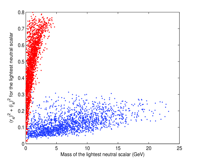
Figure 7: The $\Phi_{4}$ component of the lightest neutral scalar plotted against the mass of that scalar.

We next turn to the low-mass neutral scalar which is an—indirect—prediction of our model. We remind the reader that we have enforced on our points the condition that all scalars but one neutral one have mass larger than $100~{}\mathrm{GeV}$. Let $m_{\mathrm{light}}$ denote the mass of the lightest physical neutral scalar. In figure 7 we have plotted $m_{\mathrm{light}}$. We see in that figure that $m_{\mathrm{light}}\ \mbox{\raisebox{-3.0pt}{$\stackrel{{\scriptstyle\displaystyle<}}{{\sim}}$}}\ 25~{}\mathrm{GeV}$ for a normal neutrino mass spectrum, but $m_{\mathrm{light}}$ is much lower—$5~{}\mathrm{GeV}$ or less—in the case of an inverted neutrino mass spectrum.

Let $S_{\mathrm{light}}$ denote the light-scalar field; we write it as

$$S_{\mathrm{light}}=\sum_{j=1}^{4}\left[r_{j}\,\mathrm{Re}\left(\phi_{j}^{0}-v_{j}\right)+i_{j}\,\mathrm{Im}\left(\phi_{j}^{0}-v_{j}\right)\right],$$ (46)

where the $r_{j}$ and the $i_{j}$ are real and are normalized through

$$\sum_{j=1}^{4}\left[\left(r_{j}\right)^{2}+\left(i_{j}\right)^{2}\right]=1.$$ (47)

In the vertical axis of figure 7 we display the coupling of the low-mass scalar to $\Phi_{4}$. This is especially relevant since $\phi_{1,2,3}^{0}$ couple to neutrinos; only $\phi_{4}^{0}$ couples to $\bar{\alpha}_{L}\alpha_{R}$. Thus, if both $r_{4}$ and $i_{4}$ are small, then $S_{\mathrm{light}}$ has suppressed couplings to the charged leptons and may become invisible. One notices in figure 7 that cases with a normal neutrino mass spectrum usually display both a larger $m_{\mathrm{light}}$ and smaller $r_{4}$ and $i_{4}$ than cases with an inverted spectrum.

Moreover, in our model, just as in the Standard Model, the coupling of the neutral scalars to the charged leptons is suppressed by the charged-lepton mass, cf. equation (7). Now, as seen in figure 8, almost all our points have $\left|v_{4}\right|\>\mbox{\raisebox{-3.0pt}{$\stackrel{{\scriptstyle\displaystyle>}}{{\sim}}$}}\>\,20~{}\mathrm{GeV}$. Therefore, the coupling of $\phi_{4}^{0}$ to either $\bar{e}_{L}e_{R}$ or $\bar{\mu}_{L}\mu_{R}$ is always extremely small.

A possible discovery channel of the light scalar would have been through the process $e^{+}e^{-}\to Z^{0}S_{\mathrm{light}}$ at LEP. The LEP bound on this process only extends down to $m_{\mathrm{light}}\>\mbox{\raisebox{-3.0pt}{$\stackrel{{\scriptstyle\displaystyle>}}{{\sim}}$}}\>12~{}\mathrm{GeV}$, cf. table 14 of reference [13]. Another possible discovery channel for the light scalar would have been $e^{+}e^{-}\to Z^{\ast}\to S_{\mathrm{light}}S^{\prime}$, where $S^{\prime}$ is any neutral scalar heavier than $S_{\mathrm{light}}$—there are six possible $S^{\prime}$ in our model. In order to investigate these possibilities we have computed, for each of our points and for all seven physical scalars $S_{i}$, the strengths of the couplings $ZZS_{i}$ and $ZS_{i}S_{j}$. We have compared those strengths with the data in tables 14 and 19 of reference [13], which are the LEP bounds on $e^{+}e^{-}\to ZS_{i}$ and on $e^{+}e^{-}\to S_{i}S_{j}$, respectively, assuming that both $S_{i}$ and $S_{j}$ decay exclusively into $\tau^{+}\tau^{-}$; the second bound is effective for $m_{i}+m_{j}\ \mbox{\raisebox{-3.0pt}{$\stackrel{{\scriptstyle\displaystyle<}}{{\sim}}$}}\ 200$ GeV, the LEP kinematic limit. We have found that only a small percentage of our points (about 16% in the normal case, 10% in the inverted case) can be eliminated in this way. This is because, for most of our points, either the $S_{i}$ are much too heavy, thus kinematically evading the LEP bound, or the $S_{i}$ have much too small couplings (in many cases, zero for all practical purposes) to $ZS_{j}$; moreover, even when they are with the kinematic limits of LEP, the $S_{i}$ almost always have a minuscule coupling to $ZZ$. Remaking our plots by using only the points that have survived these tests, we have found that they look undistinguishable from the ones presented in figures 1–6. We remark that our tests are in all likelihood much too strict, since usually in our model the neutral scalars will not decay exclusively into $\tau^{+}\tau^{-}$.

Our $S_{\mathrm{light}}$ is not necessarily produced at the LHC through gauge-boson fusion, since it does not need to couple to the top quark—we remark that in this paper we have not specified the quark Yukawa couplings, which might even necessitate the addition to the model of extra Higgs doublets.

4 Summary

In this paper we have discovered that the $A_{4}$-symmetric renormalizable scalar potential for an $SU(2)\times U(1)$ gauge theory with one $A_{4}$ triplet of Higgs doublets, together with one $A_{4}$-invariant doublet, allows (local) minima for which two of the Higgs doublets in the $A_{4}$ triplet have equal VEVs. We have made use of such minima in a specific seesaw model with $A_{4}$ horizontal symmetry in the lepton sector. We have thus obtained a renormalizable model which makes the predictions (2) and (3) for the (effective) light-neutrino Majorana mass matrix $M$ in the basis where the charged-lepton mass matrix is diagonal. We have shown that those predictions are compatible with the phenomenological data on neutrino masses and mixings, irrespective of whether the neutrino mass spectrum is normal or inverted. Remarkably, we have found that in all such cases the scalar potential turns out to lead to (at least) one very light neutral scalar, with mass not larger than 25 (5) GeV in the cases with normal (inverted) neutrino mass spectrum.

Acknowledgements:

The work of L.L. is funded by the Portuguese Fundação para a Ciência e a Tecnologia (FCT) through FCT unit 777 and through the projects CERN/FP/116328/2010, PTDC/FIS/098188/2008, and PTDC/FIS/117951/2010, and also by the Marie Curie Initial Training Network “UNILHC” PITN-GA-2009-237920. The work of P.F. is supported in part by the Portuguese Fundação para a Ciência e a Tecnologia (FCT) under contract PTDC/FIS/117951/2010, by the FP7 Reintegration Grant n. PERG08-GA-2010-277025, and by PEst-OE/FIS/UI0618/2011.

Figure 1: Histogram displaying the distribution of the lowest neutrino mass, $m_{1}$, among the points with a normal neutrino mass spectrum. In our set of such points, $0.0021~{}\mathrm{eV}\leq m_{1}\leq 0.0277~{}\mathrm{eV}$.

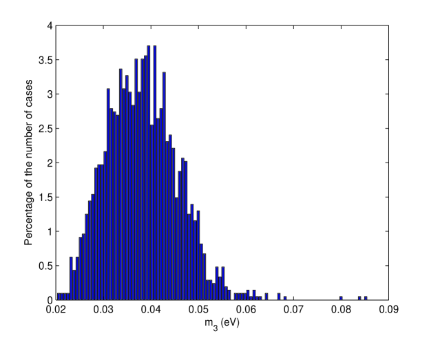
Figure 2: Histogram of the distribution of the lowest neutrino mass, $m_{3}$, in points with an inverted neutrino mass spectrum. For all those points $0.0203~{}\mathrm{eV}\leq m_{1}\leq 0.0855~{}\mathrm{eV}$.

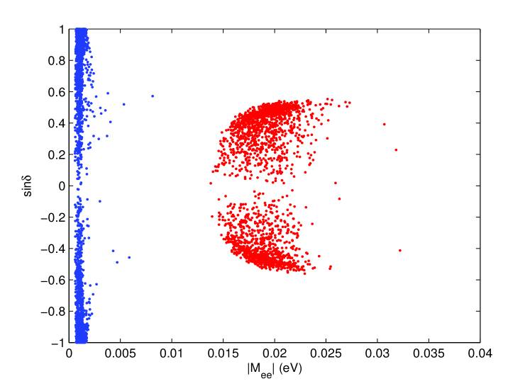
Figure 3: Scatter plot of the Dirac phase against $m_{2\beta 0\nu}$. Here and in the following figures, points with a normal neutrino mass spectrum are marked blue, those with an inverted spectrum are marked red.

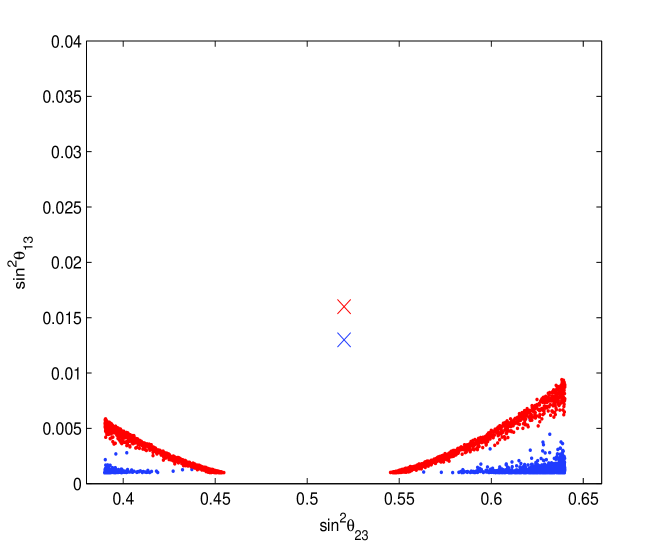
Figure 4: Scatter plot of the reactor angle $\theta_{13}$ against the atmospheric angle $\theta_{23}$. The crosses mark the best-fit points in table 1.

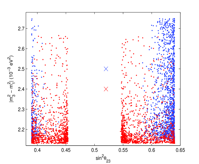
Figure 5: Fit of our model to the atmospheric-neutrino oscillations.

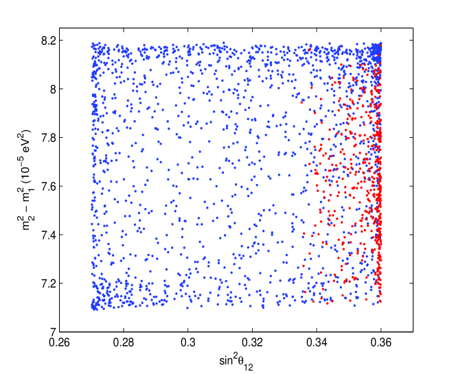
Figure 6: Fit of our model to the solar-neutrino oscillations.

Figure 8: The vacuum expectation value of $\phi_{4}^{0}$ plotted against the mass of the lightest neutral scalar.

References

- [1] T. Schwetz, M. Tórtola, and J. W. F. Valle, Where we are on : addendum to ‘Global neutrino data and recent reactor fluxes: status of three-flavor oscillation parameters’, New J. Phys. 13 (2011) 109401.
- [2] G. L. Fogli, E. Lisi, A. Marrone, A. Palazzo, and A. M. Rotunno, Evidence of from global neutrino data analysis, Phys. Rev. D 84 (2011) 053007.
- [3] G. Altarelli and F. Feruglio, Discrete flavor symmetries and models of neutrino mixing, Rev. Mod. Phys. 82 (2010) 2701.
- [4] Two useful papers explaining the features and advantages of are E. Ma, Plato’s fire and the neutrino mass matrix, Mod. Phys. Lett. A 17 (2002) 2361; E. Ma, symmetry and neutrinos, Int. J. Mod. Phys. A 23 (2008) 3366.
- [5] Some papers (among many others) using horizontal symmetry are G. Altarelli and F. Feruglio, Tri-bimaximal neutrino mixing from discrete symmetry in extra dimensions, Nucl. Phys. B 720 (2005) 64; G. Altarelli and F. Feruglio, Tri-bimaximal neutrino mixing, , and the modular symmetry, Nucl. Phys. B 741 (2006) 215; E. Ma, Dark scalar doublets and neutrino tribimaximal mixing from symmetry, Phys. Lett. B 671 (2009) 366; E. Ma, Neutrino tribimaximal mixing from alone, Mod. Phys. Lett. A 25 (2010) 2215; E. Ma and D. Wegman, Nonzero for neutrino mixing in the context of symmetry, Phys. Rev. Lett. 107 (2011) 061803.
- [6] P. H. Frampton, S. L. Glashow, and D. Marfatia, Zeroes of the neutrino mass matrix, Phys. Lett. B 536 (2002) 79.
- [7] L. Lavoura, Zeros of the inverted neutrino mass matrix, Phys. Lett. B 609 (2005) 317.
- [8] M. Hirsch, S. Morisi, E. Peinado, and J. W. F. Valle, Discrete dark matter, Phys. Rev. D 82 (2010) 116003.
- [9] R. de A. Toorop, F. Bazzocchi, L. Merlo, and A. Paris, Constraining flavour symmetries at the EW scale I: the A4 Higgs potential, JHEP 1103 (2011) 035.
- [10] L. Lavoura and H. Kühböck, model for the quark mass matrices, Eur. Phys. J. C 55 (2008) 303.
- [11] In http://www.interactions.org/cms/?pid=1031513
- [12] R. de A. Toorop, F. Bazzocchi, L. Merlo, and A. Paris, Constraining flavour symmetries at the EW scale II: the fermion processes, JHEP 1103 (2011) 040.
- [13] S. Schael et al. (ALEPH, DELPHI, L3, and OPAL Collaborations and the LEP Working Group for Higgs Boson Searches), Search for neutral MSSM Higgs bosons at LEP, Eur. Phys. J. C 47 (2006) 547.