Diagnosing the top-quark angular asymmetry
using LHC intrinsic charge asymmetries

Abstract

Flavor-violating interactions involving new heavy particles are among proposed explanations for the $t\bar{t}$ forward-backward asymmetry observed at the Tevatron. Many of these models generate a $t\bar{t}$-plus-jet signal at the LHC. In this paper we identify several new charge asymmetric variables in $t\bar{t}j$ events that can contribute to the discovery of such models at the LHC. We propose a data-driven method for the background, largely eliminating the need for a Monte Carlo prediction of $t\bar{t}$-plus-jets, and thus reducing systematic errors. With a fast detector simulation, we estimate the statistical sensitivity of our variables for one of these models, finding that charge-asymmetric variables could materially assist in the exclusion of the Standard Model across much of the mass and coupling range, given 5 inverse fb of data. Should any signal appear, our variables will be useful in distinguishing classes of models from one another.

I Introduction

The most peculiar among the Standard Model fermions, the top quark has challenged the high energy physics community, both on the experimental and theoretical level, since its discovery in 1995. From the theoretical viewpoint, its exceptional mass suggests that it might play a special role in the mechanism of electroweak symmetry breaking. This occurs in a number of proposed theories, including Little Higgs and Top-color Assisted Technicolor, and even within many supersymmetric models. On the experimental side, the predictions of the Standard Model (SM) for the top quark are still not fully tested. At the Tevatron, the high production threshold limited the number of $t\bar{t}$ events, and only now at the LHC will it be possible to perform precision measurements of the top quark’s properties.

While most aspects of the top quark agree so far with SM predictions, both the CDF Aaltonen:2011kc ; CDFLeptons and D0 Abazov:2011rq ; :2007qb collaborations have reported an anomalous forward-backward asymmetry for $t\bar{t}$ pairs at intermediate to high invariant mass, much larger than expected from SM calculations Kuhn:1998jr ; Kuhn:1998kw ; Bowen:2005ap ; Almeida:2008ug ; Ahrens:2011uf ; Kuhn:2011ri . This result, which relies upon “forward” being defined relative to the Tevatron’s proton beam, cannot be immediately checked at a proton-proton collider such as the LHC. However, it is well-known that forward-backward asymmetries at a proton-antiproton machine lead to differential charge asymmetries at a proton-proton machine, and indeed, a differential charge asymmetry in $t\bar{t}$ production, as a function of the $t$ quark’s rapidity, should be observable. This quantity has been discussed by theorists, for instance in Langacker:1986 ; Dittmar:1996my ; Li:2009xh ; Wang:2010tg ; Jung:2011zv ; Hewett:2011wz , and has been measured at the LHC experiments ATLASChargeAsymm ; CMSChargeAsymmearly ; CMSChargeAsymm . The statistical errors on this measurement are still rather large, however, and meanwhile the LHC’s higher energy allows its experiments to probe for related phenomena in other ways.

No significant problems with the SM calculation or the experimental measurements of the anomalously large asymmetry have been found. Meanwhile, a variety of models have been proposed to explain it. Most of these produce the asymmetry through the exchange of a new particle, either an $s$-channel mediator with axial couplings to both top and light quarks Sehgal:1987wi ; Bagger:1987fz ; Djouadi:2009nb ; Ferrario:2009bz ; Frampton:2009rk ; Chivukula:2010fk ; Bauer:2010iq ; Chen:2010hm ; Alvarez:2010js ; Delaunay:2011vv ; Bai:2011ed ; Barreto:2011au ; Foot:2011xu ; Zerwekh:2011wf ; Haisch:2011up ; Barcelo:2011fw ; Barcelo:2011vk ; Gabrielli:2011jf ; Tavares:2011zg ; Alvarez:2011hi ; AguilarSaavedra:2011ci , or a $t$-channel (or $u$-channel) mediator Jung:2009jz ; Cheung:2009ch ; Shu:2009xf ; Arhrib:2009hu ; Dorsner:2009mq ; Barger:2010mw ; Xiao:2010hm ; Cheung:2011qa ; Shelton:2011hq ; Berger:2011ua ; Grinstein:2011yv ; Patel:2011eh ; Craig:2011an ; Ligeti:2011vt ; Jung:2011zv ; Buckley:2011vc ; Nelson:2011us ; Duraisamy:2011pt ; Cao:2011hr ; Stone:2011dn with flavor-violating couplings that convert a light quark or antiquark to a top quark. Both processes are illustrated in Fig. 2. In Jung:2009pi ; Cao:2009uz ; Cao:2010zb ; Jung:2010yn ; Jung:2010ri ; Choudhury:2010cd ; Delaunay:2011gv ; Gresham:2011pa ; Shu:2011au ; Gresham:2011fx ; Westhoff:2011tq ; Berger:2011 , comparisons between different models are carried out, and study of those models or measurements in the LHC context can be found in Gresham:2011dg ; Blum:2011up ; AguilarSaavedra:2011vw ; Hewett:2011wz ; AguilarSaavedra:2011hz ; AguilarSaavedra:2011ug ; Jung:2011id ; Kahawala:2011sm ; Berger:2011xk ; Grinstein:2011dz ; Berger:2011sv ; Falkowski:2011zr .

Charge asymmetries at the LHC are known to be powerful tools for searching for and studying new physics, and recently this has been put to use in the context of models for the $t\bar{t}$ asymmetry. In Craig:2011an a large overall charge asymmetry was used to argue the Shelton-Zurek model Shelton:2011hq was most likely excluded; a similar method was then applied for a different model in Rajaraman:2011rw . Here, we focus on models with $t$- or $u$-channel mediators, which, as we will see, often generate large charge asymmetries in $t\bar{t}j$ (top plus antitop plus a jet) at the LHC. These asymmetries, a smoking gun of this type of model, will be crucial for a convincing discovery or exclusion of this class of models. Note these asymmetries are not directly related to the Tevatron forward-backward asymmetry in $t\bar{t}$ events, which translate at the LHC into the differential charge asymmetry in $t$ production mentioned above. The asymmetry in $t\bar{t}j$ that we study here stems from a completely different source; see below.

Any of the models with a $t$- or $u$-channel mediator has a coupling between a light quark or antiquark, a top quark, and a new particle $X$, as in Fig. 1(b). It follows that the $X$ can be produced from an off-shell quark or antiquark in association with a $t$ or $\bar{t}$, as shown in Fig. 2. Consequently, as has been pointed out by many authors Shu:2009xf ; Dorsner:2009mq ; Cheung:2011qa ; Gresham:2011dg ; Shu:2011au ; Berger:2011xk , it is important at the LHC to look for the process $pp\to Xt$ (and the conjugate process $pp\rightarrow\bar{X}\bar{t}$), where $X$ in turn decays to $\bar{t}$ plus a jet. A straightforward search for a $t$+jet resonance can be carried out, though it suffers from the poor resolution for reconstructing the resonance, large intrinsic backgrounds whose shape may peak near the resonance mass, and combinatoric backgrounds in the reconstruction. Alternatively, one could attempt a cut-and-count experiment; with appropriate cuts one can obtain samples in which the $X$ production contributes a statistically significant excess to the $t\bar{t}j$ rate. But the $t\bar{t}j$ background is not simple to model or measure, and systematic errors may be problematic.

(a) s-channel

(b) t-channel

Figure 1: Diagrams that can lead to a forward-backward asymmetry at the Tevatron in $t\bar{t}$ production. The $X$ is exchanged either (not both) in the $s-$ or $t-$/$u-$channel. $q$ may be $u$ or $d$.

Figure 2: For a $t$- or $u$-channel mediator $X$, direct production of $tX$ (followed by $X\to\bar{t}+q$ or $\bar{q}$) is always possible.

Fortunately, the process shown in Fig. 2 has a large charge asymmetry. The difference between quark and antiquark pdfs assures that the rate for $X$ production is different from that of $\bar{X}$ production. (If $X$ is self-conjugate, same-sign top-quark production results, and is readily excluded ATLASSameDiTop ; Chatrchyan:2011dk ; we therefore assume that $\bar{X}\neq X$.) Our approach in this work will be to suggest something a bit more sophisticated than a simple resonance search, using the charge asymmetries of these models to reduce systematic errors at a limited price in statistics. We will also propose other charge-asymmetric variables that can serve as a cross-check. As a by-product, should any discovery occur, the asymmetry itself can serve as a diagnostic to distinguish certain classes of models from one other.

II Benchmark Models

As our benchmark model, we take a typical model with a $t$-channel mediator, a colorless charged spin-one particle which we call a $W^{\prime}$. We will assume the $W^{\prime}$ couples a right-handed $d$ quark to a $t$ quark. While a theory with only these couplings would be inconsistent, we will assume this coupling generates the largest observable effects. One may say that we choose a “simplified model”, or “model fragment”, in which this coupling is the only one that plays an experimentally relevant role. We will see this point is not generally essential. The Lagrangian we take for our simplified model is simply

$$\mathcal{L}=-g_{R}W_{\mu}^{{}^{\prime}+}\bar{t}\gamma^{\mu}P_{R}d+h.c.$$ (1)

where $P_{R}=(1+\gamma^{5})/2$.

We are interested in the process in which the $W^{\prime}$ contributes to a $t\bar{t}j$ final state. One contribution comes from $dg\to tW^{\prime-}$ and its conjugate $\bar{d}g\to\bar{t}W^{\prime+}$, following which the $W^{\prime-}$ decays to $\bar{t}d$ and the $W^{\prime+}$ decays to $t\bar{d}$. We will refer to this as “$s$-channel production” (see Fig. 3). The $W^{\prime}$ also contributes to $dg\to t\bar{t}d$, and similar processes, through $t$-channel exchange (see Fig. 4).

(a) $W^{\prime-}$ production

(b) $W^{\prime+}$ production

Figure 3: Dominant production mode for the $W^{\prime}$. The cross-section for $W^{\prime-}$ is much larger than for $W^{\prime+}$.

The cornerstone of our analysis is the observation that in the $s$-channel process, the negatively charged $W^{\prime}$ is produced more abundantly than the positively charged $W^{\prime}$, because the negative $W^{\prime}$ can be produced from a valence quark, while a positive $W^{\prime}$ requires a sea antiquark in the initial state. (See Fig. 3.)

The processes in Figs. 3 and 4 can in principle have non-trivial interference with the Standard Model background — a point which considerably complicates background simulation. But we have found that interference is not numerically important for certain observables, at least with current and near-term integrated luminosities. All results in this paper therefore ignore interference; however, with larger data sets, or when studying other models and/or using other variables, one must confirm on a case-by-case basis that this approximation is sufficiently accurate for the analysis at hand.

Figure 4: Characteristic examples of diagrams that contribute to $t\bar{t}j$ production involving the $W^{\prime}$ in $t$-channel exchange.

In Cheung:2011qa , the authors studied this model and fitted it to the $t\bar{t}$ asymmetry and total cross-section in CDF. (This was done prior to the DZero result that shows a smaller asymmetry with less energy dependence.) Based on this work, we will take six benchmark points shown in Table 1, with three values of the $W^{\prime}$ mass and two values of $g_{R}$ for each mass, a larger value that would reproduce the CDF measurement and a value $\sqrt{2}$ smaller that would give a Tevatron asymmetry (and also an $W^{\prime}$ width and $tW^{\prime}$ production rate) of about half the size. The cross-sections at these benchmark points (including all the processes shown in Figs. 3 and 4) are also given in Table 1.

Mass (GeV)	$\>\>g_{R}\>\>$	cross-section (pb)
400	1.5	32.2
400	$\frac{1.5}{\sqrt{2}}$	12.9
600	2	18.2
600	$\sqrt{2}$	6.3
800	2	6.5
800	$\sqrt{2}$	2.1

Table 1: 7 TeV LHC tree-level cross-sections for the processes shown in Figs. 3 and 4, for the various benchmark points. No K-factor is included in these numbers, but we do apply one later in our analysis; for a discussion of the simulations and the K-factor, we refer the reader to Sec. IV.

The $W^{\prime}$ also contributes to $t\bar{t}$ production through $t$-channel exchange, and thus to the differential charge asymmetry in $t$ rapidity at the LHC (not to be confused with the asymmetries in $t\bar{t}j$ that are the subject of this paper.) ATLAS and CMS measurements of this quantity (with respectively 0.7 and 1.1 $\mathrm{fb}^{-1}$ of data) ATLASChargeAsymm ; CMSChargeAsymm may somewhat disfavor the benchmark points with the larger values of $g_{R}$, which (at parton-level, not accounting for $t$ reconstruction efficiencies) give a differential charge asymmetry in the 8–9% range. But the situation is ambiguous, since event mis-reconstruction and detector resolution produce a large dilution factor, which may make this charge asymmetry consistent with the current measurements. Our benchmarks with larger couplings thus probably represent the outer edge of what might still be allowed by the data. By considering also an intermediate coupling that still could explain the Tevatron $t\bar{t}$ asymmetry, we cover most of the interesting territory, and permit the reader to interpolate to other values of the couplings.

III A mass variable

Among the charge-asymmetric observables discussed in this paper, we will devote most of our attention to one motivated by the resonance structure of the $W^{\prime}$, which we will refer to as the mass variable $M_{j1bW}$ in later content. This variable is applicable universally to a wide range of $W^{\prime}$ masses and couplings, and to most other models with $tX$ production. We discuss this mass variable in great detail in this section. In Sec. VI, we will discuss the azimuthal angle between the hardest jet and the lepton (which we refer to as the “angle variable”.) A third class of potentially useful variables (“$P_{T}$ variables”), including the $P_{T}$ difference between the hadronic and the leptonic top quarks or $W$-bosons, is briefly discussed in Appendix C.

We will consider only the semi-leptonic $t\bar{t}j$ events (where one top decays hadronically and the other leptonically), resulting in a final state of 5 jets, a lepton and missing energy. All-hadronic decays are not useful for a charge asymmetry, as $t$ and $\bar{t}$ cannot be distinguished in this case, while the fully leptonic decay, though probably useful, has a low branching fraction.

Since it is the $s$-channel process in Fig. 3, where the $W^{\prime}$ appears as a resonance, that is charge-asymmetric, we will focus our attention there. In our later analysis we will impose an $S_{T}$ cut to improve the signal-to-background ratio. If we put that cut at $700$ GeV, the fraction of negatively charged $W^{\prime}$s for the 400, 600 and 800 GeV $W^{\prime}$ is $0.84$, $0.87$ and $0.86$ respectively. Such an enormous charge asymmetry in production can be put to good use.

Note, however, that since every event (following the $W^{\prime}$ decay) has a $t$ and a $\bar{t}$, either of which may produce the lepton, the total numbers of events with positively and negatively charged leptons are expected to be roughly equal, up to edge effects produced by cuts and detector acceptance. But since negative $W^{\prime}$s are produced more abundantly, a negatively charged lepton is more likely to come from the $W^{\prime}$ decay, while positive leptons tend to originate from the decay of the spectator top quark or antiquark. Kinematic features, such as the invariant mass and transverse mass of various final-state objects, differ for events with negatively and positively charged leptons. For instance, a simple bump hunt aimed at reconstructing the $W^{\prime}$ resonance would find a much larger bump in negatively charged leptons than in positively charged ones. Here, we will consider the $W^{\prime}$ reconstructed mass distribution more completely, noting that the signal remains asymmetric even away from the $W^{\prime}$ mass bump, since the total asymmetry must integrate to (almost) zero.

Another useful kinematical feature is that the hardest jet in $tW^{\prime}\to t\bar{t}d$ production commonly originates from the $d$-quark, because of the large energy released in the $W^{\prime}$ decay and the dissipation of the top quarks’ energies into their three daughters. At leading order and at parton-level, and with an $S_{T}$ cut of 700 GeV, the fraction of events where the hardest parton is the $d$-quark (or antiquark) from the $W^{\prime}$ is 0.71, 0.82 and 0.82 for a $W^{\prime}$ of mass 400, 600 and 800 GeV respectively. (Note neither ISR/FSR, hadronization, nor jet reconstruction are accounted for in these numbers, which are for illustration only.) We have designed our variables to maximally exploit these two kinematic features.

One conceptually simple approach to seeking the $W^{\prime}$ would involve fully reconstructing the $t$ and $\bar{t}$ in each event, and searching for a resonance in either $tj$ or $\bar{t}j$. This has been discussed in Shu:2009xf ; Dorsner:2009mq ; Cheung:2011qa ; Gresham:2011dg ; Shu:2011au ; Berger:2011xk . The challenge is that the combinatoric background is large and hard to model, and often peaks in a region not far from the resonance. Charge-asymmetries are useful here, because the positive-charge lepton events are dominated by the combinatoric background, while the negative-charge lepton events have similar combinatorics but a much larger resonance. Comparison of the two samples would allow for the elimination of a significant amount of systematic error.

However, full event reconstruction in events with five jets will have low efficiency, and moreover we are neither confident in our ability to model it nor certain it is the most effective method. Here we will instead focus on variables that require only partial event reconstruction. Of course the experimental groups should explore whether full event reconstruction is preferable to the methods we attempt here.

We will focus on the mass variable $M_{j1bW}$: the invariant mass of the hardest jet in the event, a $b$-tagged jet (chosen as described below), and a $W$-candidate reconstructed from the observed lepton and the missing transverse momentum (MET). It involves only a partial reconstruction of the event to form a candidate for the $W^{\prime}$, assuming it has decayed to a lepton. In signal events where the hardest jet in the event is a $d$ (or $\bar{d}$) from the $W^{\prime}$ decay, and the $\bar{t}$ (or $t$) from the $W^{\prime}$ produces a lepton $\ell$, $M_{j1bW}$ often reconstructs the $W^{\prime}$ resonance. The events with an $\ell^{-}$ typically exhibit a resonance at the $W^{\prime}$ mass, while those with an $\ell^{+}$, in which the $W^{\prime}$ is most often not reconstructed correctly, have a smoother distribution. This effect, and the resulting charge asymmetry — with a negative asymmetry near the $W^{\prime}$ mass and positive asymmetry elsewhere — are shown for $m_{W^{\prime}}=600$ GeV in Fig. 5. Both the asymmetric $s$-channel and the almost symmetric $t$-channel are included in what we call “signal.”

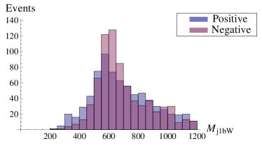
(a) $M_{j1bW}$ (parton-level) for signal only, shown for positive and negative lepton charge.

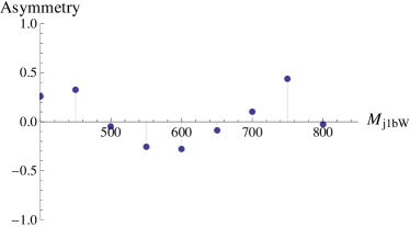
(b) Bin-by-bin signal-only charge asymmetry

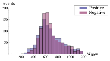
(c) $M_{j1bW}$ (parton-level) for signal plus background, shown for positive and negative lepton charge.

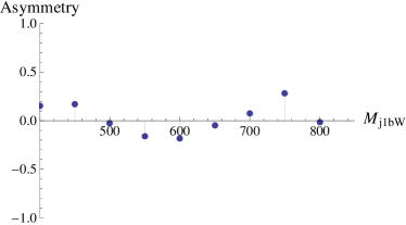
(d) Bin-by-bin signal plus background charge asymmetry

Figure 5: Parton-level charge asymmetry in the $M_{j1bW}$ variable for a 600 GeV $W^{\prime}$ with $g_{R}=2$ and an $S_{T}$ cut at 700 GeV. The leptonic $W$ boson was reconstructed from its decay products, $j_{1}$ was taken to be the hardest non-$b$ parton. ISR/FSR and $b$-quark selection effects were not accounted for here. The sample corresponds to 1.5 fb^-1.

In constructing $M_{j1bW}$, we reduce the combinatorial background by rejecting $b$-jets that are inconsistent with forming a top quark with the lepton and the MET ($M_{bl}<155$ GeV and $M^{T}_{bl\nu}<175$ GeV.) When multiple $b$-jets satisfy these criteria, we select the $b$-quark for which the quantity $|M_{bl}-155\>\mathrm{GeV}|+|M^{T}_{bl\nu}-175\>\mathrm{GeV}|$ is smallest. The combined efficiency of the $W$ reconstruction and the $b$ selection is about $45\%$.

Meanwhile, we will give evidence in Sec. V.1 that the SM background to this process shows no charge asymmetry in this variable, to a sufficiently good approximation. It is crucial for the use of this variable that this is true.

There are other invariant-mass and transverse-mass variables that have their merits. Some require no event reconstruction, including the invariant mass of the hardest jet and the lepton ($M_{j1l}$) and the invariant mass of the hardest jet, a $b$-tagged jet and the lepton ($M_{j1bl}$). For quantities that include the MET in the event, one could consider the transverse mass of two or more objects. (See also the footnote above concerning the hadronically decaying top in fully reconstructed events.) These variables and their charge asymmetries are strongly correlated, but one might still obtain additional sensitivity by combining them. But here, for simplicity, having found that the most sensitive variable on its own is $M_{j1bW}$, we will focus on it exclusively below.

IV Event selection and processing

We mentioned earlier that the $t\bar{t}j$ background and the $W^{\prime}$ signal do interfere with each other. However we have explicitly checked that interference effects do not alter the differential asymmetry in the $M_{j1bW}$ mass variable by a significant amount (given currently expected statistical uncertainties). The effect on the total number of events is also small. Thus it is relatively safe for us — and for the early searches at the LHC — to neglect interference in the study of the mass variable, at least for the $W^{\prime}$ model. (We have not studied whether this is true for all similar models with $tX$ production.) At some point, higher-precision study with much larger data samples ($\gg$ 10 fb^-1) may require the full set of interfering diagrams, and a special-purpose background-plus-signal simulation. Here we simulate background and signal independently.

On the other hand, $t$-channel $W^{\prime}$ exchange (Fig. 4) makes an important contribution to the cross-section and should always be included when generating the signal sample. (This is not uniformly the case in the literature.) For the variables we are studying, the $t$-channel process does not contribute much to the asymmetry, and effectively acts as an additional background.

A background sample and the signal samples for our benchmark points were generated with Madgraph 4.4.32 Alwall:2007st and showered with PYTHIA 6.4.22 Sjostrand:2006za . We performed a fast detector simulation with DELPHES 1.9 delphes . (For our parton-level studies the decays of the top and the antitop were simulated with BRIDGE 2.24 Meade:2007js ). We used the anti-$k_{T}$ jet-clustering algorithm (with $R=0.5$) to reconstruct jets. The isolation of leptons and jets is described in Appendix B.1. The $b$-tagging was modeled after the SV050 tagger of the ATLAS collaboration btag . We account for the rising $P_{T}$-dependence of the $b$-tagging efficiency, which reaches up to $60\%$ in the kinematic regime of interest. The dependence of the $b$ tagging efficiency on the pseudo-rapidity is assumed to be negligible within the $\eta$ reach of the tracker ($|\eta|<2.4$), with the tagging rate taken to be zero outside the tracker. The $c$-tag efficiency was assumed a factor of 5 smaller and the mistag rate is taken to be $1\%$. We do not account for the falloff in efficiency and the rise in mistag rates at higher $P_{T}$, since measurements of these effects are not publicly available; our tagging might therefore be optimistic, though the issue affects both signal and background efficiency.

We impose the following criteria for our event selection:

• At least 5 jets with $P_{T}^{jet}>30$ GeV and $|\eta|<5$

• At least one of these jets is $b$-tagged

• One isolated lepton ($e^{\pm}$ or $\mu^{\pm}$) with $P_{T}^{\ell}>30$ GeV and $|\eta|<2.5$

• MET $>30$ GeV.

where $\eta$ stands for pseudo-rapidity as usual. We also impose a cut on $S_{T}$, which is defined as

$$S_{T}=\sum P_{T}^{jet}+P_{T}^{\ell}+\mathrm{MET}$$ (2)

where the sum runs over all the jets with $P_{T}^{jet}>30$ GeV. The $S_{T}$ cut will be at a high enough scale (typically 600-800 GeV) that our events will pass the trigger with high efficiency.

The SM background simulation requires a matched sample for

$$p+p \rightarrow t+\bar{t}$$

$$p+p \rightarrow t+\bar{t}+j$$

where we use the MLM scheme Caravaglios:1998yr , with QCUT$=30$ and xqcut$=20$. The renormalization and factorization scales are set to $m_{T}$, where $m_{T}^{2}$ is the the geometric mean of $m_{t}^{2}+p_{T}^{2}$ for the top and antitop.

One might wonder whether it is necessary to include $pp\to t\bar{t}jj$ as well. But we are requiring 5 hard jets, and the mass and angle variables we will study are not sensitive to soft radiated jets, as they involve the hardest jet and a $b$-tagged jet. It is sufficient, therefore, for us to truncate our matched sample with one jet, and allow PYTHIA to generate any additional radiation. In total, we generated 3 million background events before matching. After matching, we find an inclusive $t\bar{t}$ LO cross-section of about 90 pb, so we include a K-factor of 1.7 to match with the NLO+NNLL QCD calculation Ahrens:2011mw ; QCDNLO . The number of events we generated for background corresponds to about 14 $\mathrm{fb}^{-1}$, large enough to provide smooth distributions for the variables we study.

There are a number of SM processes whose total cross-sections for producing a lepton are intrinsically charge-asymmetric. These include single-top production and $W$-plus-jets, for which an $\ell^{+}$ is more likely than an $\ell^{-}$. However, these have small rates for 5 jets and a lepton, especially with a $b$ tag required and with a hard $S_{T}$ cut. Moreover, asymmetries from any such process would be quite different from the signal, being both structureless and everywhere positive. We foresee no problem with such backgrounds.

For each value of the $W^{\prime}$ mass and coupling constant, we generated a signal sample with 750,000 events. No matching was used; extra ISR/FSR jets were generated by PYTHIA. These samples are large enough to suppress statistical fluctuations when we later use them to study the expected shape and magnitude of the asymmetry. In our studies, we have chosen to scale all LO signal cross-sections, for all six benchmark points, by a K-factor of 1.7, the same as for the $t\bar{t}$ background. Note that this K-factor can always be absorbed in $g_{R}$, as long as the width of the $W^{\prime}$ is smaller than the resolution.

V Analysis and results

Although the parton-level charge asymmetries described in Sec. III are large, the experimentally observable asymmetries are significantly diluted by the detector resolution and mis-reconstructions. Fig. 6(d) shows our estimate of the asymmetry structure that can be obtained at the detector level; compare this with Fig. 5. Note, however, that the basic structure of a negative asymmetry at the $W^{\prime}$ peak, with a positive asymmetry to either side, remains intact.

(a) $M_{j1bW}$ for a 400 GeV $W^{\prime}$, $g_{R}=1.5$

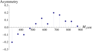
(b) Bin-by-bin asymmetry for a 400 GeV $W^{\prime}$, $g_{R}=1.5$

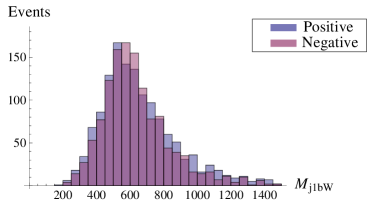
(c) $M_{j1bW}$ for a 600 GeV $W^{\prime}$, $g_{R}=2$

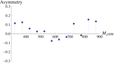
(d) Bin-by-bin asymmetry for a 600 GeV $W^{\prime}$, $g_{R}=2$

(e) $M_{j1bW}$ for an 800 GeV $W^{\prime}$, $g_{R}=2$

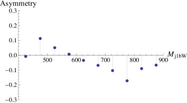
(f) Bin-by-bin asymmetry for an 800 GeV $W^{\prime}$, $g_{R}=2$

Figure 6: As in Fig. 5, but after accounting for detector effects, and with an $S_{T}$ cut of 700 GeV, for three different $W^{\prime}$ masses. All plots show signal plus background. The samples correspond to an integrated luminosity of 5 $\mathrm{fb}^{-1}$.

As always, one needs to obtain a prediction for both the Standard Model-only assumption (SM) and the Standard Model plus new physics assumption (NP), and assign a degree of belief to one or the other using a suitable statistical procedure, given the observed data. We will argue below that the SM prediction for the asymmetry in $M_{j1bW}$ is essentially zero, within the statistical uncertainties of the measurement. However, to predict the asymmetry in the presence of a signal requires a prediction of its dilution by the background. The background is also needed in order to predict the size of the fluctuations of the SM asymmetry around zero.

Direct use of Monte Carlo simulation to model the SM background distribution would be a source of large systematic errors, as NLO corrections are not known, and since we impose a hard cut on $S_{T}$. We therefore propose a (partially) data-driven method, minimizing this systematic error while keeping the statistical errors under control. The result can then be combined with a signal Monte Carlo to predict the differential asymmetry in $M_{j1bW}$. The search for a signal will then involve fitting this expectation to the data.

Our first task is to discuss how to obtain the prediction (which we will refer to as a “template”) for the differential asymmetry in $M_{j1bW}$, under both the SM and NP assumptions. We will begin by arguing that the SM asymmetry template is zero to a sufficiently good approximation. Next we will make a proposal for a partially data-driven method to determine the template for a given NP assumption, with low systematic uncertainty. Finally, we will estimate the sensitivity of our variables, using a simplified statistical analysis based in part on our proposed method. Along the way we will find the preferred value of the $S_{T}$ cut.

V.1 The SM Template: Essentially Zero

It is crucial for our measurement that the asymmetry in the SM background be known, so that the presence of a signal can be detected. It would be even better if the SM asymmetry is very small. Here we give evidence that this is indeed the case.

It is essential to recognize that the SM background to the $t\bar{t}j$ process is very different from the SM background to the $t\bar{t}$ process. In $t\bar{t}$, all asymmetries are zero at LO. The non-vanishing SM asymmetry in $t\bar{t}$ therefore arises from an NLO effect, involving both virtual corrections to $t\bar{t}$ and real emission, that is, $t\bar{t}j$. The asymmetry therefore cannot be studied at all with a leading-order event generator, and in a matched sample (which contains $t\bar{t}j$ but not the virtual correction to $t\bar{t}$) it would actually have the wrong sign.

However, for $t\bar{t}j$ itself, differential charge asymmetries at LO are not zero. The correction to these asymmetries from NLO corrections to $t\bar{t}j$ are subleading in general. Therefore we can ask the following question of an LO generator: although the generic observable in $t\bar{t}j$ events will show a charge asymmetry, is this the case for the $M_{j1bW}$ variable, or is any asymmetry washed out?

We find that the asymmetry in the mass variable is consistent with zero, as one can see in Fig. 7. This also turns out to be true for the angle variable which we will discuss later. We emphasize that this was not guaranteed to be the case. One can find variables that, at LO and at parton-level, exhibit asymmetries. An example is the asymmetry between the $P_{T}$ of the $t$ and that of the $\bar{t}$, which is of order 4% at parton-level. The fact that $qg\to t\bar{t}j$ has rather small asymmetries, and that the symmetric $gg$ initial state contributes significantly to $t\bar{t}j$, helps to reduce the size of any observable asymmetries. After reconstruction and detector effects, nothing measurable remains.

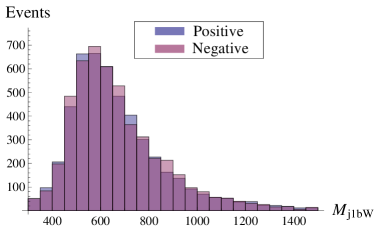
(a) $M_{j1bW}$ for SM background with a 700 GeV $S_{T}$ cut.

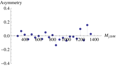
(b) Bin-by-bin asymmetry in $M_{j1bW}$ for SM background with a 700 GeV $S_{T}$ cut.

Figure 7: A parton-level study of the SM background asymmetry for the mass variable with a 700 GeV $S_{T}$ cut, corrsponding to 12 $\mathrm{fb}^{-1}$ luminosity. Other simulations confirm that the asymmetry appearing at 1200 – 1400 GeV is a statistical fluctuation.

We know of no reason why NLO corrections would change this conclusion. Neither virtual corrections nor real jet emission have any reason to strongly affect $M_{j1bW}.$ For this reason we will treat the SM background as purely symmetric.

No argument of this type is airtight. Fortunately, the experiments do not need to rely entirely upon it. As we see in Fig. 6(d), the asymmetry in the signal has a characteristic kinematic structure. Moreover, related asymmetries will show up in several mass variables in a correlated way, due to the $W^{\prime}$, and one would not expect similar correlations in the background. Finally, a signal is likely also to appear in the angle variable discussed in Sec. VI. The existence of these multiple cross-checks should allay any concerns that a measurement of a non-zero asymmetry might be uninterpretable.

V.2 Obtaining NP Templates and Accounting for Fluctuations

We now discuss how to obtain the NP template that is needed for each benchmark point. In addition one needs to be able to estimate the fluctuations that can occur under both the SM and NP assumptions. We emphasize the possibility of data-driven approaches.

$B^{+}_{i}\>(B^{-}_{i})$	Number of positive (negative) lepton events in $i^{th}$ bin, for background-only Monte Carlo.
$S^{+}_{i}\>(S^{-}_{i})$	As above, for signal-only Monte Carlo.
$D^{+}_{i}\>(D^{-}_{i})$	As above, in observed data.
$[D^{+}_{i}]\>([D^{-}_{i})]$	As above, in a fit to the observed data.
$\hat{A}_{i}$	Predicted charge asymmetry the $i^{th}$ bin for a particular hypothesis.
$A_{i}$	Charge asymmetry in $i^{th}$ bin as observed in data.
$c_{n}$	Amplitude for best fit of an NP template to the $n^{th}$ pseudo-experiment under the SM hypothesis.
$\tilde{c}$	Amplitude for best fit of an NP template to the asymmetry observed in the data.
$\sigma_{c}$	Standard deviation of the $c_{n}$.

Table 2: Notation used throughout Sec. V.

We will find it useful to introduce some notation (summarized in Table 2) in which $S^{\pm}_{i}$ and $B^{\pm}_{i}$ represent, for a signal-only and background-only Monte Carlo sample, the number of events in bin $i$ with a positively- or negatively-charged lepton $\ell^{\pm}$. $D^{\pm}_{i}$ denotes the similar quantity in data (and is thus not generally equal to the expected result $S^{\pm}_{i}+B^{\pm}_{i}$.) At some point we will need a smoothed version of the data, which we denote via $[D^{\pm}_{i}]$. The differential charge asymmetry predicted by the template for a particular benchmark point, or by the SM itself, we denote by $\hat{A}_{i}$. Meanwhile, we call the observed asymmetry in the data $A_{i}$.

Let us first focus on the statistical fluctuations around the template for the SM, which as we argued above in Sec. V.1 can be taken to be zero. Whenever one needs this template, it is under the assumption that the data is pure SM. Even without signal, there will be plenty of data with $\geq$ 5 fb^-1 and an $S_{T}$ cut of order 700 GeV. It therefore appears that rather than obtain the fluctuations around zero using a Monte Carlo sample $B_{i}$, one would have much smaller systematic errors using the data $D_{i}=D_{i}^{+}+D_{i}^{-}$ itself. One could probably do even better using a fit $[D_{i}]$ to the data, smoothing the bin-by-bin fluctuations in the numbers of events. We believe that the remaining statistical uncertainties that come with this method of modeling background will be smaller than the systematic uncertainties on an LO Monte Carlo for $B_{i}$. From this data-driven model, one may determine the expected size of the fluctuations on $\hat{A}_{i}$ by performing a series of pseudo-experiments.

Next let us consider how to determine the template $\hat{A}^{i}$ for a particular NP hypothesis We could of course simply compute it from large Monte Carlo samples, with Monte Carlo integrated luminosity $\mathcal{L}_{MC}$ much larger than the integrated luminosity in data $\mathcal{L}_{data}$, for $S_{i}$ and $B_{i}$.

$$\hat{A}_{i}\equiv\frac{S_{i}^{+}-S_{i}^{-}}{S_{i}^{+}+S_{i}^{-}+B_{i}^{+}+B^{-}_{i}}$$ (3)

(Recall we are ignoring interference for now.) Here the $B_{i}^{\pm}$ cancel in the numerator, since the asymmetry in the SM background is assumed to be zero. With this approach statistical errors can be made arbitrarily small, but systematic errors on the SM background prediction could be very substantial. The process $t\bar{t}j$ has never previously been measured at these energies, and after the $S_{T}$ cut it is difficult to estimate how large the systematic errors might be. Moreover we know of no way to extract the $t\bar{t}j$ background reliably, in the presence of signal, without the potential for signal contamination.

An alternative purely data-driven approach would be to use the suitably-fitted charge-symmetric data $[D_{i}^{+}+D_{i}^{-}]$ in the denominator of (3). For the numerator one may take a large Monte Carlo sample for $S_{i}$, and scale it to the luminosity of the data sample, giving

$$\hat{A}_{i}\equiv\frac{(S_{i}^{+}-S_{i}^{-})\frac{\mathcal{L}_{data}}{\mathcal{L}_{MC}}}{[D^{+}_{i}+D^{-}_{i}]}$$ (4)

where again $\mathcal{L}_{data}$ and $\mathcal{L}_{MC}$ are the luminosities of the data and the signal Monte Carlo sample. This method introduces correlations between the prediction of the template $\hat{A}^{i}$ and the measurement $A^{i}$ which would have to be studied and accounted for. However, the systematic error introduced by these correlations may in many cases be much smaller than those introduced by relying on a Monte Carlo simulation for the denominator, as in (3). In addition, statistical errors that arise from the finite amount of data, which would be absent with a large Monte Carlo sample, are negligible, as can be seen as follows. The statistical error on the predicted asymmetry $\hat{A}_{i}$ is dominated by fluctuations of the denominator of (4), since the statistical error on the numerator of (4) can be made arbitrarily small by increasing $\mathcal{L}_{MC}$:

$$\frac{\sigma(\hat{A}_{i})}{\hat{A}_{i}}=\frac{1}{[D^{+}_{i}+D^{-}_{i}]^{1/2}}.$$ (5)

However, for the measured asymmetry $A_{i}$, defined as $A_{i}\equiv\frac{D^{+}_{i}-D^{-}_{i}}{D^{+}_{i}+D^{-}_{i}}$, the error is always (for these models) dominated by the numerator:

$$\frac{\sigma(A_{i})}{A_{i}}=\frac{1}{(D^{+}_{i}+D^{-}_{i})^{1/2}}\sqrt{1+\frac{1}{A^{2}_{i}}}.$$ (6)

More precisely, since the largest observed asymmetries per bin will be of the order of $0.15$, the statistical error on the observed asymmetry is always larger than the statistical error on the template — $\sigma(A_{i})>>\sigma(\hat{A}_{i})$. And again we emphasize that this data-driven method reduces systematic uncertainties from what is often the largest source: the lack of confidence that the $t\bar{t}j$ background is correctly modeled. This comes at the relatively low cost of mild correlations between prediction and data, and some additional minor statistical uncertainty.

Partially data-driven approaches are also possible. Even if one uses $[D_{i}]$, the choice of fitting function could be determined in part with the use of Monte Carlos for $B_{i}$ and $S_{i}$. Interestingly, the distribution in the variable $M_{j1bW}$ is quite similar in signal and background, so the presence of signal, though it affects the overall rate, does not strongly affect the overall shape away from the $W^{\prime}$ resonance.

Since the pros and cons of these methods are luminosity-dependent, and dependent upon the details of the analysis, the only way to choose among these options is to do a study at the time that the measurement is to be made. We therefore do not attempt any optimization here. Whatever method is used, the last step in the process in obtaining the NP template is to fit the $\hat{A}_{i}$ to a smooth function, which then serves as the template for the asymmetry in this particular benchmark point. (The size of the fluctuations around this template can again be obtained from $[D_{i}]$, as we suggested for the SM template.) After repeating this process for a grid of benchmark points, one may then compare the data to the SM null template or to any one of the NP templates. In the next subsection we will carry out a simplified version of this study, to investigate the effectiveness of our methods.

V.3 Effectiveness of Our Method: A Rough Test

A full evaluation of our method, carrying out precisely the same analysis that the experimentalists will need to pursue, would require more firepower than we have available. Instead we will carry out a somewhat simplified analysis, asking the following question:

If the NP hypothesis for a certain benchmark point is realized in the data, what is the average confidence level at which we can reject the SM hypothesis?

The answer to this question will serve two purposes. First, it will give a measure of how sensitive a complete analysis will be for distinguishing the SM from various NP scenarios. (More precisely, it will be slightly optimistic, as we will discuss, but not overly so.) Second, it will allow us to estimate what value of the $S_{T}$ cut is optimal for different benchmark points.

We have not yet said much about the $S_{T}$ cut, so let us remark on it now. Without such a cut, the signal to background ratio in the $t\bar{t}j$ sample is small, as small as 1:45 for $m_{W^{\prime}}=800$ GeV with $g_{R}={\sqrt{2}}$. However, the situation can be much improved using the fact that the signal $S_{T}$ distribution tends (especially for heavy $W^{\prime}$s) to sit at much larger values for signal than for the SM background. (See Fig. 8; note these plots show the $S_{T}$ distributions for our large-$g_{R}$ benchmark points. From this one can see that a simple counting experiment would not be trivial.) The optimal value of the $S_{T}$ cut depends on the model, the analysis method and the luminosity. For most of our purposes an $S_{T}$ cut of the order of 700 GeV is suitable, as we will see later.

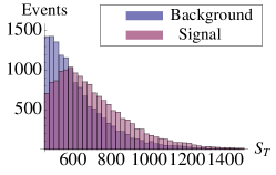
(a) $M_{W^{\prime}}=400\>\mathrm{GeV},\>g_{R}=1.5$

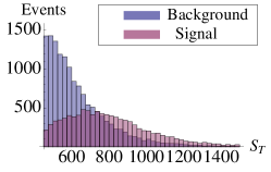
(b) $M_{W^{\prime}}=600\>\mathrm{GeV},\>g_{R}=2$

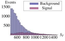
(c) $M_{W^{\prime}}=800\>\mathrm{GeV},\>g_{R}=2$

Figure 8: $S_{T}$ distributions of signal and background, for various benchmark points. For computational reasons we did not simulate events with $S_{T}<450$ GeV. The samples correspond to 8 fb^-1.

Answering the italicized question posed above is equivalent to evaluating the probability for fluctuations about the SM assumption to create a differential asymmetry $A_{i}$ that resembles the pattern predicted by the NP assumption $\hat{A}_{i}$. For this we need (a) the template $\hat{A}_{i}$ for the NP assumption and (b) an estimate of the size of the fluctuations that can occur under the SM assumption.

We have discussed above how to obtain these things from the data at the LHC. But since the actual data $D_{i}$ are not yet available, we obtain our NP template $\hat{A}_{i}$ from large $S_{i}$ and $B_{i}$ Monte Carlo samples, using formula (3). Obtaining the fluctuations under the SM assumption is a bit subtle. Since in this section we are assuming the data itself contains a signal, our background model must be obtained, according to our data-driven strategy, from our simulation of $S_{i}+B_{i}$ (and not from $B_{i}$ alone!) We take the expected numbers of positive- and negative-charge lepton events to both be equal to half of $S_{i}+B_{i}$. We then study the fluctuations around this background model by performing 50 000 Poisson-fluctuating pseudo-experiments, for positive- and negative-lepton events independently, and computing the differential asymmetry for each one.

Finally, to address our italicized question, we must then ask: what is the probability for fluctuations of the asymmetry around zero, given this background model, to resemble the “data”? This is done as follows: For each pseudo-experiment, we fit the differential asymmetry to the NP template $\hat{A}_{i}$ of our benchmark point, keeping the shape of the NP template fixed but allowing the amplitude to float. The best-fit amplitude we denote by $c_{n}$, where the index $n$ labels the pseudo-experiment. For illustration, some examples for a couple of pseudo-experiments are shown in Figs. 9(a) and 9(b).

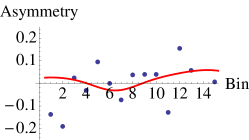
(a) SM pseudo-experiment, with amplitude $0.39$

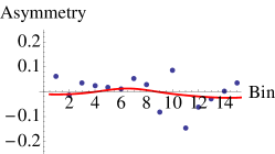
(b) SM pseudo-experiment, with amplitude $-0.16$

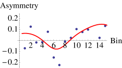
(c) NP pseudo-experiment, with amplitude $0.98$

Figure 9: Two examples of possible fluctuations of the differential charge asymmetry under the SM hypothesis, and one example under the NP hypothesis. The red line is the best fit of the amplitude of the NP template to the pseudo-experiment, with the shape held fixed. The NP template that was chosen corresponds to the 600 GeV $W^{\prime}$ with $g_{R}=2$ and $S_{T}>700$ GeV. The fluctuations are representative for a 5 $\mathrm{fb}^{-1}$ sample.

Under the SM assumption (zero asymmetry), the expectation value of the $c_{n}$ is zero. (Similarly, under the correct NP assumption, the expectation would be 1.) The $c_{n}$ follow a Gaussian distribution, whose width gives the standard deviation $\sigma_{c}$ of the $c_{n}$ around zero. If an amplitude of size $\tilde{c}$ were observed in the data, the $p$-value (chance of a fluctuation on the SM hypothesis to produce a structure with amplitude $\tilde{c}$ or larger) is then:

$$P[X>\tilde{c}]=\frac{1}{\sqrt{2\pi}\sigma_{c}}\int^{+\infty}_{\tilde{c}}\!\!\!\!\!\!dc\>e^{-\frac{1}{2}(c/\sigma_{c})^{2}}.$$ (7)

To get a measure of typical significance, we compute $P[X>1]$, the probability for the SM to produce an $A_{i}$ resembling the template $\hat{A}_{i}$ with an amplitude $\tilde{c}$ exceeding 1. (Recall that $\tilde{c}=1$ would be the expected value given that nature has chosen this benchmark point.) The results of this procedure for our benchmark points, after conversion to standard deviations on a Gaussian, are displayed in Table 3, for two integrated luminosities and for the optimal $S_{T}$-cut (see below.) In Appendix A, we also present contour plots of the significance as a function of the integrated luminosity and the $S_{T}$ cut; see Figs. 12 and 13.

The amount by which the observed significance tends to fluctuate around the expected significance depends on the luminosity and the $S_{T}$ cut. By running a different set of pseudo-experiments based on the NP hypothesis, we can obtain the Gaussian distribution of the amplitude of the fit. (An example of such a pseudo-experiment is shown in Fig. 9(c).) Values for the width of this distribution give us the statistical error bar on the expected significance, and are included in Table 3.

$\quad M_{W^{\prime}}\quad$ (GeV)	$\quad g_{R}\quad$	$\quad S_{T}$ cut (GeV)	Significance
			$\quad\quad 5\>\mathrm{fb}^{-1}\quad\quad$	$\quad\quad 8\>\mathrm{fb}^{-1}\quad\quad$
400	1.5	750	$6.27\pm 0.92$	$7.49\pm 0.75$
400	$\frac{1.5}{\sqrt{2}}$	750	$3.38\pm 0.95$	$4.24\pm 0.95$
600	2	700	$3.42\pm 0.92$	$4.08\pm 0.95$
600	$\sqrt{2}$	700	$1.79\pm 0.83$	$2.15\pm 0.86$
800	2	700	$2.37\pm 0.87$	$3.12\pm 0.92$
800	$\sqrt{2}$	700	$1.60\pm 0.82$	$2.01\pm 0.85$

Table 3: Expected significance and statistical error for SM exclusion at our benchmark points, given selected luminosities and optimal $S_{T}$ cuts. For the correct interpretation of these numbers, please refer to the text.

Our simplified analysis is imperfect in various ways. One important weakness is that we assume that nature matches one of our benchmark points, and we do not consider the effect of using the wrong benchmark point in obtaining the exclusion of the SM. In particular, the mass of the $W^{\prime}$ we used to obtain the NP template matches the mass of the $W^{\prime}$ in our “data”. A finer grid in $W^{\prime}$ mass would address this. (In general, the coupling $g_{R}$ for the template will also differ from the real coupling, but except for its effect on the $W^{\prime}$ width, often smaller than the experimental resolution, a change in the coupling affects the amplitude, but not the shape, of the corresponding template.) Also, our simplified procedure to fit only for the amplitude of the template and to keep the shape fixed does not always capture all the features of the asymmetry distribution, as is illustrated in Fig. 9(c), where the central dip in the asymmetry is deeper than our fit function can capture. In a more detailed study one might choose to let multiple parameters float to obtain a better fit. We further note that we are not accounting for the look-elsewhere effect. And finally, although the use of asymmetries and a data-driven method reduces systematic errors, we have not considered the remaining systematic errors here.

On the other hand, there are important features of the signal that we are not using in our analysis, and including those would enhance the sensitivity. The use of several (correlated) mass variables, and the angle variable discussed in the next section, would give some improvements. Moreover, while the charge asymmetry we focus on here has low systematic errors but is statistically limited, other observables with higher systematics but lower statistical errors, such as the differential cross-section with respect to $S_{T}$, are obviously useful as well. In any search for this type of models multiple approaches should be combined.

VI An angle variable

In this section we discuss another charge-asymmetric variable, the azimuthal angle between the hardest jet without a $b$-tag ($j_{1}$) and the lepton $\ell$:

$$\Delta\phi_{j_{1},\ell}=\mathrm{Min}\Big{[}|\phi_{j_{1}}-\phi_{\ell}|,\>2\pi-|\phi_{j_{1}}-\phi_{\ell}|\Big{]}.$$ (8)

With a low $S_{T}$ cut, the angle between the hardest jet and an $\ell^{-}$ tends to be larger than the angle between the hardest jet and an $\ell^{+}$ [Figs. 10(a) and 10(b)]. The reason is as follows: The $W^{\prime}$ is produced near threshold, so the recoiling top quark or antiquark is not highly boosted. The top from the $W^{\prime}$ decay, on the other hand, will recoil back-to-back against the $d$ or $\bar{d}$ (which is usually the source of the hardest jet). Moreover, this top will be somewhat boosted since $m_{W^{\prime}}\gg m_{t}$, so if it decays leptonically, the lepton’s momentum tends also to be back-to-back to the $d$ or $\bar{d}$. This results in a large opening angle between the hardest jet and the lepton. However, if it is the other top quark that decays leptonically, the angle of its lepton with the hardest jet is more randomly distributed. Since the negatively charged $W^{\prime}$ is produced more abundantly, this variable will exhibit a charge asymmetry.

For a high $S_{T}$ cut the picture reverses. The $W^{\prime}$ and the top from which it recoils are now both boosted and typically back-to-back with one other. The decay products from the $W^{\prime}$ tend to be aligned with each other. In other words, a cluster of four objects (from the $W^{\prime}$) is now recoiling against a cluster of three objects (the top). The hardest jet is typically still the down quark from the $W^{\prime}$ decay. If the lepton’s parent is the top from the $W^{\prime}$, $\Delta\phi_{j_{1}\ell}$ tends to be small, while the opposite is true if the lepton comes from the recoiling top. (See Figs. 10(c) and 10(d).)

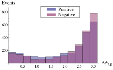
(a) The angle variable in signal only for $M_{W^{\prime}}=800$ GeV and $g_{R}=2$.

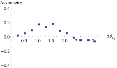
(b) Asymmetry of the angle variable in signal only for $M_{W^{\prime}}=800$ GeV and $g_{R}=2$.

(c) The angle variable in signal only for $M_{W^{\prime}}=400$ GeV and $g_{R}=1.5$.

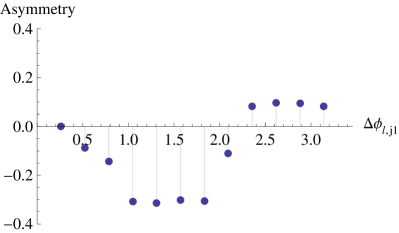
(d) Asymmetry of the angle variable in signal only for $M_{W^{\prime}}=400$ GeV and $g_{R}=1.5$.

Figure 10: Angle difference between the lepton and the hardest jet at parton-level signal-only, for $W^{\prime}$s of mass 800 and 400 GeV with an $S_{T}$ cut at 700 GeV. The samples correspond to 5 fb^-1.

This reversing structure in the asymmetry as a function of the $S_{T}$ cut is useful, as it potentially provides a very strong hint of new physics. However, there is an intermediate $S_{T}$ cut where the asymmetry is essentially zero, so in that range the variable is not useful. For this reason, we recommend studying this variable as a function of the $S_{T}$ cut.

We explicitly checked that the standard model will not introduce a large asymmetry in this angle variable, for any $S_{T}$ cut. A particular case is shown in Fig. 11. Our reasoning for trusting a LO Monte Carlo is the same as was described in Sec. V.1 for the mass variable.

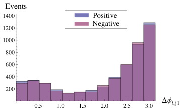
(a) The angle variable for SM background with a 700 GeV $S_{T}$ cut.

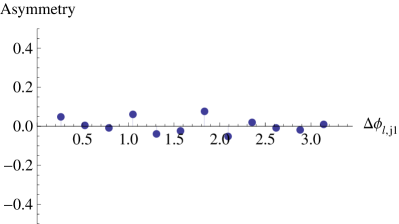
(b) Bin-by-bin asymmetry in the angle variable for SM background with a 700 GeV $S_{T}$ cut.

Figure 11: A parton-level study on SM background asymmetry for the angle variable with a 700 GeV $S_{T}$ cut, corresponding to 12 fb^-1 luminosity.

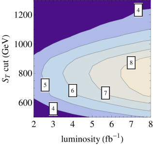
(a) $M_{W^{\prime}}=400$ GeV, $g_{R}=1.5$

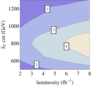
(b) $M_{W^{\prime}}=400$ GeV, $g_{R}=\frac{1.5}{\sqrt{2}}$

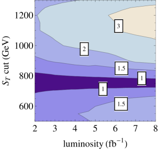
(c) $M_{W^{\prime}}=600$ GeV, $g_{R}=2$

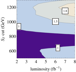
(d) $M_{W^{\prime}}=600$ GeV, $g_{R}=\sqrt{2}$

Figure 14: Expected significance of $\Delta\phi_{j_{1},\ell}$ for a 400 GeV and a 600 GeV $W^{\prime}$, as a function of luminosity and $S_{T}$ cut. For the 600 GeV $W^{\prime}$ the dark band corresponds to the range of $S_{T}$ cuts where the asymmetry is changing sign, which results in a much reduced sensitivity. Interference between signal and background is not accounted for.

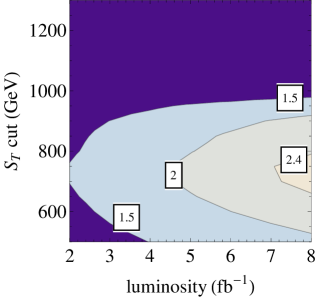
(a) $M_{W^{\prime}}=800$ GeV, $g_{R}=2$

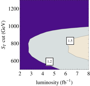
(b) $M_{W^{\prime}}=800$ GeV, $g_{R}=\sqrt{2}$

Figure 15: Expected significance of $\Delta\phi_{j_{1},\ell}$ for an 800 GeV $W^{\prime}$, as a function of luminosity and $S_{T}$ cut. Interference between signal and background is not accounted for.

An interesting feature of this angle variable in the $W^{\prime}$ model (though whether this is true in other models has not yet been studied) is that the point where the number of positive and negative lepton events is roughly equal is insensitive to $m_{W^{\prime}}$ and $g_{R}$. For all our benchmark points we find $\Delta\phi_{j_{1},\ell}\approx 2$ to be a suitable place to break the signal into two bins. The detector-level asymmetries in both bins are given in Table 4. To estimate the significance, we follow a strategy similar to the one mentioned for the mass variable. However instead of fitting for the amplitude of a previously obtained template, we compute the difference of the asymmetry of the two superbins and establish the Gaussian probability distribution for this variable using pseudo-experiments on the SM hypothesis. Plots of the resulting significance of this observable as a function of $S_{T}$ cut and luminosity can be found in Figs. 14 and 15 in Appendix A.

$\quad M_{W^{\prime}}\quad$ (GeV)	$\quad g_{R}\quad$	$\quad S_{T}$ cut (GeV)	Asymmetry (%)
			$\quad 1^{\mathrm{st}}$ bin	$\quad 2^{\mathrm{th}}$ bin
400	1.5	800	-13.7	10.2
400	$\frac{1.5}{\sqrt{2}}$	800	-9.3	7.0
600	2	1200	-9.6	12
600	$\sqrt{2}$	1200	-6.8	8.7
800	2	700	3.8	-2.4
800	$\sqrt{2}$	700	2.4	-1.7

Table 4: Expected asymmetry at detector-level in the angle variable for each superbin, for our benchmark points using the optimal $S_{T}$ cut.

The greatest merit of the angle variable is its simplicity. Both the hardest jet and the lepton are well-measured, and in contrast to the mass variables no (partial) event reconstruction is needed. Unfortunately the angle variable is more sensitive than $M_{j1bW}$ to interference effects between signal and background. Whether the contribution from interference is positive or negative depends on the mass of new particle, the $S_{T}$ cut and the model we study. The effect, however, appears to be only moderate. We find that, for a $W^{\prime}$ mass of 800 GeV and an $S_{T}$ cut of 700 GeV, the asymmetry for the two bins after interference is included is reduced by about 15%. A more detailed study including interference is advisable to give a precise estimate of its effects, especially for other models where interference might be more important.

VII Final Remarks

At the LHC, models that attempt to explain the Tevatron $t\bar{t}$ forward-backward asymmetry with the exchange of a particle $X$ in the $t$- or $u$-channel generate a charge-asymmetric signal in $tX$ production. This leads to observable charge asymmetries in certain variables within $t\bar{t}j$ samples. Among interesting observables are mass variables involving various final state objects including the hardest jet and/or the lepton (Secs. III and V), the azimuthal angle between the lepton and the hardest jet (Sec. VI) and the $P_{T}$ difference between the tops and $W$ bosons (Appendix C). Of these variables, the invariant mass of the hardest jet, the leptonic $W$ and a $b$-tagged jet appears to be the most powerful and the most universal, since it tends to reconstruct the $W^{\prime}$ mass resonance. The charge asymmetry of this variable exhibits a negative asymmetry in the region of the $W^{\prime}$ mass, and a positive asymmetry elsewhere. We have proposed a data-driven method to extract a statistical significance from this asymmetry structure.

One could of course go further by fully reconstructing the events, and directly observe that $W^{\prime-}$ production is larger than $W^{\prime+}$ production. However demanding full reconstruction would lead to a considerable loss of efficiency. Since we cannot realistically estimate this efficiency loss, we cannot evaluate the pros and cons of this approach, but clearly the experiments should do so.

We have described this asymmetry measurement on its own, without discussing the fact that simultaneously the experiments will be measuring charge-symmetric variables, such as the cross-section for $t\bar{t}j$ as a function of $S_{T}$. Of course these variables are complementary, and we do not in any way mean to suggest that one should do one instead of the other. Charge-symmetric variables may often have lower statistical uncertainties, but in most cases background-subtraction is necessary, so there will be large systematic errors. The combination of the two types of measurements will help clarify the situation far better than either one could in isolation. Additional information will come from the differential charge asymmetry in $t\bar{t}$ events at the LHC, which is a direct test of the Tevatron measurement of the $t\bar{t}$ forward-backward asymmetry, and is sensitive to any growth of the effect with energy.

A very important aspect of our approach is that the asymmetry is a diagnostic for models. An $s$-channel mediator will not generate a peak for either lepton charge, and so even if an asymmetry in $t\bar{t}j$ were generated, it would be largely washed out in the variable $M_{j1bW}$. Among models with $t$- or $u$-channel mediators $X$, some will produce a negative asymmetry at $M_{j1bW}=m_{X}$, while others will produce a positive asymmetry. For example, models that replace the $W^{\prime}$ by a color triplet or color sextet scalar $X$ Gresham:2011pa ; Shu:2011au ; Gresham:2011fx ; Westhoff:2011tq that couples to $u_{R}$ and $t_{R}$ (and has charge 4/3) will have the opposite sign, because the process $ug\rightarrow\bar{t}X^{+}$ will be larger than $\bar{u}g\rightarrow tX^{-}$. The approach we use will still apply, but the asymmetry will be positive in the neighborhood of the $X$ mass peak, rather than negative as it is for the $W^{\prime}$. For this reason, even if it turns out that the asymmetry measurement is not needed for a discovery of the $X$ particle, it will still be an essential ingredient in determining its quantum numbers and couplings.

What seems clear from our results is that the data already available (or soon to be available) at the 7 TeV LHC should be sufficient to allow for an informative measurement of charge-asymmetric observables in $t\bar{t}j$ to be carried out. We look forward to seeing studies of $t\bar{t}j$ from ATLAS and CMS, and we hope that measurements of charge asymmetries will be among them.

Appendix A Additional Results

A.1 Contour plots for the mass variable

As can be seen in Figs. 12 and 13, we find that the optimal $S_{T}$-cut for the mass variable does not vary greatly with luminosity, or even with the $W^{\prime}$ mass: it lies around $700$ GeV for the $600$ GeV and $800$ GeV $W^{\prime}$ and is slightly higher for the $400$ GeV $W^{\prime}$. At lower $S_{T}$ cuts, reduced signal-to-background ratio worsens the significance. The reason a large $S_{T}$ cut works well even for low $W^{\prime}$ mass is that the distribution for the charge-symmetric component of the signal (mainly $t$-channel $W^{\prime}$ exchange) peaks at low $S_{T}$ for a lighter $W^{\prime}$. Meanwhile, for an overly high $S_{T}$ cut the remaining signal is too small. But we should mention that our binning procedure makes our results too pessimistic here.

(a) $M_{W^{\prime}}=400$ GeV, $g_{R}=1.5$

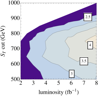
(b) $M_{W^{\prime}}=400$ GeV, $g_{R}=\frac{1.5}{\sqrt{2}}$

Figure 12: Expected significance of the $M_{j1bW}$ variable for a 400 GeV $W^{\prime}$, as a function of luminosity and $S_{T}$ cut.

When producing these contour plots, we choose a fixed binsize of 50 GeV everywhere except in the upper and lower tails of the distribution, where we use a superbin. The superbins are sized so that that no bin ever contains fewer than 50 events. For higher $S_{T}$, there are very few bins between the two superbins, and this makes the peak-valley-peak structure weak, ruining the significance of the measurement. Within the white region in the upper left of the plots, the number of events is so small that no bin with more than 50 events exists, and our binning strategy gives a null result. However, for a high $S_{T}$ cut one could choose a more sophisticated binning strategy. We have verified in a few particular cases that larger bins for higher $S_{T}$ cuts can restore some of the significance of the measurement. All of this is to say that sophisticated treatment of the data may lead to a somewhat better result than our simple-minded binning strategy would suggest.

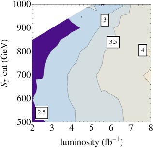
(a) $M_{W^{\prime}}=600$ GeV, $g_{R}=2$

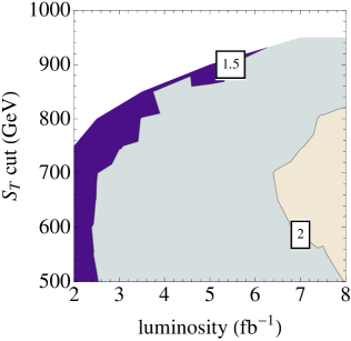
(b) $M_{W^{\prime}}=600$ GeV, $g_{R}=\sqrt{2}$

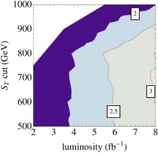
(c) $M_{W^{\prime}}=800$ GeV, $g_{R}=2$

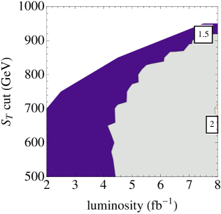
(d) $M_{W^{\prime}}=800$ GeV, $g_{R}=\sqrt{2}$

Figure 13: Expected significance of the $M_{j1bW}$ variable for a 600 GeV and an 800 GeV $W^{\prime}$, as a function of luminosity and $S_{T}$ cut.

A.2 Contour plots for the angle variable

The plots below show the significance for exclusion of the SM hypothesis using the angle variable, along the lines of our method used for the mass variable. Note the band of low significance for the $W^{\prime}$ with mass of 600 GeV, caused by the shifting structure that we emphasized in Sec. VI; for an $S_{T}$ cut of around 700 GeV, the asymmetry shifts from one sign to the other. A study exploiting this dependence of the asymmetry on the $S_{T}$ cut would have larger significance, but we have not explored this option here.

Appendix B Strategy Details

B.1 Isolation Procedure

The detector simulation DELPHES produces particle candidates and requires the user to impose the isolation criteria of his or her choice. Hence for each lepton candidate in the DELPHES output there will be a corresponding jet candidate, and it is up to the user to decide which one to include in the analysis. To facilitate this choice, DELPHES provides the user with the following variables for each lepton:

• $\Sigma P_{T}$: The sum of the $P_{T}$ of all the tracks with $P_{T}>0.9$ GeV in a cone of $\Delta R=0.3$ around the leading track, excluding that track.

• $\rho_{l}$: The sum of the energy deposited in a 3$\times$3 calorimeter grid around the leading track, divided by the $P_{T}$ of that track.

Here we lay out the isolation criteria we imposed on the various particle candidates. An isolated electron is defined as an electron candidate for which $\Sigma P_{T}<10$ GeV, $\Sigma P_{T}<0.15\>P_{T}^{e}$ and $\rho_{e}<1.15$. For isolated muons we require $\Sigma P_{T}<10$ GeV, $\Sigma P_{T}<0.15\>P_{T}^{\mu}$ and $\rho_{\mu}<0.15$. Finally jet candidates are retained if no isolated leptons are found in a cone of radius 0.3. When a previously isolated lepton is found in a 0.3 cone, the jet candidate is identified with the lepton and therefore removed from the event. We hereby impose two consistency conditions:

• No more than 1 isolated lepton is found in a 0.3 cone

• When one isolated lepton is found, the $P_{T}$ of the jet candidate can differ by no more than $10\%$ from the $P_{T}$ of the isolated electron.

When one of these criteria is not met, we are unable to carry out a consistent isolation procedure and the entire event is thrown out. The efficiency of our isolation procedure is $97\%$, both for signal and background samples.

Appendix C The $P_{T}$-difference variables

Among other variables that show charge-asymmetries, ones of possible further interest include the difference in $P_{T}$ between the $t$ and the $\bar{t}$, or between the positive and negative $W$ bosons.

Since one top quark is recoiling against the $W^{\prime}$, while the other top quark is a decay product of the $W^{\prime}$, one would expect their kinematics to differ. The $P_{T}$ difference between the $t$ and $\bar{t}$ is a variable in which this feature of the signal will manifest itself. The same is true for the $W$ bosons from the $t$ and $\bar{t}$ decays. For each event, we can calculate

$$\Delta P_{T,W}=\frac{P_{T,W^{+}}-P_{T,W^{-}}}{P_{T,W^{+}}+P_{T,W^{-}}}\quad\mathrm{and}\quad\Delta P_{T,t}=\frac{P_{T,t}-P_{T,\bar{t}}}{P_{T,t}+P_{T,\bar{t}}}.$$ (9)

The charge asymmetry at parton-level for these variables can be seen (for pure signal) in Figs. 16(a) and 16(b).

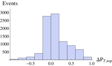
(a) Top $P_{T}$ difference in signal.

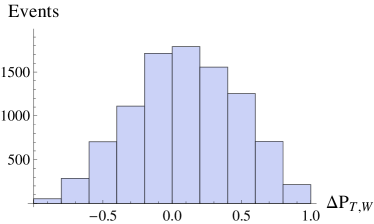
(b) W boson $P_{T}$ difference in signal.

Figure 16: Top quark and W boson $P_{T}$ difference at parton-level in signal with a 400 GeV $W^{\prime}$ with $S_{T}$ cut at 700 GeV. The sample is corresponding to a luminosity of 5 fb^-1.

Although spectacular at parton-level, we find that the $P_{T}$ difference between the top quarks gets washed out a lot at detector-level by resolution effects and mis-reconstructions. Nevertheless we encourage experimental colleagues to take this variable in consideration, since state-of-the-art top reconstruction methods might alleviate this problem. The $P_{T}$ difference between the $W$ bosons is less pronounced at parton-level, but does survive our detector simulation and the reconstruction of the hadronic $W$. We find it is particularly useful for a low mass $W^{\prime}$. Like the angle variable, it changes sign as a function of the $S_{T}$ cut.

We have not studied the effect of interference on these $P_{T}$ variables. Whether the asymmetry from the SM $t\bar{t}j$ background is important also requires further study.

References

- (1) CDF Collaboration , Phys. Rev. D83, 112003 (2011). [arXiv:1101.0034 [hep-ex]].
- (2) D0 Collaboration, [arXiv:1107.4995 [hep-ex]].
- (3) CDF Collaboration, CDF Note No. 10436
- (4) D0 Collaboration, Phys. Rev. Lett. 100, 142002 (2008). [arXiv:0712.0851 [hep-ex]].
- (5) J. H. Kuhn, G. Rodrigo, Phys. Rev. Lett. 81, 49-52 (1998). [arXiv:9802268 [hep-ph]].
- (6) J. H. Kuhn, G. Rodrigo, Phys. Rev. D59, 054017 (1999). [arXiv:9807420 [hep-ph]].
- (7) M. T. Bowen, S. D. Ellis, D. Rainwater, Phys. Rev. D73, 014008 (2006). [arXiv:0509267 [hep-ph]].
- (8) L. G. Almeida, G. F. Sterman, W. Vogelsang, Phys. Rev. D78, 014008 (2008). [arXiv:0805.1885 [hep-ph]].
- (9) V. Ahrens, A. Ferroglia, M. Neubert, B. D. Pecjak, L. L. Yang, [arXiv:1106.6051 [hep-ph]].
- (10) J. H. Kuhn and G. Rodrigo, [arXiv:1109.6830 [hep-ph]].
- (11) N. Kidonakis, PoSDIS 2010, 196 (2010) [arXiv:1005.3330 [hep-ph]].
- (12) ATLAS Collaboration, Technical Report ATLAS-CONF-2011-106, CERN, Geneva, Aug 2011
- (13) CMS Collaboration, CMS-PAS-TOP-10-010, CERN, Geneva, 2010.
- (14) CMS Collaboration, CMS-PAS-TOP-11-014, CERN, Geneva, 2011.
- (15) P. Langacker, R. W. Robinett, and J. L. Rosner, Phys. Rev. D30, 1470 (1984).
- (16) M. Dittmar, Phys. Rev. D 55, 161 (1997) [arXiv:9606002 [hep-ex]].
- (17) Y. Li, F. Petriello and S. Quackenbush, Phys. Rev. D 80, 055018 (2009) [arXiv:0906.4132 [hep-ph]].
- (18) Y. -K. Wang, B. Xiao, S. -H. Zhu, Phys. Rev. D83, 015002 (2011). [arXiv:1011.1428 [hep-ph]].
- (19) L. M. Sehgal, M. Wanninger, Phys. Lett. B200, 211 (1988).
- (20) J. Bagger, C. Schmidt, S. King, Phys. Rev. D37, 1188 (1988).
- (21) A. Djouadi, G. Moreau, F. Richard, R. K. Singh, Phys. Rev. D82, 071702 (2010), [arXiv:0906.0604 [hep-ph]].
- (22) P. Ferrario, G. Rodrigo, Phys. Rev. D80, 051701 (2009), [arXiv:0906.5541 [hep-ph]].
- (23) P. H. Frampton, J. Shu, K. Wang, Phys. Lett. B683, 294-297 (2010), [arXiv:0911.2955 [hep-ph]].
- (24) R. S. Chivukula, E. H. Simmons, C. -P. Yuan, Phys. Rev. D82, 094009 (2010), [arXiv:1007.0260 [hep-ph]].
- (25) M. Bauer, F. Goertz, U. Haisch, T. Pfoh, S. Westhoff, JHEP 1011, 039 (2010), [arXiv:1008.0742 [hep-ph]].
- (26) C. -H. Chen, G. Cvetic, C. S. Kim, Phys. Lett. B694, 393-397 (2011), [arXiv:1009.4165 [hep-ph]].
- (27) E. Alvarez, L. Da Rold, A. Szynkman, JHEP 1105, 070 (2011), [arXiv:1011.6557 [hep-ph]].
- (28) C. Delaunay, O. Gedalia, S. J. Lee, G. Perez and E. Ponton, Phys. Lett. B 703, 486 (2011) [arXiv:1101.2902 [hep-ph]].
- (29) Y. Bai, J. L. Hewett, J. Kaplan, T. G. Rizzo, JHEP 1103 (2011) 003. [arXiv:1101.5203 [hep-ph]].
- (30) E. R. Barreto, Y. A. Coutinho, J. Sa Borges, Phys. Rev. D83, 054006 (2011), [arXiv:1103.1266 [hep-ph]].
- (31) R. Foot, Phys. Rev. D 83, 114013 (2011) [arXiv:1103.1940 [hep-ph]].
- (32) A. R. Zerwekh, Phys. Lett. B 704, 62 (2011) [arXiv:1103.0956 [hep-ph]].
- (33) R. Barcelo, A. Carmona, M. Masip, J. Santiago, Phys. Rev. D84, 014024 (2011). [arXiv:1105.3333 [hep-ph]].
- (34) U. Haisch and S. Westhoff, JHEP 1108, 088 (2011) [arXiv:1106.0529 [hep-ph]].
- (35) R. Barcelo, A. Carmona, M. Masip, J. Santiago, [arXiv:1106.4054 [hep-ph]].
- (36) E. Gabrielli and M. Raidal, Phys. Rev. D 84, 054017 (2011) [arXiv:1106.4553 [hep-ph]].
- (37) G. M. Tavares and M. Schmaltz, Phys. Rev. D 84, 054008 (2011) [arXiv:1107.0978 [hep-ph]].
- (38) E. Alvarez, L. Da Rold, J. I. S. Vietto and A. Szynkman, JHEP 1109, 007 (2011) [arXiv:1107.1473 [hep-ph]].
- (39) J. A. Aguilar-Saavedra, M. Perez-Victoria, [arXiv:1107.2120 [hep-ph]].
- (40) S. Jung, H. Murayama, A. Pierce, J. D. Wells, Phys. Rev. D81, 015004 (2010), [arXiv:0907.4112 [hep-ph]].
- (41) K. Cheung, W. -Y. Keung, T. -C. Yuan, Phys. Lett. B682, 287-290 (2009), [arXiv:0908.2589 [hep-ph]].
- (42) J. Shu, T. M. P. Tait, K. Wang, Phys. Rev. D81, 034012 (2010), [arXiv:0911.3237 [hep-ph]].
- (43) A. Arhrib, R. Benbrik, C. -H. Chen, Phys. Rev. D82, 034034 (2010), [arXiv:0911.4875 [hep-ph]].
- (44) I. Dorsner, S. Fajfer, J. F. Kamenik, N. Kosnik, Phys. Rev. D81, 055009 (2010), [arXiv:0912.0972 [hep-ph]].
- (45) V. Barger, W. -Y. Keung, C. -T. Yu, Phys. Rev. D81, 113009 (2010), [arXiv:1002.1048 [hep-ph]].
- (46) B. Xiao, Y. -K. Wang, S. -H. Zhu, Phys. Rev. D82, 034026 (2010), [arXiv:1006.2510 [hep-ph]].
- (47) K. Cheung, T. -C. Yuan, Phys. Rev. D83, 074006 (2011), [arXiv:1101.1445 [hep-ph]].
- (48) J. Shelton, K. M. Zurek, Phys. Rev. D83, 091701 (2011), [arXiv:1101.5392 [hep-ph]].
- (49) E. L. Berger, Q. -H. Cao, C. -R. Chen, C. S. Li, H. Zhang, Phys. Rev. Lett. 106, 201801 (2011), [arXiv:1101.5625 [hep-ph]].
- (50) B. Grinstein, A. L. Kagan, M. Trott, J. Zupan, Phys. Rev. Lett. 107, 012002 (2011), [arXiv:1102.3374 [hep-ph]].
- (51) K. M. Patel, P. Sharma, JHEP 1104, 085 (2011). [arXiv:1102.4736 [hep-ph]].
- (52) N. Craig, C. Kilic and M. J. Strassler, Phys. Rev. D 84, 035012 (2011) [arXiv:1103.2127 [hep-ph]].
- (53) Z. Ligeti, G. M. Tavares, M. Schmaltz, JHEP 1106, 109 (2011). [arXiv:1103.2757 [hep-ph]].
- (54) S. Jung, A. Pierce, J. D. Wells, Phys. Rev. D83, 114039 (2011), [arXiv:1103.4835 [hep-ph]].
- (55) M. R. Buckley, D. Hooper, J. Kopp and E. Neil, Phys. Rev. D 83, 115013 (2011) [arXiv:1103.6035 [hep-ph]].
- (56) A. E. Nelson, T. Okui, T. S. Roy, [arXiv:1104.2030 [hep-ph]].
- (57) M. Duraisamy, A. Rashed and A. Datta, Phys. Rev. D 84, 054018 (2011) [arXiv:1106.5982 [hep-ph]].
- (58) J. Cao, K. Hikasa, L. Wang, L. Wu and J. M. Yang, [arXiv:1109.6543 [hep-ph]].
- (59) D. C. Stone and P. Uttayarat, [arXiv:1111.2050 [hep-ph]].
- (60) D. -W. Jung, P. Ko, J. S. Lee, S. -H. Nam, Phys. Lett. B691, 238-242 (2010), [arXiv:0912.1105 [hep-ph]].
- (61) J. Cao, Z. Heng, L. Wu, J. M. Yang, Phys. Rev. D81, 014016 (2010), [arXiv:0912.1447 [hep-ph]].
- (62) Q. -H. Cao, D. McKeen, J. L. Rosner, G. Shaughnessy, C. E. M. Wagner, Phys. Rev. D81, 114004 (2010), [arXiv:1003.3461 [hep-ph]].
- (63) D. -W. Jung, P. Ko, J. S. Lee, Phys. Lett. B701, 248-254 (2011), [arXiv:1011.5976 [hep-ph]].
- (64) D. -W. Jung, P. Ko, J. S. Lee and S. H. Nam, PoS ICHEP2010, 397 (2010) [arXiv:1012.0102 [hep-ph]].
- (65) D. Choudhury, R. M. Godbole, S. D. Rindani and P. Saha, Phys. Rev. D 84, 014023 (2011) [arXiv:1012.4750 [hep-ph]].
- (66) C. Delaunay, O. Gedalia, Y. Hochberg, G. Perez and Y. Soreq, JHEP 1108, 031 (2011) [arXiv:1103.2297 [hep-ph]].
- (67) M. I. Gresham, I. -W. Kim, K. M. Zurek, Phys. Rev. D83, 114027 (2011), [arXiv:1103.3501 [hep-ph]].
- (68) J. Shu, K. Wang, G. Zhu, [arXiv:1104.0083 [hep-ph]].
- (69) M. I. Gresham, I. W. Kim and K. M. Zurek, [arXiv:1107.4364 [hep-ph]].
- (70) S. Westhoff, [arXiv:1108.3341 [hep-ph]].
- (71) Edmond L. Berger, Qing-Hong Cao, Chuan-Ren Chen, Jiang-Hao Yu, Hao Zhang [arXiv:1111.3641 [hep-ph]].
- (72) M. I. Gresham, I. W. Kim and K. M. Zurek, Phys. Rev. D 84, 034025 (2011) [arXiv:1102.0018 [hep-ph]].
- (73) K. Blum et al., Phys. Lett. B 702, 364 (2011) [arXiv:1102.3133 [hep-ph]].
- (74) J. A. Aguilar-Saavedra, M. Perez-Victoria, JHEP 1105, 034 (2011), [arXiv:1103.2765 [hep-ph]].
- (75) J. L. Hewett, J. Shelton, M. Spannowsky, T. M. P. Tait and M. Takeuchi, Phys. Rev. D 84, 054005 (2011) [arXiv:1103.4618 [hep-ph]].
- (76) J. A. Aguilar-Saavedra, M. Perez-Victoria, [arXiv:1105.4606 [hep-ph]].
- (77) J. A. Aguilar-Saavedra and M. Perez-Victoria, JHEP 1109, 097 (2011) [arXiv:1107.0841 [hep-ph]].
- (78) S. Jung, A. Pierce and J. D. Wells, [arXiv:1108.1802 [hep-ph]].
- (79) D. Kahawala, D. Krohn and M. J. Strassler, [arXiv:1108.3301 [hep-ph]].
- (80) E. L. Berger, Q. H. Cao, J. H. Yu and C. P. Yuan, [arXiv:1108.3613 [hep-ph]].
- (81) B. Grinstein, A. L. Kagan, J. Zupan and M. Trott, JHEP 1110, 072 (2011) [arXiv:1108.4027 [hep-ph]].
- (82) E. L. Berger, [arXiv:1109.3202 [hep-ph]].
- (83) A. Falkowski, G. Perez and M. Schmaltz, [arXiv:1110.3796 [hep-ph]].
- (84) A. Rajaraman, Z. Surujon and T. M. P. Tait, [arXiv:1104.0947 [hep-ph]].
- (85) ATLAS Collaboration, Technical Report ATLAS-CONF-2011-118, CERN, Geneva, Aug 2011.
- (86) CMS Collaboration, Phys. Rev. Lett. 107, 091802 (2011) [arXiv:1106.3052 [hep-ex]].
- (87) V. Barger, W. Y. Keung and C. T. Yu, Phys. Lett. B 698, 243 (2011) [arXiv:1102.0279 [hep-ph]].
- (88) CMS Collaboration, JHEP 1108, 005 (2011) [arXiv:1106.2142 [hep-ex]].
- (89) ATLAS Collaboration, Technical Report ATLAS-CONF-2011-139, CERN, Geneva, Sep 2011.
- (90) J. Alwall et al., JHEP 0709, 028 (2007) [arXiv:0706.2334 [hep-ph]].
- (91) T. Sjostrand, S. Mrenna and P. Z. Skands, JHEP 0605, 026 (2006) [arXiv:0603175 [hep-ph]].
- (92) P. Meade and M. Reece, [arXiv:0703031 [hep-ph]].
- (93) S. Ovyn, X. Rouby and V. Lemaitre, [arXiv:0903.2225 [hep-ph]]
- (94) ATLAS Collaboration, ATLAS-CONF-2011-089, CERN, Geneva, Jun, 2011.
- (95) F. Caravaglios, M. L. Mangano, M. Moretti, R. Pittau, Nucl. Phys. B539, 215-232 (1999). [arXiv:9807570 [hep-ph]].
- (96) V. Ahrens, A. Ferroglia, M. Neubert, B. D. Pecjak and L. L. Yang, [arXiv:1103.0550 [hep-ph]].
- (97) Nikolaos Kidonakis. Phys. Rev. D, 82:114030, Dec 2010.