Numerical simulations of radiative magnetized Herbig-Haro jets:
the influence of pre-ionization from X-rays on emission lines

Abstract

We investigate supersonic, axisymmetric magnetohydrodynamic (MHD) jets with a time-dependent injection velocity by numerical simulations with the PLUTO code. Using a comprehensive set of parameters, we explore different jet configurations in the attempt to construct models that can be directly compared to observational data of microjets. In particular, we focus our attention on the emitting properties of traveling knots and construct, at the same time, accurate line intensity ratios and surface brightness maps. Direct comparison of the resulting brightness and line intensity ratios distributions with observational data of microjets shows that a closer match can be obtained only when the jet material is pre-ionized to some degree. A very likely source for a pre-ionized medium is photoionization by X-ray flux coming from the central object.

1. Introduction

Jets from Young Stellar Objects (YSOs) derive their emission from the gas that has been heated and compressed by shocks. In fact, the actual jet matter is invisible for most of its extension and only the cooling zones behind the shocks emit a variety of lines that can be revealed with great accuracy and are rich of diagnostic indications on the post-shock physical parameters such as temperature, density, ionization fraction and radial velocity. We refer especially to the so-called “microjets” like HH 30, DG Tau and RW Aur (Bacciotti et al., 1999; Hartigan & Morse, 2007; Bacciotti et al., 2002; Melnikov et al., 2009), where the line emission is limited to a region of the jet going up to about $4^{\prime\prime}-5^{\prime\prime}$ from the forming star. Therefore, a careful study of the shock formation and evolution is crucial to understand the physical processes at work and to constrain jet parameters that cannot be directly observed, such as the magnetic field intensity, the pre-shock density and temperature and the jet velocity.

Radiative shocks have been studied in steady-state conditions by several authors (e.g., Cox & Raymond 1985, Hartigan et al. 1994), who derived the one-dimensional post-shock behavior of various physical parameters (temperature, ionization fraction, electron density, etc.) as functions of the distance from the shock front. More recently, Massaglia et al. (2005a) and Teşileanu et al. (2009a) have carried out 1D numerical studies of the time-dependent evolution of radiating, magnetized shocks. They have applied the results to the cases of DG Tau and HH 30, with the goal to reproduce the observed behavior of the line intensity ratios along the jet.

These studies, as discussed by Raga et al. (2007) as well, brought about the problem of the numerical resolution that is needed for a correct treatment of the post-shock region, especially as far as the reproduction of the line ratios is concerned. To solve this problem the authors have employed Adaptive Mesh Refinement (AMR) techniques, that allows to follow with great accuracy the sudden temperature drop behind the shock front and save computational time.

Teşileanu et al. (2009a) discussed as well the influence on the results of the cooling function details. They concluded that the use of a detailed treatment of radiative emissions and ionization/recombination processes in the jet material, as well as adequate numerical resolution are very important for the reproduction of emission line ratios, which are extremely sensitive parameters. Instead, to describe the general morphology of the jet and integrated emission line luminosities, an approximation of the total radiative losses gives good results, provided the numerical resolution suffice to minimize numerical dissipation effects (Raga et al., 2007; Teşileanu et al., 2008).

Even though these results were obtained in the 1D limit, nonetheless they can serve as a guideline for multidimensional case, where additional physical effects, such as rotation (Bacciotti et al., 2002), can affect the shock evolution. Teşileanu et al. (2009b) and Mignone et al. (2009) have carried out preliminary studies of the evolution of 2D shocks traveling along a jet deriving synthetic emission maps, full synthetic spectra and position-velocity (PV) diagrams of single lines.

Previous theoretical investigations (e.g., Shull & McKee (1979)) focused on stationary shock models where strong shocks were able to produce, via the UV radiation emission, the ionization of the pre-shock material, affecting the emission properties. Another approach was the one of (Hartigan et al., 1987), that provided for the interpretation of observational data a set of plane-parallel shock models, including some with totally ionized pre-shock medium, with the relative emission line fluxes. It was noticed, at that time, that large differences in the emission properties are related to the pre-ionization state of the pre-shock medium.

In this paper, we consider the axisymmetric evolution of a train of shocks as they travel along a jet, differently from Massaglia et al. (2005a) and Teşileanu et al. (2009a) that studied a single shock.

These shocks are produced by imposing a sinusoidal perturbation on the jet structure, otherwise in radial equilibrium with the external environment.

The use of AMR allows a careful treatment of the post-shock region, providing (at the highest level of refinement) a minimum grid size corresponding to about 0.02 AU. The emissivity distribution obtained by numerical simulations with the PLUTO code (Mignone et al., 2007, 2011) is convolved with a point-spread-function (PSF) similar to the one of the observing instruments for comparison with observations. As we shall see, a substantial improvement in reproducing the observed emission features can be achieved by introducing a pre-ionization of the jet material. Indeed, as recently pointed out (Güdel, 2011a), regions surrounding proto-stars are subject to the action of X-rays able to ionize jet material to an important degree that, due to the low recombination rates, lasts up to large distances from the jet origin.

The plan of the paper is the following: In Section 2 we discuss the initial equilibrium, perturbation, pre-ionization and parameters and the adopted techniques to model the problem; in Section 3 we present the results for different choice of the parameters; the conclusions are drawn in Section 4.

2. The model

Our model consists of a stationary jet model with a superimposed time-dependent injection velocity that produces a chain of perturbations eventually steepening into shock waves. In what follows, the fluid density, velocity, magnetic field and thermal pressure will be denoted, respectively, with $\rho$, $\mathbf{v}=(v_{r},v_{\phi},v_{z})$, $\mathbf{B}=(B_{r},B_{\phi},B_{z})$ and $p$. The gas pressure depends on the plasma density $\rho$, temperature $T$ and composition through the relation $p=\rho k_{B}T/(\mu m_{H})$, where $\mu$ is the mean molecular weight and $k_{B}$ is the Boltzmann constant.

Simulations are carried out by solving the time-dependent MHD equations in cylindrical axisymmetric coordinates $r,z$:

$$\begin{array}[]{rcl}\displaystyle\frac{\partial\rho}{\partial t}+\nabla\cdot(\rho\mathbf{v})&=&0\,,\\ \vskip 6.0pt plus 2.0pt minus 2.0pt\cr\displaystyle\frac{\partial(\rho v_{r})}{\partial t}+\nabla\cdot\left(\rho v_{r}\mathbf{v}-B_{r}\mathbf{B}\right)+\frac{\partial p_{t}}{\partial r}&=&\displaystyle\frac{\rho v_{\phi}^{2}-B_{\phi}^{2}}{r}\,,\\ \vskip 6.0pt plus 2.0pt minus 2.0pt\cr\displaystyle\frac{\partial(r\rho v_{\phi})}{\partial t}+\nabla\cdot\left(r\rho v_{\phi}\mathbf{v}-rB_{\phi}\mathbf{B}\right)&=&0\,,\\ \vskip 6.0pt plus 2.0pt minus 2.0pt\cr\displaystyle\frac{\partial(\rho v_{z})}{\partial t}+\nabla\cdot\left(\rho v_{z}\mathbf{v}-B_{z}\mathbf{B}\right)+\frac{\partial p_{t}}{\partial z}&=&0\,,\\ \vskip 6.0pt plus 2.0pt minus 2.0pt\cr\displaystyle\frac{\partial B_{r}}{\partial t}-\frac{\partial{\cal E}_{\phi}}{\partial z}&=&0\,,\\ \vskip 6.0pt plus 2.0pt minus 2.0pt\cr\displaystyle\frac{\partial B_{\phi}}{\partial t}+\frac{\partial{\cal E}_{r}}{\partial z}-\frac{\partial{\cal E}_{z}}{\partial r}&=&0\,,\\ \vskip 6.0pt plus 2.0pt minus 2.0pt\cr\displaystyle\frac{\partial B_{z}}{\partial t}+\frac{1}{r}\frac{\partial(r{\cal E}_{\phi})}{\partial r}&=&0\,,\\ \vskip 6.0pt plus 2.0pt minus 2.0pt\cr\displaystyle\frac{\partial E}{\partial t}+\nabla\cdot\left[(E+p_{t})\mathbf{v}-\mathbf{B}(\mathbf{v}\cdot\mathbf{B})\right]&=&S_{E}\,,\end{array}$$ (1)

where $\rho$ is the mass density, $\mathbf{v}=(v_{r},v_{\phi},v_{z})$ is the velocity, $\mathbf{B}=(B_{r},B_{\phi},B_{z})$ the magnetic field, $p_{t}=p+\mathbf{B}^{2}/2$ denotes the total pressure, $\mathbf{\cal E}=-\mathbf{v}\times\mathbf{B}$ is the electric field and $E$ the total energy density:

$$E=\frac{p}{\Gamma-1}+\rho\frac{\mathbf{v}^{2}}{2}+\frac{\mathbf{B}^{2}}{2}\,,$$ (2)

with $\Gamma=5/3$ the specific heat ratio. Also, $F_{ij}=\rho v_{i}v_{j}-B_{i}B_{j}$ are the flux dyad components and $\mathbf{q}=(E+p_{t})\mathbf{v}-\mathbf{B}(\mathbf{v}\cdot\mathbf{B})$ is the energy density flux. The source term $S_{E}$ accounts for radiative losses and is directly coupled to the ionization network described in Teşileanu et al. (2008),

$$\frac{\partial(\rho X_{\kappa,i})}{\partial t}+\frac{1}{r}\frac{\partial(r\rho X_{\kappa,i}v_{r})}{\partial r}+\frac{\partial(\rho X_{\kappa,i}v_{z})}{\partial z}=\rho S_{\kappa,i}$$ (3)

where $\kappa$ and $i$ identify the element and its ionization stage, respectively, and $S_{\kappa,i}$ is a source term accounting for ionization and recombination processes. Given the range of temperature and density, we include the first three ionization stages of C, O, N, Ne, S besides hydrogen and helium.

Numerical simulations have been performed in the computational domain defined by $r\in[0,400]$ and $z\in[0,1200]$ AU covered by a base grid of $128\times 384$ cells, with 6 additional levels of refinement with consecutive grid jump ratios of $2:2:4:2:2:2$, thus yielding an effective resolution of $16384\times 49152$ cells. Computations are performed using the AMR version of the PLUTO code with the HLLC Riemann solver together the spatially and temporally second-order accurate MUSCL-Hancock scheme. See Mignone et al. (2011) for a detailed description of the code and implementation methods.

2.1. Model Parameters and Simulation Cases

Table 1Definition of the simulation sets and corresponding parameters.

Set	$n_{H}$	$v^{\max}_{\phi}$(Km/s)	$B^{\max}_{\phi}$ ($\mu$G)
$A(L_{X},\tau,\delta v)$	$10^{4}$	0	152.3
$Ah(L_{X},\tau,\delta v)$	$10^{4}$	0	-
$B(L_{X},\tau,\delta v)$	$10^{4}$	10	422.4
$C(L_{X},\tau,\delta v)$	$5\cdot 10^{4}$	0	152.3
$D(L_{X},\tau,\delta v)$	$5\cdot 10^{4}$	10	422.4
$E(L_{X},\tau,\delta v)$	$5\cdot 10^{4}$	15	610.3

Note. — Different simulation cases are distinguished by the hydrogen density $n_{H}$, peak rotation velocity $v^{\max}_{\phi}$ and magnetic field $|B^{\max}_{\phi}|$ respectively given in the second, third and fourth column. Each set defines a family of models with varying X luminosity $L_{X}$ of the central object, period and amplitude of the perturbation $\tau$ and $\delta v$. In all simulation cases, the jet radius, temperature, velocity and density contrast are the same and equal to $r_{j}=20\,{\rm AU}$, $T_{j}=2\,500\,K$, $v_{j}=110\,{\rm km/s}$ and $\eta=5$, respectively.

A cylindrical jet equilibrium model is constructed by first prescribing radial profiles for density, velocity, magnetic field and then by solving the radial balance momentum equation for the gas pressure. The details of this equilibrium configuration are outlined in the Appendix A. The resulting radial profiles define a family of jet models characterized by the hydrogen number density $n_{H}$, longitudinal velocity $v_{j}$, temperature $T_{j}$, jet to ambient density contrast $\eta=n_{H}/n_{a}$ and peak rotation velocity $v^{\max}_{\phi}$. In the present context we restrict our attention to purely toroidal configurations and leave models with helical magnetic fields (i.e. $B_{z}\neq 0$) to forthcoming studies. Since the ambient temperature is prescribed to be $T_{a}=1\,000$ K, the maximum value of $B_{\phi}$ is not a free parameter but depends on the rotation velocity.

Finally, the parameter that controls the degree of pre-ionization of the jet material at the base of the jet is the X-ray luminosity $L_{X}$ of the central object, for which the ionization at photoionization equilibrium is computed as explained in §2.3.

Along with the equilibrium magnetized models we also consider purely hydro configurations that, due to an over-pressurized beam, cannot establish equilibrium with the environment. In this case a conical structure is formed during the propagation.

In the simulations reported here we set the initial jet temperature, velocity and density contrast to the values $T_{j}=2500\,{\rm K}$, $v_{j}=110$ Km/s and $\eta=5$, respectively. Table 1 summarizes the chosen set of simulation cases while we plot in Fig (1) the radial profiles for density, temperature, velocity and magnetic field. Within each set (labeled by a capital letter), the X luminosity of the central object, the period and amplitude of the perturbation are allowed to vary.

Figure 1.— Radial equilibrium profiles for set A (top panel) and set B (bottom panel). In each panel we plot density (in $10^{4}\,{\rm cm}^{-3}$, solid line), temperature (in $10^{3}$ K, dotted line), azimuthal velocity (in $10$ km/s, dashed line) and magnetic field (in $10^{-3}$ Gauss, dash-dotted line).

Set $A$ is characterized by no rotations and a relatively weak magnetic field and density. As a special case, we also include set $Ah$ consisting of purely-HD 2D simulations. In these cases, the conical expansion favors the formation of a decreasing density along the longitudinal direction. Set $B$ has stronger rotation and (consequently) magnetic field. Sets $C$ and $D$ are identical to $A$ and $B$ (respectively) except that the beam is five time heavier. Finally, the last set $E$ has a maximum rotation velocity $v^{\max}_{\phi}=15$ Km/s and peak magnetic field of $610\,\mu$G.

2.2. Initial perturbation

In previous works on astrophysical jets, we have employed a special definition of the initial perturbation (described in Massaglia et al. (2005a)), imposing conditions that led to the formation of only one shock propagating along the jet beam, instead of the usual pair of forward-reverse shocks. This approach was preferred because it allowed a higher level of control on the energy dissipation areas and an easier parallel between the perturbation parameters and the characteristics of the forming shockwave.

In the present work however, a time-dependent velocity fluctuation is prescribed at the boundary (after a steady configuration has been reached) as:

$$\delta v_{z}=A\sin\left(\frac{2\pi}{\tau}t\right)$$ (4)

where $\tau$ is the period of perturbation (in years). This choice is justified by two main reasons:
(1) the formation of the pair of forward-reverse shocks elongates the high intensity line emission area and leads to a better agreement with the morphology of the observed emission knots, and
(2) our aim of approaching simulation results to observational data benefits from less strict conditions on the perturbation parameters.

Moreover, we limit ourselves to three perturbation periods since the conditions in which the second and the third shock propagate are quite similar.

2.3. Pre-ionization fraction

We analyze the effect of the jet base irradiation by X-rays coming from the central TTauri star. Our goal is not to model this region in detail, but is limited to gain information on reasonable values of the ionization of the jet medium at the distance where observations and our simulations start, i.e. at $r_{\rm s}=0^{\prime\prime}.1$ corresponding to $\sim 2\times 10^{14}$ cm. Detailed numerical calculations of the combined dynamical, heating-cooling and photo-ionization processes in YSO jets are under way and will be published in a forthcoming paper.

Proto-stellar objects show X-ray luminosities $10^{28}-10^{32}$ ergs s^-1, depending on their mass and possibly originating from the magnetized stellar corona (Glassgold et al., 2000; Preibisch & Neuhäuser, 2005), with possible contributions from the jet itself, as discussed recently by Skinner et al. (2011) for RY Tau - HH 938 and by Güdel et al. (2011b) for DG Tau. The interaction of a X-ray photon, in the keV energy range, with an atom or molecule results in the production of a fast photoelectron, the primary, that in turn generates, collisionally, a deal of secondary electrons (Glassgold et al., 1997). We follow the treatment by Shang et al. (2002), that ignores the contribution of the primary electrons and considers the dominant secondary electrons only. We write the energy input ${\cal H_{\rm X}}$ by X-rays (energy per unit volume per unit time) and the photo-ionization rate $\zeta_{\rm X}$ as:

$${\cal H_{\rm X}}=\frac{n_{{}_{\rm H}}(r)}{4\pi r^{2}}\int_{E_{0}}^{\infty}L_{\rm X}(E)\sigma_{\rm pe}(E)\ e^{-\tau_{\rm X}}\ y_{\rm heat}\ dE\;,$$ (5)

$$\zeta_{\rm X}=\frac{1}{4\pi r^{2}}\int_{E_{0}}^{\infty}\frac{L_{\rm X}(E)}{\epsilon_{\rm ion}}\sigma_{\rm pe}(E)\ e^{-\tau_{\rm X}}\ \ dE\;.$$ (6)

In the expression above $L_{\rm X}(E)$ is the energy dependent X-ray luminosity, $E_{0}(=0.1$ keV) is the low-energy cutoff, $\sigma_{\rm pe}(E)$ is the cosmic photoelectric absorption cross section per H nucleus, $y_{\rm heat}$ is the absorbed fraction of the X-ray flux, $\epsilon_{\rm ion}$ the energy to make an ion pair, and $r$ is the optical path in spherical symmetry. Since $y_{\rm heat}$ and $\epsilon_{\rm ion}$ (given by Shang et al. 2002) can be considered nearly independent of energy, we have

$${\cal H_{\rm X}}=n_{{}_{\rm H}}(r)\ y_{\rm heat}\ \epsilon_{\rm ion}\ \zeta_{\rm X}\;,$$ (7)

where (Shull & van Steenberg 1985)

$$\frac{1}{\epsilon_{\rm ion}}=\frac{y_{\rm H}}{I(H)}+\frac{y_{\rm He}}{I(He)}\;,$$ (8)

with

$$y_{\rm H}=0.3908\ (1-x_{\rm e}^{0.4092})^{1.7592}\;,$$

$$y_{\rm He}=0.0554\ (1-x_{\rm e}^{0.4614})^{1.666}\;.$$

In the above relationships $I(H)$ and $I(He)$ are the ionization potentials of $H$ and $He$, $x_{\rm e}$ is the hydrogen ionization fraction, and

$$y_{\rm heat}=0.9971\ [1-(1-x_{\rm e}^{0.2663})^{1.3163}]\;$$

specifies the heating fraction.

The X-ray optical depth $\tau_{\rm X}$ can be written:

$$\tau_{\rm X}=\sigma_{\rm pe}(kT_{\rm X})N\,,\;N=\int_{0}^{r}n_{\rm H}dr^{\prime}\;,$$ (9)

where $\sigma_{\rm pe}(E)=\sigma_{\rm pe}(kT_{\rm X})({keV}/E)^{p}$ and $\sigma_{\rm pe}(1{\rm keV})=2.27\times 10^{-22}\ {\rm cm}^{2}$, $kT_{\rm X}=1{\rm keV}$ and the exponent $p=2.485$ is for solar abundances.

Note that for a thermal spectrum the ionization rate (Eq. 6), becomes

$$\zeta_{X}=\frac{L_{\rm X}\sigma_{\rm pe}(kT_{\rm X})}{4\pi r^{2}\epsilon_{\rm ion}}\int_{\xi_{0}}^{\infty}\xi^{-p}\exp{[-(\xi+\tau_{\rm X}\xi^{-p}}]\ d\xi\;.$$ (10)

where $L_{\rm X}$ is the total X-ray luminosity and $\xi=E/kT_{\rm X}$.

We consider the region close to the inner disk, where the disk-wind jet component is originated, and above the extended stellar atmosphere, where the stellar-wind jet component is being launched (see discussion in Matsakos et al. (2009)). The medium there is heated and ionized by a X-ray flux of luminosity $L_{\rm X}$. This region extends from a distance $r=R_{\rm X}\sim 10^{12}$ cm ($\sim 10\ {\rm R}_{\odot}$) from the star, i.e. the stellar corona outer radius, up to about 1 AU, i.e. the inner disk. The radial velocities there are small enough and the ionization, recombination, heating and cooling timescales fast enough that we can assume energetic and ionization/recombination equilibria:

$${\cal H_{\rm X}}-{\cal L}=0\;,$$ (11)

$$(c_{\rm i}+\frac{\zeta_{X}}{n_{\rm e}})f_{\rm n}-c_{\rm r}(1-f_{\rm n})=0\;,$$ (12)

with $f_{\rm n}$ the number fraction of neutral hydrogen atoms, $n_{\rm e}=n_{\rm H}(1-f_{\rm n}+Z)$ the electron density, $n_{\rm H}$ the total hydrogen density and $Z$ (=0.001) the metal abundance by number, $c_{\rm i}$, $c_{\rm r}$ are the ionization and recombination rate coefficients, respectively (see Dopita & Sutherland (2003)), and ${\cal L}$ represents the energy loss term (energy per unit volume per unit time). The loss term is modeled according to the SNEq cooling model by Teşileanu et al. (2009a).

If we assume a very moderate X-ray luminosity $L_{\rm X}=10^{29}$ ergs s^-1 and a particle density of $10^{6}$ cm^-3, at $r=R_{\rm X}$ we obtain, according to Eqs. 11 and 12, equilibrium temperature $\approx 12,000$ K and ionization fraction $\approx 40$% close to the jet axis and drops to about 5% at 1 AU, at the jet initial lateral border. The ionization/recombination timescales are of the order of months, while the heating/cooling ones are about an order of magnitude smaller. The matter is then funnelled into the jet by dynamical and MHD processes, expands and accelerates reaching velocities of $100-200$ km s^-1 in a few AUs (Zanni et al., 2007; Tzeferacos et al., 2009). One may expect a substantial drop in temperature by cooling, but the ionization fraction, due to long recombination timescale, $t\sim 1/(c_{r}n_{e})$, would remain close to the equilibrium one. Thus, the assumption of a residual ionization fraction in the central spine of the jet of about 10-20% at $0^{\prime\prime}.1$ is a quite reasonable one.

2.4. Post-processing and data analysis

The output from numerical simulations, that include the chemical/ionization network and radiative cooling losses, cannot be directly compared with observations. Density, velocity and ionization fraction distribution must be in fact transformed into surface brightness maps, line ratios and Position-Velocity diagrams in a post-processing phase.

The first step in this process is the computation of 2D emissivity maps at wavelengths corresponding to atomic transitions of interest, selected by the user. In the 5-level atom model considered by the cooling treatment implemented in the PLUTO code, there are a few hundred selectable emission lines. For these computations, the ionization state of the matter and the temperature in each simulation cell must be known. The simulation code PLUTO delivers the detailed ionization state for the atomic species H, He, C, N, O, Ne and S. The temperature is computed from the pressure, density and ionization state in each cell.

The second step is the 3D emissivity integration, in cylindrical symmetry, done by rotating the 2D emissivity maps previously obtained around the $z$ axis. The 3D structure is then projected onto a plane perpendicular on the line of sight (the emitted power in each emission line is integrated over lines parallel to the line of sight), in order to obtain a surface brightness map similar to the ones observed. A simulation of the effects of the PSF of the instrument is also added, usually the simulations having much higher resolutions than the observational data (in order to capture the physics within). The PSF assumes a Gaussian form, with user-defined half-width $\sigma$. For the 2D surface brightness maps presented in this work, a PSF that is roughly 1/4 of the one of HST was employed (HST has a resolution of approximately $0^{\prime\prime}.1$, that means 14 AU at the distance of Taurus-Aurigae where the sources are located). We have chosen to use this smaller PSF in order to have, at this stage, a better resolution of the output jet structures. In drawing the plots of line ratios and surface brightness along the axis of the simulated jet, the resolution was reduced to approximately that of HST.

The two steps leading from the PLUTO output data to simulated maps of surface brightness are illustrated in Fig. 2.

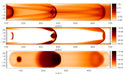
Figure 2.— Top-panel: Logarithmic density map from PLUTO output; Middle: Emissivity in [SII]6716Åin units of erg cm^-3s^-1, logarithmic map; Bottom: Surface brightness map in erg cm^-2arcsec^-2s^-1, logarithmic, angle jet - LoS 45 deg.

After the second step of post-processing, a longitudinal or transversal slit of arbitrary size can be defined on the computed surface brightness map, used to compute synthetic spectra and position-velocity diagrams. The synthetic spectra include the natural and Doppler line broadening, and consist of all emission lines selected for processing, with customizable spectral range and resolution. The resulting position-velocity (PV) diagrams can be directly compared to the ones derived from observations. PV diagrams taken with a slit parallel to the jet axis and stepped across the jet or a slit perpendicular on the jet axis are particularly useful for simulations that include the rotation of the jet. This is expected from models of jet generation, and indications of rotation have been detected in several microjets in recent works (Bacciotti et al., 2002; Woitas et al., 2005; Coffey et al., 2004, 2007).

It is also possible to extract velocity channel maps in custom velocity channels and emission lines, to be compared with observations. These velocity channel maps are of paramount importance in the investigation of jet structure.

3. Results

We discuss the results of the numerical simulations and compare these with observations of emission knots of the three sources, for which high-quality observational data are available in the literature. The jets obtained with the numerical simulations have been projected at an angle of 45 degrees with the line of sight, taking as a reference the case of the RW Aurigae jets.

3.1. Shocked jet emission

In the simulation set $A$, the equilibrium of a cylindrical jet is guaranteed by the toroidal component of the magnetic field vector and the density along the jet remains uniform, thus the first shock propagates in a constant density environment. On the contrary, the second and the third shocks in the array travel in the decreasing density zone following the propagation of the previous shock, ensuring a longer time-span for intense line emission. Indeed, following the evolution of the shocks over time, one can notice the different behaviour of the second shock with respect to the first one, being brighter over a larger distance.

Fig. 3 shows surface brightness maps in three emission lines from [SII], [OI], and [NII] respectively, for a simulation type $A$. In this case the jet variability period is 10 years, the perturbation amplitude 50km/s and the temperature of the jet material 2 500K (Hydrogen mostly neutral before the shock). We can see in this figure the sharp decrease of the brightness after the peak of about four orders of magnitude over a distance of 50AU. This leaves large dark spaces between emission knots, that are not seen in observations. We note that an attempt to alleviate this problem by diminishing the time periodicity of the perturbations that evolve in shock waves, lead to a decrease in the maximum knot brightness, explained by the lower mass flux entering each shock.

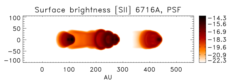
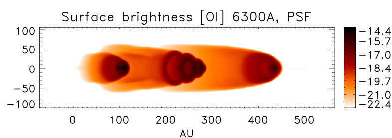
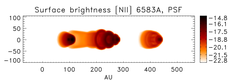
Figure 3.— Simulation in $A$ configuration, no pre-ionization, perturbation amplitude 50km/s, period 10 years, surface brightness in [SII]6716Å(top), [OI]6300Å(middle) and [NII]6583Å, units of erg cm^-2arcsec^-2s^-1, log10 maps.

When an X-ray-induced pre-ionization of the pre-shock medium is considered (about 19% in Hydrogen), Fig. 4, the emission areas behind the shocks are extended compared to previous case, Fig. 3 (in the figures being presented the same moment in the evolution), and the maximum values of the brightness are higher as well. This configuration provides surface brightness maps more similar to observational data, with elongated emission knots because of the higher background ratio of ionized elements in the jet material.

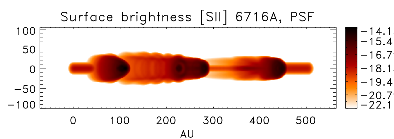
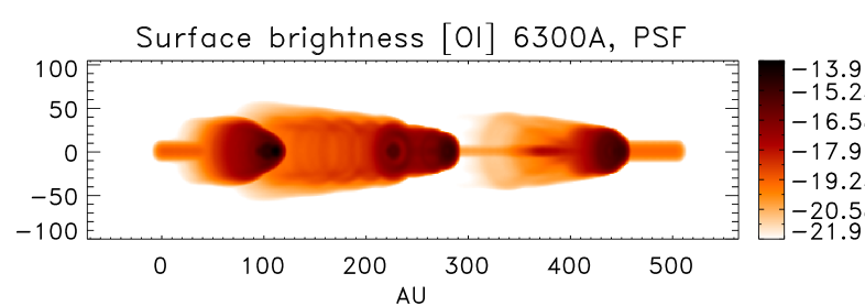
Figure 4.— Simulation in $A$ configuration, pre-ionization 19%, perturbation amplitude 50km/s, period 10 years, surface brightness in [SII]6716Å(top), [OI]6300Å(middle) and [NII]6583Å, units of $erg\cdot cm^{-2}arcsec^{-2}s^{-1}$, log₁₀ maps.

Moreover, the presence of pre-ionization leads to the increase in the peak surface brightness with factors between 2 and 4. This is due to the fact that a pre-existing increased number of free electrons fasten the collisional ionization and excitation, enhancing the total brightness.

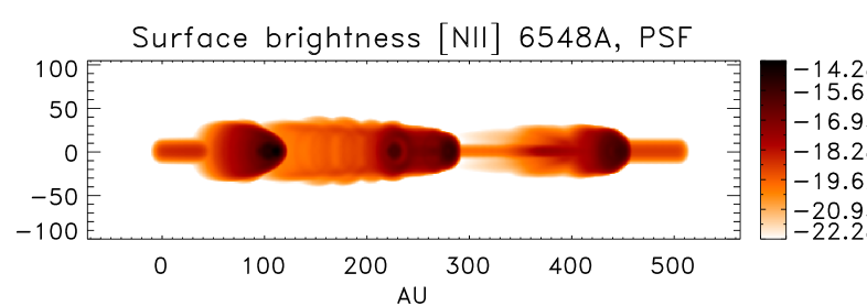
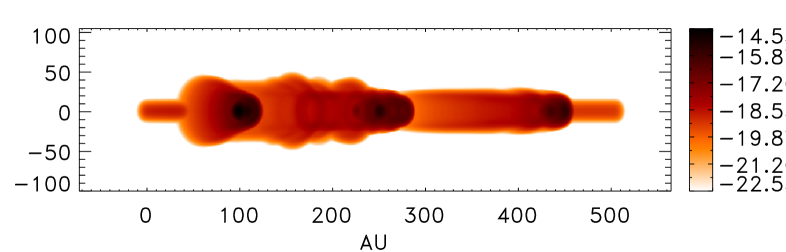
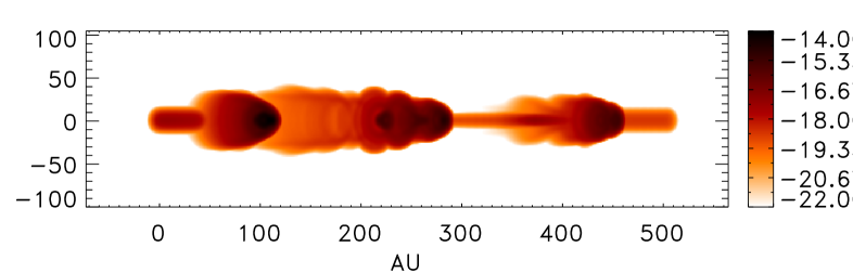
Figure 5.— Surface brightness maps in [NII]6548Å, in four simulation configurations (A, B, C, and D), with pre-ionization and the same set of parameters. Units of erg cm^-2arcsec^-2s^-1, log₁₀ maps.

In Fig. 5 we show a comparison among the simulated surface brightness of the shocked jet in [NII]6548Åfor four different simulation sets (A, B, C, and D from top to bottom panels), including the pre-ionization of the jet material by X-rays. For consistency, the maps are drawn at the same evolutionary stage and the “variable” parameters were set to the same values.

The top panel shows the surface brightness map for a simulation in setup $A$, with rather compact emission knots and low-intensity gaps between them. The $B$ simulation (second panel from top) includes the jet rotation with a maximum velocity of $10km\cdot s^{-1}$, and produces maximum surface brightness lower than in the corresponding $A$ cases, but with a reduced decrease in brightness in the regions between two successive emission peaks. In case $C$ (third panel in Fig. 5), the propagation of the knots is slightly faster with respect to the previous cases, because of the higher density ($5\cdot 10^{4}cm^{-3}$ instead of $10^{4}cm^{-3}$). In addition, the maximum value of the surface brightness is higher than in the otherwise very similar results of case $A$. The results of case $D$ has been obtained setting the jet rotation at $10km\cdot s^{-1}$ and density at $5\cdot 10^{4}cm^{-3}$), and from Fig. 5, bottom panel, we see that the morphology of the line emission is similar to the one of case $B$, but with higher emission intensities due to the increased amount of mass load of the jet.

The purely hydrodynamic case $Ah$ is characterized by a larger lateral expansion, thus both the maximum surface brightness and the length of the high-intensity zone result lower than in the corresponding MHD cases, so it was excluded from the comparison in Fig. 5. The results in the $E$ cases were very similar to the ones obtained in the $D$ setup, thus not displayed.

3.2. Comparison with observations

3.2.1 Observational constraints

We refer to Hubble Space Telescope (STIS instrument) observations of RW Aurigae jets, Melnikov et al. (2009); for DG Tau, Bacciotti et al. (2002) and Lavalley-Fouquet et al. (2000); and for HH30, Hartigan & Morse (2007).

In Fig. 6, we show the observed surface brightness along the jet axis in the three emission doublets of [OI] (6300Åand 6363Å), [NII] (6548Åand 6583Å) and [SII] (6716Åand 6731Å) for the three sources quoted above. Hereafter, where no wavelength is specified, the square brackets notation refers to the sum of both lines of the respective doublet.

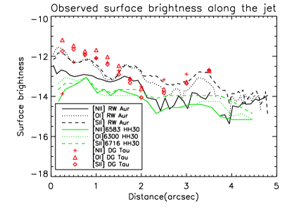
Figure 6.— Surface brightness in along the jets in units of erg cm^-3arcsec^-2s^-1, logarithmic plot on the jet axis from observations of RW Aurigae redshifted jet, DG Tau and HH 30.

One can note the overall higher brightness of the three emission doublets for DG Tau, in agreement with both the higher Doppler velocities measured for this source and the presence of an X-ray emission discovered by the Chandra Observatory (e.g. Schneider & Schmitt (2008)), as possibly indicative stronger shock waves. Working in the approximation of optically-thin plasma, the higher values for the RW Aurigae redshifted jet with respect to HH30 jet, despite the similar flow and shock velocities, may be explained by the higher declination angle of the former with respect to the line of sight and the different toroidal magnetic field strength.

3.2.2 Surface brightness

As discussed in the previous section, the surface brightness variation with distance along the jet differs depending on the case considered. Without including pre-ionization (i.e. with the ionization fraction taken in collisional equilibrium at 2 500K ahead of the shocks), the distribution of surface brightness along the jet (Fig. 7) has variations of many orders of magnitude and lower peak values with respect to the pre-ionized cases (and much lower than observations).

Figure 7.— Surface brightness, doublets of [SII], [OI] and [NII] in units of erg cm^-3arcsec^-2s^-1, logarithmic plot on the jet axis from simulation type $A$, with no pre-ionization.

The rotating jet simulated in configuration $D$ is a good candidate for the comparison with observations, the decrease of brightness between the high-intensity being less pronounced than in the corresponding non-rotating case ($A$) - see Fig. 8.

An important increase in brightness is also important for the comparison with observations – shocks with higher-amplitude perturbations (higher than 50 km s^-1) are not likely for “slow” jets such as HH30 and RW Aur, so the pre-ionization provides a way of enhancing brightness without going with the simulations beyond the most probable parameter range.

Figure 8.— Surface brightness, doublets of [SII], [OI] and [NII] in units of erg cm^-3arcsec^-2s^-1, logarithmic plot on the jet axis from simulation type $D$, with pre-ionization.

The decreasing trend of the peak brightness with the traveled distance from the jet origin is visible both in simulations and observations: at angular distances larger than $2^{\prime\prime}$, the decrease is approximately one order of magnitude (Figs. 6 and 8). This suggests that the knots observed in many jets (e.g. HH 34 and HH 111) at distances of a few tens of arcseconds from the source are likely to arise from other mechanisms, i.e. jets shear-layer instabilities.

3.2.3 Line emission ratios

The line emission ratios are indispensable ingredients in methods for deriving the physical parameters of space plasmas from observations. In the case of stellar jets - the forbidden emission doublets of [SII], [OI] and [NII] between 6 and 7 000Åare used (“BE” technique, Bacciotti et al. (1999)) for this purpose. For this reason the comparison between the observed and simulated line ratios is a powerful method of validation for both the numerical code and the correct interpretation of observational data.

In the previous 1D analyses we considered the emission of a single shock at different times while propagating along the jet, instead we are now taking snapshots at given times of the whole length of the jet and study the behaviour of the line ratios as a function of the longitudinal coordinate. The high numerical resolution achieved thanks to the AMR technique allows us to follow not only the values in the emission peaks, but also their evolution in the post-shock zone as the gas cools. We draw in Fig. 9 the results of the calculations, without pre-ionization, of three line ratios of forbidden lines in comparison with the observed line ratios (symbols) for the first part of the redshifted jet from the RW Aurigae pair. We see that the values of the calculated line ratios approach observations only for short distances after the shocks.

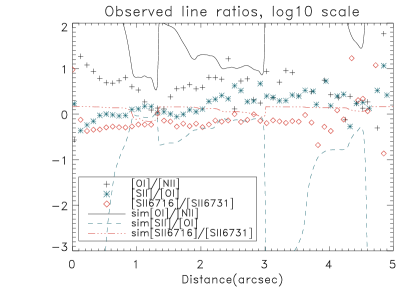
Figure 9.— Line ratios between the three doublets of [SII]6716+6731Å, [OI]6300+6363Åand [NII]6548+6583Å, log10 scale plot on the jet axis from simulation type $A$ without pre-ionization, and observations.

In Figs. 10 and (Fig. 11) we show a simulation from the $A$ and $B$ sets, respectively, with pre-ionization included. In both cases the behaviour of the calculated line ratios is much more consistent with observational data, the variations between knots remaining in the observed ranges.

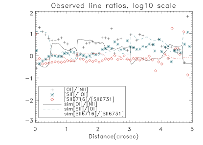
Figure 10.— Line ratios between the three doublets of [SII]6716+6731Å, [OI]6300+6363Åand [NII]6548+6583Å, log10 scale plot on the jet axis from simulation type $A$ with pre-ionization, and observations.

Figure 11.— Line ratios between the three doublets of [SII]6716+6731Å, [OI]6300+6363Åand [NII]6548+6583Å, log10 scale plot on the jet axis from simulation type $B$ with pre-ionization, and observations.

3.3. Position-Velocity diagrams

In order to illustrate the distribution in velocities of the emitting material, the Position-Velocity (PV) diagrams are widely used. A spectrum is generated for each pixel along the spectrograph slit, and the results are plotted in units of surface brightness at a certain wavelength on a Position-Velocity map.

If Fig. 12, the output from the PLUTO post-processing routines is shown. The top panel is a surface brightness map in one of the lines of the [SII] doublet, with the user-defined slit from where the data for the PV-diagram will be taken. The bottom panel displays the resulting PV diagram, in units of surface brightness. The distribution of brightness is concentrated to the right half of the image, corresponding to positive velocities, due to the declination angle between the jet axis and the line of sight. The enhanced emission knots can be clearly seen in the PV diagram, concentrating around radial velocities of 90 km s^-1. The inter-knot jet material is distributed in a range of velocities between -10 and +70 km s^-1.

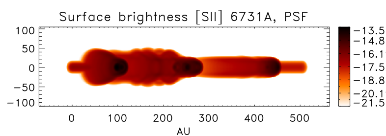
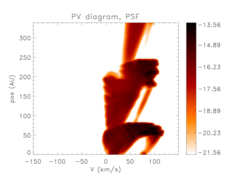
Figure 12.— Surface brightness (top panel) with the defined slit $0^{\prime\prime}.4$ wide (at the distance of Taurus), and position-velocity diagram (bottom) for [SII] 6731Å.

The PV diagrams are a powerful tool in the modern study of the structure of stellar jets, providing more accurate information on the velocity distribution of the emitting material. By the differences in the radial velocity and asymmetries between opposite parts of the jet, their rotation (predicted by models) can be inferred (Coffey et al., 2007). Consequently, as both the spatial and spectral resolutions of observational data increased, these diagrams were geenrated also from the jet models, in order to be compared to the ones derived from observations (Cerqueira et al., 2006; Smith & Rosen, 2007). Arrays of models were devised (Kajdic et al., 2006).

An interesting study underway, where PV diagrams from multiple slits will be employed, focuses on DG-Tau and RW Aurigae, in the search for rotation signatures.

4. Conclusions and summary

Starting from numerical MHD simulations that include ionization network and detailed radiative cooling, we have obtained synthetic emission maps of surface brightness at various wavelengths relevant for observations of HH microjets. The comparison with observations was not limited to surface brightness (along the jet, integrated in velocity), we have also tried to match the observed line ratios for different values of the simulation parameters.

We have shown the crucial role assumed by the pre-existing ionization in the jet medium, prior to the passage of the shock wave, for the line emission properties of the corresponding “knot”. We believe that pre-ionization will be a key ingredient in future work. This relatively high ionization fraction is likely to come from the X-ray photoionization of the atoms at the jet base, being advected away with the flow conserving its value because of the low the recombination rate. The pre-ionization increases the number of free electrons in the gas and speeds up the processes of ionization and excitation at the passage of the shock wave.

Among the simulations performed during this work, the $B$ and $D$ sets, that include a toroidal magnetic field, rotation of the jet and pre-ionization, seem to compare well with observations. Future analyses will address the problem of the contrast between the knots and intra-knots brightness, that remains higher than observed, for performing simulations aiming to reproduce in greater detail the emission features of particular objects, with the goal to constrain the jet physical parameters and better understand the physical mechanisms at work. Moreover, a challenging but potentially insightful investigation will be the 3D case, that could address the shock misalignment.

Appendix A Radial Equilibrium Solution

The equilibrium solution is constructed by considering the radial force balance between pressure, magnetic and centrifugal forces under the assumption $v_{r}=B_{r}=0$. The equilibrium condition is expressed through the steady-state $r$-component of the momentum equation, which reads

$$\frac{dp}{dr}=\frac{\rho v_{\phi}^{2}}{r}-\frac{1}{2}\left[\frac{1}{r^{2}}\frac{d(rB_{\phi})^{2}}{dr}+\frac{dB_{z}^{2}}{dr}\right]\,.$$ (A1)

In the present context, we will ignore the effect of a poloidal field component and simply consider cases with $B_{z}=0$. Density and longitudinal velocity profiles can be chosen to smoothly match their ambient values for $r>R_{j}$ while the azimuthal component of magnetic field is prescribed by

$$B_{\phi}(r)=-\frac{B_{m}}{r}\sqrt{1-\exp\left[-(r/a)^{4}\right]}\,,$$ (A2)

where $a=0.9$ is the magnetization radius and $r_{j}$ is the jet radius. This choice guarantees that at large radii the field becomes essentially force-free whereas close to the axis the electric current $J_{z}\approx-2B_{m}r_{j}/a^{2}$ is approximately constant. A convenient profile for the azimuthal velocity is

$$v_{\phi}(r)=\alpha\frac{rr_{j}}{a^{2}}\sqrt{\frac{2\exp\left[-(r/a)^{4}\right]}{\rho}}\,,$$ (A3)

where the constant $\alpha$ sets the amount of rotation and the relative importance of the centrifugal to the Lorentz force. With these assumptions Eq. (A1) can be integrated giving

$$p(r)=p_{j}+\frac{1}{2}\frac{(\alpha^{2}-B_{m}^{2})\sqrt{\pi}\,\textrm{erf}(r^{2}/a^{2})}{(a/r_{j})^{2}}\,,$$ (A4)

where $p_{j}$ is the jet pressure on the axis. Clearly, when $\alpha>B_{m}$, the gas pressure increases monotonically with $r$ while the opposite is true for $\alpha<B_{m}$. The condition $\alpha=B_{m}$ yields exact balance between rotations and magnetic forces.

The actual value of $\alpha$ can be expressed in terms of the maximum rotation velocity $v_{\phi}^{\max}$ which, in the limit of constant density, becomes

$$\alpha\approx v^{\max}_{\phi}\left(\frac{e}{2}\right)^{1/4}\frac{a}{r_{j}}\sqrt{\rho_{j}}$$ (A5)

Finally, in order to specify the magnetic field strength $B_{m}$, we note that, by assigning the equilibrium ambient temperature $T_{a}=p_{a}\mu_{a}m_{a}/(\rho_{a}k_{B})$ (where $\rho_{a}$ is the ambient density), Eq (A4) may be solved for the magnetic field strength $B_{m}$ giving

$$B_{m}^{2}=\alpha^{2}+\frac{2k_{B}}{\sqrt{\pi}m_{a}}\left(\frac{a}{r_{j}}\right)^{2}\rho_{j}\left(\frac{T_{j}}{\mu_{j}}-\frac{T_{a}}{\eta\mu_{a}}\right)$$ (A6)

where $k_{B}$ is the Boltzmann constant, $m_{a}$ is the atomic mass unit, $\rho_{j}$ is the jet density, $\eta=\rho_{j}/\rho_{a}$ is the jet to ambient density contrast, $\mu_{j}$ and $\mu_{a}$ are the mean molecular weights in the jet and in the ambient medium, respectively. Eq (A6) immediately shows that, for $T_{a}<T_{j}$, the magnetic field has a lower threshold value and its strength always increases with rotation.

References

- Bacciotti et al. (1999) Bacciotti, F., Eislöffel, J. 1999, A&A, 342, 717
- Bacciotti et al. (2002) Bacciotti, F., Ray, T.P., Mundt, R., Eislöffel, J., Solf, J. 2002, ApJ, 576, 222
- Cerqueira et al. (2006) Cerqueira, A.H., Velázquez, P.F., Raga, A.C., Vasconcelos, M.J., de Colle, F. 2006, A&A, 448, 231
- Coffey et al. (2004) Coffey, D., Bacciotti, F., Woitas, J., Ray, T.P., Eislöffel, J. 2004, ApJ, 604, 758
- Coffey et al. (2007) Coffey, D., Bacciotti, F., Ray, T.P., Eislöffel, J., Woitas, J. 2007, ApJ, 663, 350
- Cox & Raymond (1985) Cox, D., & Raymond, J. 1985, ApJ, 298, 651
- Dopita & Sutherland (2003) Dopita, M.A., Sutherland, R.S. 2003, ”Astrophysics of the diffuse universe”, Springer
- Glassgold et al. (1997) Glassgold, A.E., Najita, J., Igea, J. 1997, ApJ, 480, 344
- Güdel (2011a) Güdel, M. 2011a, Bulletin of the American Astronomical Society, Vol. 43
- Güdel et al. (2011b) Güdel, M., Audard, M. Bacciotti, F., & al. 2011b, arXiv:1101.2780v1
- Glassgold et al. (2000) Glassgold, A.E., Feigelson, E.D., Montmerle, T. 2000, Protostars and Planets IV, Tucson: University of Arizona Press (eds Mannings, V., Boss, A.P., Russell, S. S.), p. 429
- Hartigan et al. (1987) Hartigan, P., Hartigan, Raymond, J., Hartmann, L. 1987, ApJ, 316, 323
- Hartigan et al. (1994) Hartigan, P., Morse, J. A., Raymond, J. 1994, ApJ, 436, 125
- Hartigan & Morse (2007) Hartigan, P., & Morse, J. 2007, ApJ, 660, 426
- Kajdic et al. (2006) Kajdic, P., Velázquez, P.F., Raga, A.C. 2006, RMxAA, 42, 217
- Lavalley-Fouquet et al. (2000) Lavalley-Fouquet, C., Cabrit, S., Dougados, C. 2000, A&A, 356, L41
- Massaglia et al. (2005a) Massaglia, S., Mignone, A., Bodo, G. 2005a, A&A, 442, 549
- Matsakos et al. (2009) Matsakos, T., Massaglia, S., Trussoni, E., & al., A&A, 502, 217
- Melnikov et al. (2009) Melnikov, S.Y., Eislöffel, J., Bacciotti, F., Woitas, J., Ray, T.P. 2009, A&A, 506, 763
- Mignone et al. (2007) Mignone, A., Bodo, G., Massaglia, S., Matsakos, T., Tesileanu, O., Zanni, C., Ferrari, A. 2007, ApJS, 170, 228
- Mignone et al. (2009) Mignone, A., Teşileanu, O., Zanni, C. 2009, ”Numerical Modeling of Space Plasma Flows: ASTRONUM-2008”, ASP Conference Series, Vol. 406, 105
- Mignone et al. (2011) Mignone, A., Zanni, C., Tzeferacos, P., et al. 2011, accepted for publication in ApJS
- Preibisch & Neuhäuser (2005) Preibisch, Th.,& Neuhãuser, R. 2005, ApJS, 160, 390
- Raga et al. (2007) Raga, A. C., De Colle, F., Kajdič, P., Esquivel, A., Cantó, J. 2007, A&A, 465, 879
- Rossi et al. (1997) Rossi, P., Bodo, G., Massaglia, S., Ferrari, A. 1997, A&A, 321, 672
- Schneider & Schmitt (2008) Schneider, P.C. & Schmitt, J.H.M.M. 2008, A&A, 488, L13
- Shang et al. (2002) Shang, H., Glassgold, A.E., Shu, F.H., Lizano, S. 2002, ApJ, 564, 853
- Shull & McKee (1979) Shull, J.M., & McKee, C.F. 1979, ApJ, 227, 131
- Shull & van Steenberg (1985) Shull, J.M., & van Steenberg, M.E. 1985, ApJ, 298, 268
- Skinner et al. (2011) Skinner, S. L., Audard, M. & Güdel, M. 2011, ApJ, 737, 19
- Smith & Rosen (2007) Smith, M.D., Rosen, A. 2007, MNRAS, 378, 691
- Takami et al. (2004) Takami, M., Chrysostomou, A., Ray, T.P., & al. 2004, A&A, 416,213
- Teşileanu et al. (2008) Teşileanu, O., Mignone, A., Massaglia, S. 2008, A&A, 488, 429
- Teşileanu et al. (2009a) Teşileanu, O., Massaglia, S., Mignone, A., Bodo, G., Bacciotti, F. 2009a, A&A, 507, 581
- Teşileanu et al. (2009b) Teşileanu, O., Mignone, A., Massaglia, S. 2009b, Procs. ”Protostellar Jets in Context”, T.P. Ray, K. Tsinganos & M. Stute eds., Astrophysics and Space Science Proceedings Series, Springer, p. 447
- Tzeferacos et al. (2009) Tzeferacos, P., Ferrari, A., Mignone, A., & al. 2009, MNRAS, 400, 820
- Verner & Yakovlev (1995) Verner, D.A., Yakovlev, D.G. 1995, A&AS, 109, 125
- Woitas et al. (2005) Woitas, J., Bacciotti, F., Ray, T.P., Marconi, A., Coffey, D., Eislöffel, J. 2005, A&A, 432, 149
- Zanni et al. (2007) Zanni, C., Ferrari, A., Rosner, R., Bodo, G., Massaglia, S. 2007, A&A, 469, 811