Cosmological expansion and local systems: a Lemaître-Tolman-Bondi model

Abstract

We propose a Lemaître-Tolman-Bondi system mimicking a two-body system to address the problem of the cosmological expansion versus local dynamics. This system is strongly bound but participates in the cosmic expansion and is exactly comoving with the cosmic substratum.

1 Introduction

The problem of the influence of the cosmological expansion on local gravitationally bound systems was apparently first raised by McVittie in 1933 McVittie33 , studied by Einstein and Straus EinsteinStraus45 ; EinsteinStraus46 , and then debated in dozens of papers stretching to our days (see the recent review by Carrera and Giulini CarreraGiulini10 ).

The problem is the following: for a local system such as a planetary system, a binary stellar system, or a galaxy in the expanding universe, does the cosmological expansion affect the local dynamics of this system and, if so, in which way and, numerically, to what extent? Many authors support the view that the cosmic expansion affects only systems larger than a certain spatial scale and there is no effect below that scale. However, it has not been possible to assess what this scale is, or what determines it CarreraGiulini10 ; FaraoniJacques07 . It seems that, assuming in principle the Friedmann-Lemaître-Robertson-Walker (FLRW) metric to be valid down to small scales (possibly with some modifications that describe local inhomogeneities McVittie33 ; Lemaitre ; Tolman ; Bondi ), all systems are subject to the effect of the cosmic expansion, although this effect is numerically negligible for small systems and stronger for larger and larger objects, up to the scale of galaxy clusters for which it becomes significant. Even atoms have been considered as local systems Bonnor ; Price , and a connection with the well known anomaly observed in the Pioneer satellites has been proposed Pioneer , although there is no foundation for attributing the Pioneer anomaly to the cosmic expansion CarreraGiulini10 . Following the introduction of the dark energy concept to explain the present acceleration of the universe discovered with type Ia supernovae SN and the realization that this dark energy could potentially take the form of phantom energy leading to a Big Rip singularity at a finite future BigRip , the effect of the cosmological expansion on local systems as the Big Rip is approached seems to go unquestioned even though the persistence of cosmic effects on local systems in an adiabatic approximation in which the Hubble scale is much larger than the typical scales for local dynamics is often denied (see FaraoniJacques07 for details).

Two lines of approach to the problem of cosmological expansion versus local dynamics have been followed. The most common approach studies a Newtonian gravitationally bound system, such as a binary stellar system embedded in an expanding FLRW universe and computes the effect of the cosmic expansion as a perturbation of the local dynamics. The result for a particle of polar coordinates $\left(r,\varphi\right)$ and angular momentum $L$ in the field of a mass $M$ embedded in a FLRW universe with scale factor $a(t)$ is given by the equations of motion CooperstockFaraoniVollick98 ; FaraoniJacques07 ; CarreraGiulini10 :

$$\ddot{r} = -\frac{M}{r^{2}}+\frac{L^{2}}{r^{2}}+\frac{\ddot{a}}{a}\,r\,,$$ (1)

$$\dot{\varphi} = \frac{L}{r^{2}}\,.$$ (2)

The second approach, originally pursued with the McVittie solution McVittie33 and the Einstein-Straus vacuole EinsteinStraus45 ; EinsteinStraus46 used analytical solutions of the Einstein equations to describe a local (spherically symmetric) inhomogeneity embedded in a FLRW universe (see Krasinski for a review of inhomogeneous cosmological models). The Lemaître-Tolman-Bondi (LTB) class of solutions (e.g., Ivanareview ) describes a spherical inhomogeneity embedded in a dust-dominated (pressureless) FLRW universe. Here we propose, in the LTB class of solutions, a particularly clear example of a local system composed of two spherical shells with density merging smoothly with the cosmic substratum, which is embedded in a FLRW universe. These shells have zero angular momentum and are kept at finite distance from each other by the cosmic expansion. Clearly, the latter has a non-negligible effect on the local dynamics of this system, independent of the strength of the local interaction. In fact, the effect of the cosmological expansion on the local two-shell system persists even in the limit in which the ratio between local and cosmological densities is arbitrarily large. For simplicity, we consider a spatially flat FLRW background and we follow the notations of Ref. Wald . The metric signature is $-+++$ and units are used in which the speed of light in vacuo $c$ and the gravitational constant $G$ assume the value unity.

2 An exact two body system in a cosmological background

The LTB line element is Lemaitre ; Tolman ; Bondi

$$ds^{2}\,=\,-dt^{2}+\left[R^{\prime}(t,r)\right]^{2}dr^{2}+R^{2}\left(t,r\right)\,d\Omega^{2}\ ,$$ (3)

where $r$ is a comoving radius, $d\Omega^{2}=d\vartheta^{2}+\sin^{2}\vartheta\,d\varphi^{2}$ is the metric on the unit $2$-sphere,

$$R\left(t,r\right)=\left(r^{3/2}+\frac{3}{2}\,\sqrt{m_{e}(r)}\,\,t\right)^{2/3}$$ (4)

is an areal radius,

$$m_{e}(r)=4\pi\int\limits_{0}^{r}dr^{\prime}\,r^{\prime 2}\rho_{0}(r^{\prime})\,,$$ (5)

is called the “Euclidean mass”, and $\rho_{0}(r)$ is the energy density on an initial hypersurface. The areal radius (4) is obtained as solution of the classical Bondi equation Lemaitre ; Tolman ; Bondi ; Ivanareview

$$\dot{R}^{2}(t,r)\,=\,\frac{m_{e}(r)}{R(t,r)}\ .$$ (6)

A prime and a dot denote differentiation with respect to $r$ and $t$, respectively.

Let us consider, at the initial time, a density function that has two equal peaks located at $r_{1}$ and $r_{2}$ (with $r_{2}>r_{1}$)

$$\rho_{0}(r)=\rho_{c}+\rho_{*}\,\,\left[\frac{1}{\left(r-r_{1}\right)^{2}+a^{2}}+\frac{1}{\left(r-r_{2}\right)^{2}+a^{2}}\right]\ ,$$ (7)

where $\rho_{c}$ is a positive constant denoting the density of a cosmological background far away from the density peaks, i.e., $\rho_{0}(r)\,\approx\,\rho_{c}$ as $r\rightarrow+\infty$, and $\rho_{*}$ is proportional to the peak density with $\rho_{*}/a^{2}>\rho_{c}$.

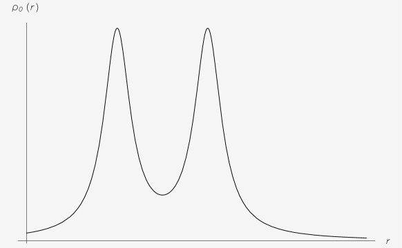
Figure 1: The initial density $\rho_{0}(r)$ for the parameters choice $\rho_{c}=\,1,\rho_{*}=2,a^{2}=2,r_{1}=8$, and $r_{2}=16$ (in arbitrary units).

With the choice (7) for the initial density $\rho_{0}(r)$, the Euclidean mass can be calculated explicitly as (see Figs. 1, 2)

$$m_{e}(r) = \frac{4\pi}{3}\rho_{c}r^{3}+8\pi\rho_{*}r$$ (8)

$$+ 4\pi\rho_{*}\left\{\frac{\left(r_{1}^{2}-a^{2}\right)}{a}\,\,\left[\tan^{-1}\left(\frac{r-r_{1}}{a}\right)+\tan^{-1}\left(\frac{r_{1}}{a}\right)\right]+\right.$$

$$+ \left.r_{1}\log\left[\frac{\left(r-r_{1}\right)^{2}+a^{2}}{r_{1}^{2}+a^{2}}\right]\right\}+$$

$$+ 4\pi\rho_{*}\left\{\frac{\left(r_{2}^{2}-a^{2}\right)}{a}\,\,\left[\tan^{-1}\left(\frac{r-r_{2}}{a}\right)+\tan^{-1}\left(\frac{r_{2}}{a}\right)\right]\right.$$

$$+ \left.r_{2}\log\left[\frac{\left(r-r_{2}\right)^{2}+a^{2}}{r_{2}^{2}+a^{2}}\right]\right\}\ .$$

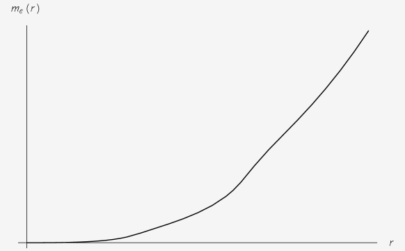
Figure 2: The Euclidean mass $m_{e}(r)$.

This Euclidean mass is related to the Misner-Sharp-Hernandez mass and to the Hawking-Hayward quasi-local mass. The Misner-Sharp-Hernandez mass $M_{MSH}$ is defined, for a spherically symmetric metric, by MisnerSharp64 ; HernandezMisner66

$$1-\frac{2\,M_{MSH}}{R}=\nabla^{\mu}R\nabla_{\mu}R=1-R_{t}^{2}=1-\frac{\,m_{e}\left(r\right)}{R}$$ (9)

from which it follows that

$$M_{MSH}=\frac{\,m_{e}\left(r\right)}{2}=2\pi\int\limits_{0}^{r}ds\,\rho_{0}(s)s^{2}\,.$$ (10)

The first equality is independent of the particular form of the initial density distribution $\rho_{0}(r)$. Further, with spherical symmetry, the Misner-Sharp-Hernandez mass coincides with the Hawking-Hayward quasi-local mass Hawking68 ; Hayward86 .

With a slight abuse of terminology, the two density peaks at $r_{1}$ and $r_{2}$ will be called “shells”. In actual fact, they are not sharp shells, but continuous distributions of matter more or less peaked according to the value of the parameter $a$ appearing in (7), and with maximum density controlled by the parameter $\rho_{*}$. This two-“shell” system mimicks the binary system of test particles chosen in many works to assess the effect of the cosmic expansion on local systems CarreraGiulini10 , but with two importance differences. First, there is zero angular momentum, no direction is preferred, and spherical symmetry holds because instead of a single test particle orbiting around a centre of force and subject to the cosmic expansion as a perturbation of this motion, we now have a spherical “shell” surrounding a smaller “shell” acting as a centre of force. Second, there is no test particle here: the dust with density $\rho$ gravitates and curves spacetime. Instead of treating the cosmic expansion as a small perturbation of a weakly gravitating system, we have an exact solution describing at once the spacetime and the two-shells matter distribution, which merge smoothly with the cosmological background, and this is the virtue of our LTB example. No approximations are made and no adiabatic expansion in term of local and Hubble time scales is necessary. The element of proper radial distance is (setting $dt$, $d\vartheta$, and $d\varphi$ equal to zero) $dl\,=\,R^{\prime}dr$. Using the fact that $dR\,=\,R_{t}dt+R^{\prime}dr$, we have $dl\,=\,dR$ for $dt\,=\,0$. Therefore, the proper radial distance between the two density peaks on a constant time slice of the LTB spacetime is

$$\emph{l}_{12}(t) = R_{2}-R_{1}\equiv R(t,\,r_{2})-R(t,\,r_{1})=$$ (11)

$$= \left(\,r_{2}^{3/2}+\frac{3}{2}\sqrt{m_{e}\left(r_{2}\right)}\,t\right)^{2/3}-\left(\,r_{1}^{3/2}+\frac{3}{2}\sqrt{m_{e}\left(r_{1}\right)}\,t\right)^{2/3}\,.$$

This quantity can be regarded as the size of the two-shell system and corresponds, roughly speaking, to the radius of the binary system considered in previous works. However, $l_{12}$ is now a proper distance, not a coordinate distance (the use of misleading coordinate systems has led to coordinate-based statements and has marred many investigations of this problem). At the time $t\,=\,0$ this proper radial distance coincides with the comoving coordinate distance $\left(r_{2}-r_{1}\right)$, but it departs from it for $t>0$. A plot of $l_{12}$ is given in fig. 3.

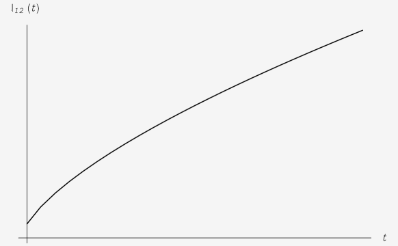
Figure 3: The proper distance ${l}_{12}(t)$ as a function of the comoving time. At $t=0$, $l_{12}$ coincides with the comoving coordinate distance $r_{2}-r_{1}$.

At large times $t\rightarrow+\infty$, it is

$$\l_{12}(t)\approx\left(\frac{3}{2}\right)^{2/3}\left[\left(\sqrt{m_{e}\left(r_{2}\right)}\right)^{2/3}-\left(\sqrt{m_{e}\left(r_{1}\right)}\right)^{2/3}\right]t^{2/3}\,,$$ (12)

i.e., the size $l_{12}$ of the two-shell system is comoving and scales like the scale factor $a(t)\sim t^{2/3}$ of a dust-dominated FLRW universe, to which LTB spacetimes reduce for large $r$. This result matches the one for the Einstein-Straus vacuole EinsteinStraus45 ; EinsteinStraus46 ; Schucking54 in which a spherical central inhomogeneity is surrounded by a spherical vacuum, which is matched to a dust-dominated FLRW space. The proper radius of this matching surface is perfectly comoving CarreraGiulini10 .

We can now discuss the initial conditions in our model. The initial radial separation $l_{12}(0)=R(0,r_{2})-R(0,r_{1})=r_{2}-r_{1}$ between the two “shells” can be taken arbitrarily. Following equation (6), their relative (radial) velocity at time $t$ is

$$\dot{l}_{12}(t)=\dot{R}\left(t,r_{2}\right)-\dot{R}\left(t,r_{1}\right)=\pm\Bigg{(}\sqrt{\frac{m_{e}(r_{2})}{R(t,r_{2})}}-\sqrt{\frac{m_{e}(r_{1})}{R(t,r_{1})}}\Bigg{)}\,.$$ (13)

At the initial time $t=0$, it is

$$\dot{l}_{12}(0)=\pm\Bigg{(}\sqrt{\frac{m_{e}(r_{2})}{r_{2}}}-\sqrt{\frac{m_{e}(r_{1})}{r_{1}}}\Bigg{)}\,.$$ (14)

The functions $\sqrt{m_{e}(r)/r}$ and $-\sqrt{m_{e}(r)/r}$ are plotted in fig. 4. They are, respectively, always increasing and always decreasing, therefore the sign of the initial relative velocity $\dot{l}_{12}(0)$ of the two “shells” is conserved. Assuming that the relative initial velocity of the “shells” is not sufficiently large that the shells collide and cause shell singularities (then the formalism outlined above remains valid), the relative velocity of the “shells” $\dot{l}_{12}$ given by eq. (13) tends to zero because $R(t,r)\propto t^{2/3}$. The “shells” then become comoving.

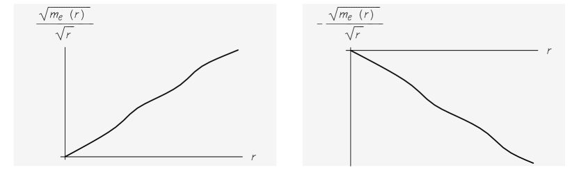
Figure 4: The functions $\sqrt{m_{e}(r)/r}$ and $-\sqrt{m_{e}(r)/r}$ for the choice (7) of the initial density and the same parameter values of fig. 1.

3 Discussion

Generally speaking, the Hubble flow washes out the effects of a local overdensity; this fact is well known in FLRW universes and it occurs also in LTB spacetimes. The following argument is a bit naive but nevertheless carries some weight: consider a function $f(r)$ and its radial gradient $\frac{\partial f}{\partial R}$ with respect to the physical (areal) radius $R$ (the only spatial gradient allowed in the presence of spherical symmetry). It is straightforward to see that

$$\frac{\partial f}{\partial R}=\frac{df/dr}{\partial R/\partial r}=\frac{\left[\sqrt{m_{e}(r)}\left(r^{3/2}+\frac{3}{2}\,\sqrt{m_{e}(r)}\,t\right)^{1/3}\right]}{\sqrt{rm_{e}(r)}+2\pi r^{2}\rho_{0}(r)t}\,\frac{df}{dr}$$ (15)

and, therefore, $\partial f/\partial R\longrightarrow 0$ as $t\rightarrow+\infty$. The evolution of our LTB model is in agreement with this general feature.

In our LTB model, in which the density contrast is smoothed out by the cosmic expansion, the energy density on an initial hypersurface can be chosen at will and the expression (7) describes two local concentrations of matter (“shells”) merging smoothly with the cosmological background. These two “shells” play a role analogous to that of a binary system composed of two test particles embedded in a FLRW background universe so often considered in studies of the effects of the cosmological expansion on local systems. We have chosen the peaks of the initial density distribution to be of equal height for simplicity but this assumption is not necessary: the ratio of their heights can be chosen at will, in the same way that the masses of a binary system subject to the effect of the cosmological expansion can be chosen in any ratio. The LTB example that we presented has two clear advantages over the binary: first, it is a fully gravitating configuration, not a system of test particles and one does not need to resort to approximations in order to embed this system into a cosmological background. This is an exact solution of the Einstein equations. Second, due to the non linearity of general relativity, when one wants to consider cosmic expansion versus local dynamics, it is a priori difficult or impossible to split a solution into a background plus an inhomogeneity (apart from perturbative regimes, which are nevertheless subject to the notorious gauge-dependence problems and require the use of gauge-invariant formalisms): this is exactly what the LTB metric (or the McVittie metric McVittie33 ; FaraoniJacques07 ; CarreraGiulini10 ) does for us.

It is reasonable to regard the proper radial distance $l_{12}\,=\,R_{2}-R_{1}$ between the two “shells” as the physical size of the local system. This quantity depends on time and it is straightforward to see that this distance is comoving with the cosmic dust of the FLRW background. In the LTB example proposed, the local system is affected by the cosmic expansion, regardless of its spatial size. One can take the limit $\rho_{*}\rightarrow 0$ in which the system becomes a test fluid, or the opposite limit $\rho_{*}/a^{2}\gg\rho_{c}$ in which the local system is strongly gravitating. The initial distance $R_{2}-R_{1}\,=\,r_{2}-r_{1}$ between the two density peaks can be adjusted at will in comparison with the Hubble radius $H^{-1}$ of the FLRW background. Any way these parameters are varied, the result is always the same: the local system is stretched by the cosmological expansion and participates in it. This fact shows that, assuming the FLRW metric to describe the universe down to small scales, it is not true that systems below a certain spatial scale are unaffected while only larger ones partake into the expansion, as suggested by many authors (see FaraoniJacques07 ; CarreraGiulini10 for references). By choosing the LTB metric as an example, we were bound to find this result; indeed, it is built into the LTB metric itself. One may, therefore, question the validity of our argument. The point is that a solution with these properties does exist, it is a perfectly legitimate example, and one of the rare exact solutions of the Einstein equations in which a clear answer to the puzzle of cosmic expansion versus local dynamics can be obtained. The answer matches the results obtained with the Einstein-Straus vacuole EinsteinStraus45 ; EinsteinStraus46 ; Schucking54 ; CarreraGiulini10 , McVittie Nolan ; CarreraGiulini10 , generalized McVittie solutions FaraoniJacques07 , and LTB black holes Gaoetal2011 . From the physical point of view, a relevant issue is whether the two-shell system is stable, but this question can also be posed for any LTB metric.

One potential problem with the LTB model proposed here consists of the possible presence of shell-crossing singularities in the $t<0$ region of this spacetime. Although these singularities are not mandatory in LTB models (conditions for their avoidance are given in Ref. HellabyLake ), they are to be expected in general. The prevailing opinion about shell-crossing singularities is that they are an artifact of the dust equation of state chosen and should disappear when, more realistically, some pressure is introduced (see, e.g., Ref. MTW ) although, to be honest, we do not know of a rigorous mathematical proof of this statement to date. Overall, we regard the possibility of shell-crossing singularities as a non-essential feature of LTB models and we choose to focus on the region of LTB spacetime which is free of these singularities.

Finally, we could make the two shells of our model infinitely thin and, in this case, they would have to be matched to their surroundings by using the Darmois-Israel junction conditions junction . However, this construction is not necessary and by continuity of the property presented here, one expects that a system composed of two zero-thickness shells will also be comoving. The case of a single shell matched through the junction conditions to an expanding FLRW universe, and hosting a wormhole, was considered in Refs. FaraoniIsrael05 ; BochicchioFaraoni10 with the result that, even if the shell initially has a non-vanishing velocity relative to the cosmic substratum, it eventually becomes comoving with it.The answer to the question of cosmic expansion versus local dynamics seems to be that expansion wins and local systems go with the (Hubble) flow.

- (1) McVittie, G.C., Mon. Not. R. Astr. Soc. 93, 325 (1933).
- (2) Einstein, A. and Straus, E.G., Rev. Mod. Phys. 17, 10 (1945).
- (3) Einstein, A. and Straus,E.G., Rev. Mod. Phys. 18, 148 (1946).
- (4) Carrera, M. and Giulini, D., Rev. Mod. Phys. 82, 169 (2010).
- (5) Faraoni, V. and Jacques, A., Phys. Rev. D 76, 063510 (2007).
- (6) Lemaître, G., Ann. Soc. Sci. Brussels A 53, 51 (1933), reprinted in Gen. Relat. Gravit. 29, 641 (1997).
- (7) Tolman, R.C., Proc. Nat. Acad. Sci. U.S.A. 20, 169 (1934).
- (8) Bondi, H., Mon. Not. R. Astron. Soc. 107, 410 (1947).
- (9) Bochicchio, I., Francaviglia, M., and Laserra, E., Int. J. Geom. Meth. Mod. Phys. 6, 595 (2009).
- (10) Bonnor, W.B., Class. Quantum Grav. 16, 1313 (1999).
- (11) Price, R.H., Romano J.D., arXiv:gr-qc/0508052 (2012).
- (12) Mizony, M. and Lachièze-Rey, M., Astron. Astrophys. 434, 45 (2005); Izzo, D. and Rathke, A., J. Spacecraft and Rockets 43, 806 (2006); Oliveira, F.J., gr-qc/0610029 (1998); Lachièze-Rey, M., Class. Quantum Grav. 24, 2735 (2007); Rosales, J. and Sanchez-Gomez, J., gr-qc/9810085 (1998); Lammerzhal, C. and Preuss, O., Int. J. Mod. Phys. D 16, 2165 (2007); Turyshev, S.G. and Williams, J.G., Int.J.Mod.PhycsD 16:2165-2179 (2007); Fahr, H.-J. and Siewert, M., gr-qc/0610034 (2006); Williams, J.G., Turyshev, S.G., and Boggs, D.H., Phys. Rev. Lett. 98, 059002 (2007); Dumin, Y.V. Phys. Rev. Lett. 98, 059001 (2007).
- (13) Riess, A.G. et al., Astron. J. 116, 1009 (1998); Astron. J. 118, 2668 (1999); Astrophys. J. 560, 49 (2001); Astrophys. J. 607, 665 (2004); Perlmutter, S. et al., Nature 391, 51 (1998); Astrophys. J. 517, 565 (1999); Tonry, J.L. et al., Astrophys. J. 594, 1 (2003); Knop, R. et al., Astrophys. J. 598, 102 (2003); Barris, B. et al., Astrophys. J. 602, 571 (2004).
- (14) Caldwell, R.R., Kamionkowski, M. and Weinberg, N.N., Phys. Rev. Lett. 91, 071301 (2003); Carroll, S.M., Hoffman, M., and Trodden, M., Phys. Rev. D 68, 023509 (2004).
- (15) Cooperstock, F.I., Faraoni, V., and Vollick, D.N., Astrophys. J. 503, 61 (1998).
- (16) Krasinski, A., Inhomogeneous Cosmological Models (Cambridge University Press, Cambridge, 1998).
- (17) Wald, R.M., General Relativity (Chicago University Press, Chicago, 1984).
- (18) Misner, C.W. and Sharp, D.H., Phys. Rev. 136, 571 (1964).
- (19) Hernandez, J.C. and Misner, C.W., Astrophys. J. 143, 452 (1966).
- (20) Hawking, S.W., J. Math. Phys. 9, 589 (1968).
- (21) Hayward, S.A., Phys. Rev. D 49, 831 (1994).
- (22) Schücking, E., Z. Phys. 1837, 595 (1954).
- (23) Nolan, B.C., Class. Quantum Grav. 16, 1227 (1999); Phys. Rev. D 58, 064006 (1998); Lake, K. and Abdelqader, M., Phys. Rev. D 84, 044045 (2011).
- (24) Gao, C., Chen, X., Shen, Y.-G., and Faraoni, V., Phys. Rev. D 84, 104047 (2011).
- (25) Lanczos, C., Ann. Phys. (Leipzig) 24, 518 (1924); Israel, W., Nuovo Cimento 44B, 1 (1966); 48B, 463(E) (1967).
- (26) Faraoni, V. and Israel, W., Phys. Rev. D 71, 064017 (2005).
- (27) Bochicchio, I. and Faraoni, V., Phys. Rev. D 82, 044040 (2010).
- (28) Hellaby, C. and Lake, K., Astrophys. J. 290, 381 (1985).
- (29) Misner, C.W., Thorne, K.S., and Wheeler, J.A., Gravitation, (Freeman, new York, 1973), p. 859.