Bootstrap inference for network construction with an application to a breast cancer microarray study

Abstract

Gaussian Graphical Models (GGMs) have been used to construct genetic regulatory networks where regularization techniques are widely used since the network inference usually falls into a high–dimension–low–sample–size scenario. Yet, finding the right amount of regularization can be challenging, especially in an unsupervised setting where traditional methods such as BIC or cross-validation often do not work well. In this paper, we propose a new method—Bootstrap Inference for Network COnstruction (BINCO)—to infer networks by directly controlling the false discovery rates (FDRs) of the selected edges. This method fits a mixture model for the distribution of edge selection frequencies to estimate the FDRs, where the selection frequencies are calculated via model aggregation. This method is applicable to a wide range of applications beyond network construction. When we applied our proposed method to building a gene regulatory network with microarray expression breast cancer data, we were able to identify high-confidence edges and well-connected hub genes that could potentially play important roles in understanding the underlying biological processes of breast cancer.

T1Supported by NIH Grants R01GM082802 (SL, JP, PW), P01CA53996 (LH, PW), R01AG014358 (SL, LH), P50CA138293 (LH, PW), U24CA086368 (PW), NSF Grant DBI-08-20854 (JP) and DMS-10-07583 (JP).

, , and

1 Introduction

The emergence of high-throughput technologies hasmade it feasible to measure molecular signatures of thousands of genes/proteins simultaneously. This provides scientists an opportunity to study the global genetic regulatory networks, shedding light on the functional interconnections among the regulatory genes, and leading to a better understanding of underlying biological processes. In this paper, we propose a network building procedure for learning genetic regulatory networks. Our work is motivated by an expression study of breast cancer (BC) that aims to infer the network structure based on 414 BC tumor samples [Loi et al. (2007)]. The proposed method enables us to detect high-confidence edges and well-connected hub genes that include both those previously implicated in BC and novel ones that may warrant further follow-up.

In practice, dependency structures of molecular activities such as correlation matrix and partial correlation matrix have been used to infer regulatory networks [Pollack et al. (2002), Kim et al. (2006), Varambally et al. (2005), Nie, Wu and Zhang (2006)]. Such dependency structures are often represented by graphical models in which nodes of a graph represent biological components such as genes or proteins, and the edges represent their interactions. These interactions may be indirect (e.g., two genes are co-regulated by a third gene) or direct (e.g., one gene is regulated by another gene). For the latter case, Gaussian Graphical Models (GGMs), which represent dependencies between pairs of nodes conditioning on the remaining of nodes, are often used.

For the data obtained from high-throughput technologies, the number of nodes is typically much larger than the number of samples, which is where the classical GGM theory [Whittaker (1990)] generally fails [Friedman (1989), Schaäfer and Strimmer (2005)]. This large-$p$-small-$n$ scenario is usually addressed by assuming that the conditional dependency structure is sparse [Dobra et al. (2004), Li and Gui (2006), Meinshausen and Buühlmann (2006), Yuan and Lin (2007), Friedman, Hastie and Tibshirani (2008), Rothman et al. (2008), Peng et al. (2009)]. However, like many high-dimensional regularization problems, finding the appropriate level of sparsity remains a challenge. This is particularly true for network structure learning, since the problem is unsupervised in nature. Traditional methods, such as Bayes information criteria [Schwarz (1978)] and cross-validation, aim to find a model that minimizes prediction error or maximizes a targeted likelihood function. They tend to include many irrelevant features [e.g., Efron (2004b), Efron et al. (2004), Meinshausen and Bühlmann (2006) and Peng et al. (2010)], and thus are not appropriate for learning the interaction structures.

Choosing the amount of regularization by directly controlling the false positive level would be ideal for structure learning. Recently, a few model aggregation methods have been proposed, and some of them provide certain control of false positives. For example, Bach (2008) proposed Bolasso, which chooses variables that are selected by all the lasso models [Tibshirani (1996)] built on bootstrapped data sets. In the context of network reconstruction, Peng et al. (2010) proposed choosing edges that are consistently selected across at least half of the cross-validation folds. More recently, Meinshausen and Bühlmann (2010) proposed the stability selection procedure to choose variables with selection frequencies exceeding a threshold. Under suitable conditions, they derived an upper bound for the expected number of false positives. In the same paper they also proposed the randomized lasso penalty, which aggregates models from perturbing the regularization parameters. Combined with stability selection, randomized lasso achieves model selection consistency without requiring the irrepresentable condition [Zhao and Yu (2006)] that is necessary for lasso to achieve model selection consistency. In another work, Wang et al. (2011) proposed a modified lasso regression—random lasso—by aggregating models based on bootstrap samples and random subsets of variables. All these works have greatly advanced research in model selection in the high-dimensional regime. However, none of these methods provide direct estimation and control of the false discovery rate (FDR).

In this paper, we address the problem of finding the right amount of regularization in the context of high-dimension GGMs learning. In a spirit similar to the aforementioned methods, we first obtain selection frequencies from a collection of models built by perturbing both the data and the regularization parameters. We then model these selection frequencies by a mixture distribution to yield an estimate of FDR on the selected edges, which is then used to determine the cut-off threshold for the selection frequencies. This framework is rather general, as it only depends on the empirical distribution of the selection frequencies. Thus, it can be applied to a wide range of problems beyond GGMs.

The rest of this paper is organized as follows. In Section 2 we describe in detail the proposed method. In Section 3 an extensive simulation study is conducted to compare the method with the stability selection procedure and then evaluate its performance under different settings. In Section 4 the method is illustrated by building a genetic interaction network based on microarray expression data from a BC study. The paper is concluded with some discussion in Section 5.

2 Method

2.1 Gaussian graphical models

In a Gaussian Graphical Model (GGM) network construction is defined by the conditional dependence relationships among the random variables. Let $Y=(Y_{1},\ldots,Y_{p})$ denote a $p$-dimension random vector following a multivariate normal distribution $N(0,\Sigma)$, where $\Sigma$ is a $p\times p$ positive definite matrix. The conditional dependence structure among $Y$ is represented by an undirected graph $G=(U,E)$ with vertices $U=\{1,2,\ldots,p\}$ representing $Y_{1},\ldots,Y_{p}$ and the edge set $E$ defined as

$$E=\bigl{\{}(i,j)\dvtx Y_{i}\mbox{ and }Y_{j}\mbox{ are dependent given }Y_{-\{i,j\}},1\leq i,j\leq p\bigr{\}},$$

where $Y_{-\{i,j\}}\equiv\{Y_{k}\dvtx k\not=i,j,1\leq k\leq p\}$. The goal of network construction is to identify the edge set $E$. Under the normality assumption, the conditional independence between $Y_{i}$ and $Y_{j}$ is equivalent to the partial correlation $\rho_{ij}$ between $Y_{i}$ and $Y_{j}$ given $Y_{-\{i,j\}}$ being zero. It is also equivalent to the $(i,j)$ entry of the concentration matrix ($\Sigma^{-1}$) being zero, that is, $\sigma_{ij}\equiv(\Sigma^{-1})_{ij}=0$ [Dempster (1972), Cox and Wermuth (1996)], since $\rho_{ij}=-\frac{\sigma_{ij}}{\sqrt{\sigma_{ii}\sigma_{jj}}}$.

There are two main types of approaches to fitting a GGM. One is the maximum-likelihood-based approach, which estimates the concentration matrix directly. The other is the regression-based approach, which fits the GGM through identifying nonzero regression coefficients of the following regression:

$$Y_{i}=\sum_{j\not=i}\beta_{ij}Y_{j}+\varepsilon_{i},\qquad 1\leq i\leq p,$$

where $\varepsilon_{i}$ is uncorrelated with $Y_{-i}=\{Y_{k},k\not=i,1\leq k\leq p\}$. The nonzero $\beta_{ij}$’s in the above regression setting correspond to nonzero entries in the concentration matrix since it can be shown that $\beta_{ij}=-\sigma_{ij}/\sigma_{ii}=\rho_{ij}\sqrt{\sigma_{jj}/\sigma_{ii}}$. In both approaches, there are $O(p^{2})$ parameters to estimate, which requires proper regularization on the model if $p$ is larger than the sample size $n$. This can be achieved by making a sparsity assumption on the network structure, that is, assuming that most pairs of variables are conditionally independent given all other variables. Such an assumption is reasonable for many real life networks, including genetic regulatory networks [Gardner et al. (2003), Jeong et al. (2011), Tegner et al. (2003)]. Methods have been developed along these lines by using $L_{1}$ regularization. For example, Yuan and Lin (2007) proposed a sparse estimator of the concentration matrix via maximizing the $L_{1}$ penalized log-likelihood. Efficient algorithms were subsequently developed to fit this model with high-dimensional data [Friedman, Hastie and Tibshirani (2008), Rothman et al. (2008)]. For regression-based approaches, Meinshausen and Bühlmann (2006) considered the neighborhood selection estimator by minimizing $p$ individual loss functions

$$L^{(i)}(\beta,Y)=\frac{1}{2}\biggl{\|}Y_{i}-\sum_{j:j\not=i}\beta_{ij}Y_{j}\biggr{\|}^{2}+\lambda\sum_{j:j\not=i}|\beta_{ij}|,\qquad i=1,\ldots,p,$$ (1)

while Peng et al. (2009) proposed the space algorithm by minimizing the joint loss

$$L(Y,\theta)=\frac{1}{2}\Biggl{\{}\sum_{i=1}^{p}\biggl{\|}Y_{i}-\sum_{j:j\not=i}\sqrt{\frac{\sigma_{jj}}{\sigma_{ii}}}\rho_{ij}Y_{j}\biggr{\|}^{2}\Biggr{\}}+\lambda\sum_{1\leq i<j\leq p}|\rho_{ij}|.$$ (2)

From objective functions (1) and (2), it is clear that the selected edge set depends on the regularization parameter $\lambda$. Since the goal here is to recover the true edge set, ideally $\lambda$ should be determined based on considerations such as FDR and power with respect to edge selection. Moreover, when the sample size is limited, a model-aggregation-based strategy can improve the selection result compared to simply tuning the regularization parameter. Thus, in the following section, we introduce a new model-aggregation-based procedure that selects edges based on directly controlling the FDRs.

Throughout the rest of this paper, we refer to the set of all pairs of variables as the candidate edge set (denoted by $\Omega$), the subset of those edges in the true model as the true edge set (denoted by $E$) and the rest as the null edge set (denoted by $E^{c}$). We denote the size of a set of edges by $|\cdot|$. Note that $\Omega=E\cup E^{c}$ and the total number of edges in $\Omega$ is $N_{\Omega}=|\Omega|=p(p-1)/2$.

2.2 Model aggregation

Consider a good network construction procedure, where good is in the sense that the true edges are stochastically more likely to be selected than the null edges. Then it would be reasonable to choose edges with high selection probabilities. In practice, these selection probabilities can be estimated by the selection frequencies over networks constructed based on perturbed data sets. In the following, we formalize this idea.

Let $A(\lambda)$ be an edge selection procedure with a regularization parameter $\lambda$ and $S^{\lambda}(Y)\equiv S^{\lambda}(A(\lambda),Y)$ be the set of selected edges by applying $A(\lambda)$ to data $Y$. The selection probability of edge $(i,j)$ is defined as

$$p_{ij}=E\bigl{(}I\bigl{\{}(i,j)\in S^{\lambda}(Y)\bigr{\}}\bigr{)},$$

where $I\{\cdot\}$ is the indicator function. Let $R(Y)$ be the space of resamples from $Y$ (e.g., through bootstrapping or subsampling). For a random resample $Y^{\prime}$ from $R(Y)$, we define

$$\tilde{p}_{ij}=E\bigl{(}I\bigl{\{}(i,j)\in S^{\lambda}\bigl{(}Y^{\prime}\bigr{)}\bigr{\}}\bigr{)}=E\bigl{(}E\bigl{(}I\bigl{\{}(i,j)\in S^{\lambda}\bigl{(}Y^{\prime}\bigr{)}\bigr{\}}\mid Y\bigr{)}\bigr{)}.$$

In many cases (see Section C in the supplemental article [Li et al. (2013)]), $p_{ij}$’s and $\tilde{p}_{ij}$’s are close. For these cases, we can estimate $p_{ij}$ by the selection frequency $X_{ij}$, which is the proportion of $B$ resamples in which the edge $(i,j)$ is selected:

$$X_{ij}^{\lambda} \equiv X_{ij}\bigl{(}A(\lambda);Y^{1},\ldots,Y^{B}\in R(Y)\bigr{)}$$

$$= \frac{1}{B}\sum_{k=1}^{B}I\bigl{\{}(i,j)\in S^{\lambda}\bigl{(}Y^{k}\bigr{)}\bigr{\}},\qquad 1\leq i<j\leq p.$$

The aggregation-based procedures for choosing edges of large selection frequencies can be represented as

$$S_{c}^{\lambda}=\bigl{\{}(i,j)\dvtx X_{ij}^{\lambda}\geq c\bigr{\}}\qquad\mbox{for }c\in(0,1].$$

$S_{c}^{\lambda}$ is reasonable as long as most true edges have selection frequencies greater than or equal to $c$ and most null edges have selection frequencies less than $c$. Ideally, we want to find a threshold $c$ satisfying

$$\qquad\operatorname{Pr}\biggl{(}\biggl{\{}\bigcap_{(i,j)\in E}\bigl{\{}X_{ij}^{\lambda}\geq c\bigr{\}}\biggr{\}}\cap\biggl{\{}\bigcap_{(i,j)\in E^{c}}\bigl{\{}X_{ij}^{\lambda}<c\bigr{\}}\biggr{\}}\biggr{)}\rightarrow 1\qquad\mbox{as }n\rightarrow\infty,$$ (4)

so that the corresponding procedure $S_{c}^{\lambda}$ is consistent, that is, $\operatorname{Pr}(S_{c}^{\lambda}=E)\rightarrow 1$. In fact, if $A(\lambda)$ is selection consistent and $p_{ij}-\tilde{p}_{ij}\rightarrow 0$, then

$$\qquad\operatorname{Pr}\biggl{(}\biggl{\{}\bigcap_{(i,j)\in E}\bigl{\{}X_{ij}^{\lambda}=1\bigr{\}}\biggr{\}}\cap\biggl{\{}\bigcap_{(i,j)\in E^{c}}\bigl{\{}X_{ij}^{\lambda}=0\bigr{\}}\biggr{\}}\biggr{)}\rightarrow 1\qquad\mbox{as }n\rightarrow\infty,$$ (5)

and thus any $c\in(0,1]$ satisfies (4). Note that (4) is in general a much weaker condition than (5), which suggests that we might find a consistent $S_{c}^{\lambda}$ even when $A(\lambda)$ is not consistent.

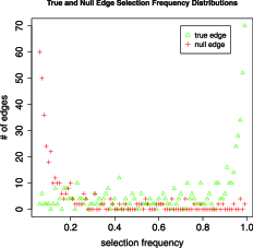
(a)	(b)

Figure 1: The distributions of selection frequencies based on a simulated data set. (a) The distribution of selection frequencies of all edges. (b) Distributions of selection frequencies of null and true edges, respectively (note that these are not observable in practice). Simulation is based on a power-law network with $p=500$, $n=200$, and the number of true edges is 495. The space algorithm with $\lambda=135$ is used as the original nonaggregation procedure $A(\lambda)$. For illustrating the tail behavior of these distributions more effectively, we only show them on the selection frequency range [0.06, 1], as there are too many edges with selection frequency less than 0.06.

For the finite data case, an aggregation-based procedure could also perform better than the original procedure, as illustrated by the following simulation example (the simulation setup is provided in Section 3). Figure 1(a) shows the empirical distribution of selection frequencies based on a simulated data set and Figure 1(b) shows the empirical distributions of true edges (green triangles) and null edges (red crosses). Note that most null edges have low selection frequencies $<0.4$, while most true edges have large selection frequencies $>0.6$. This suggests that with a properly chosen $c$ (say, $c\in[0.4,0.6]$), $S_{c}^{\lambda}$ will select mostly true edges and only a small number of null edges. In fact, by simply choosing the cutoff $c=0.5$, $S_{c}^{\lambda}$ outperforms $A(\lambda)$ in both FDR and power (Figure 2).

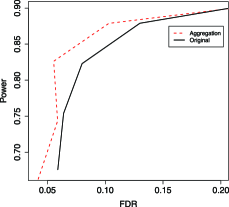
Figure 2: Power and FDR of the aggregation-based procedure $S_{c}^{\lambda}$ with cutoff $c=0.5$ and the original procedure $A(\lambda)$ for $\lambda=96,114,135,160$, with the rest of settings the same as in Figure 1.

2.3 Modeling selection frequency

Now we introduce a mixture model, similar in spirit to Efron (2004a), for estimating the FDR of an aggregation-based procedure $S_{c}^{\lambda}$. We will use this estimate to choose the optimal $c$ and $\lambda$ by controlling FDR while maximizing power. Assume that the selection frequencies $\{X_{ij}^{\lambda},(i,j)\in\Omega\}$, generated from $B$ resamples, fall into two categories, “true” or “null,” depending on whether $(i,j)$ is a true edge or a null edge. Let $\pi$ be the proportion of the true edges. We also assume that $X_{ij}^{\lambda}$ has density $f_{1}^{\lambda}(x)$ or $f_{0}^{\lambda}(x)$ if it belongs to the “true” or the “null” categories, respectively. Note that both $f_{1}^{\lambda}$ and $f_{0}^{\lambda}$ depend on the sample size $n$, but such dependence is not explicitly expressed in order to keep the notation simple. The mixture density for $X_{ij}^{\lambda}$ can be written as

$$f^{\lambda}(x)=(1-\pi)f_{0}^{\lambda}(x)+\pi f_{1}^{\lambda}(x),\qquad x\in\{0,1/B,2/B,\ldots,1\}.$$ (6)

Based on this mixture model, the (positive) FDR [Storey (2003)] of the aggregation-based procedure $S_{c}^{\lambda}$ is

$$\operatorname{FDR}\bigl{(}S_{c}^{\lambda}\bigr{)}=\operatorname{Pr}\bigl{(}(i,j)\in E^{c}|(i,j)\in S_{c}^{\lambda}\bigr{)}=\frac{\sum_{x\geq c}(1-\pi)f_{0}^{\lambda}(x)}{\sum_{x\geq c}f^{\lambda}(x)}.$$ (7)

Given an estimate $\widehat{\operatorname{FDR}}(S_{c}^{\lambda})$ (which will be discussed below) from (7), the number of true edges in $S_{c}^{\lambda}$ can be estimated by

$$\widehat{N}_{E}\bigl{(}S_{c}^{\lambda}\bigr{)}=\bigl{|}S_{c}^{\lambda}\bigr{|}\bigl{(}1-\widehat{\operatorname{FDR}}\bigl{(}S_{c}^{\lambda}\bigr{)}\bigr{)},$$ (8)

which can be used to compare the power of $S_{c}^{\lambda}$ across various choices of $c$ and $\lambda$, as the total number of true edges is a constant. Consequently, for a given targeted FDR level $\alpha$, we first seek for the optimal threshold $c$ for each $\lambda\in\Lambda$,

$$c^{*}(\lambda)=\operatorname{min}\bigl{\{}c\dvtx\widehat{\operatorname{FDR}}\bigl{(}S_{c}^{\lambda}\bigr{)}\leq\alpha\bigr{\}},$$ (9)

and then we find the optimal regularization parameter

$$\lambda^{*}=\mathop{\operatorname{argmax}}_{\lambda\in\Lambda}\widehat{N}_{E}\bigl{(}S_{c^{*}(\lambda)}^{\lambda}\bigr{)},$$ (10)

such that the corresponding procedure $S_{c^{*}(\lambda^{*})}^{\lambda^{*}}$ achieves the largest power among all competitors with estimated FDR not exceeding $\alpha$.

The above procedure depends on a good FDR estimate, which in turn requires good estimates of the mixture density $f^{\lambda}$ and its null-edge contribution $(1-\pi)f_{0}^{\lambda}$. A natural estimator of $f^{\lambda}$ is simply the empirical selection frequencies, that is,

$$\hat{f}^{\lambda}\biggl{(}\frac{k}{B}\biggr{)}=\frac{n^{\lambda}_{k}}{N_{\Omega}},\qquad k=0,1,\ldots,B,$$

where $N_{\Omega}=p(p-1)/2$ is the total number of candidate edges and $n_{k}^{\lambda}=|\{(i,j)\dvtx X_{ij}^{\lambda}=k/B\}|$ is the number of edges with selection frequencies equal to $k/B$.

Before describing an approach to estimating $\pi$ and $f_{0}^{\lambda}$, we note two observations from Figure 1(b). First, the contribution from the true edges to the mixture density $f^{\lambda}$ is small in the range where the selection frequencies are small. Second, the empirical distribution of $f_{0}^{\lambda}$ is monotonically decreasing. These can be formally summarized as the following condition.

There exist $V_{1}$ and $V_{2}$, $0<V_{1}<V_{2}<1$, such that as $n\rightarrow\infty$: [(C1)]

$f_{1}^{\lambda}\rightarrow 0$ on $(V_{1},V_{2}]$;

$f_{0}^{\lambda}$ is monotonically decreasing on $(V_{1},1]$.

This proper condition is satisfied by a class of procedures as described in the lemma below (the proof is provided in the Appendix).

Lemma 1

A selection procedure satisfies the proper condition if, as the sample size increases, $\tilde{p}_{ij}$ tends to one uniformly for all true edges and has a limit superior strictly less than one for all null edges.

Remark 1.

It is easy to verify that all consistent procedures applied to subsampling resamples satisfy the condition in Lemma 1. Other examples are procedures that use randomized lasso penalties [Meinshausen and Bühlmann (2010)]. See Section 2.5 for more details.

The proper condition motivates us to estimate $\pi$ and $f_{0}^{\lambda}$ by fitting a parametric model $g_{\theta}$ for $f^{\lambda}$ in the region $(V_{1},V_{2}]$ and then extrapolating the fit to the region $(V_{2},1]$. This is because if C1 is satisfied, then $(1-\pi)f_{0}^{\lambda}$ can be well approximated based on the empirical mixture density from the region $(V_{1},V_{2}]$. If C2 is also satisfied, the extrapolation of $g_{\theta}$ will be a good approximation to $(1-\pi)f_{0}^{\lambda}$ on $(V_{2},1]$ for a reasonably chosen family of $g_{\theta}$.

We choose the parametric family as follows. Given $\tilde{p}_{ij}$, it is natural to model the selection frequency by a (rescaled) binomial distribution, denoted by $b_{1}(\cdot|\tilde{p}_{ij})$, due to the independent and identical nature of resampling conditional on the original data. Moreover, we use a powered beta distribution [i.e., the distribution of $Q^{\gamma}$ where $Q\sim$ beta$(a,b)$, $a,b,r>0$] as the prior for $\tilde{p}_{ij}$’s, denoted by $b_{2}(\cdot|\theta)$ with $\theta=(a,b,r)$. This is motivated by the fact that the beta family is a commonly used conjugate prior for the binomial family, and the additional power parameter $\gamma$ simply provides more flexibility in fitting. Thus, the distribution of selection frequencies of null edges is modeled as

$$h_{\theta}(x)=\int_{0}^{1}b_{1}(x|\tau)b_{2}(\tau|\theta)\,d\tau.$$

The null-edge contribution $(1-\pi)f_{0}^{\lambda}$ can be estimated by fitting $h_{\theta}$ to the empirical mixture density $\hat{f}^{\lambda}$ in the fitting range $(V_{1},V_{2}]$, which, in practice, is determined based on the shape of $\hat{f}^{\lambda}$ (details are given in Section 2.4). Specifically, we estimate $\pi$ and $f_{0}^{\lambda}$ by $\hat{\pi}$ and $h_{\hat{\theta}}$, via

$$(\hat{\pi},\hat{\theta})=\mathop{\operatorname{argmin}}_{\pi,\theta}L\bigl{(}\hat{f}^{\lambda}(\cdot),(1-\pi)h_{\theta}(\cdot)\bigr{)},$$ (11)

where $L(f,g)\equiv-\sum_{x\in(V_{1},V_{2}]}[f(x)\operatorname{log}g(x)]$, which amounts to the Kullback–Leibler distance.

2.4 Proper regularization range

Following what we propose in Section 2.3, we can evaluate the aggregation-based procedure $S_{c}^{\lambda}$ for different choices of $(\lambda,c)$ with regard to model–selection–based criteria: the FDR and the number of selected true edges. For the range of $\lambda$, we consider those that yield “U-shaped” empirical distributions of selection frequencies, that is, $\hat{f}^{\lambda}$ decreases in the small-selection-frequency range and then increases in the large-selection-frequency range [see Figure 1(a) and Figure 3 for examples of “U-shaped” distribution]. The decreasing trend is needed for the proper condition to hold, while the increasing trend helps to control the FDR, since an $S_{c}^{\lambda}$ with $\operatorname{FDR}\leq\alpha$ implies, by (7), that

$$\sum_{x\geq c}f^{\lambda}(x)\geq\frac{(1-\pi)\sum_{x\geq c}f_{0}^{\lambda}(x)}{\alpha}.$$ (12)

U-shape detection procedure
1.	INPUT $\hat{f}^{\lambda}$, the empirical density of selection frequencies. Set $U=1$ (the U-shape indicator).
2.	Check U-shape.
	2.1. Check valley point.
	2.1.1. Calculate $v_{2}=\operatorname{argmin}_{x}\tilde{f}^{\lambda}(x)$, the valley point position,
	where $\tilde{f}^{\lambda}$ is a smooth curve fitted based on $\hat{f}^{\lambda}$. (We use
	the R-function $\tt{smooth.spline()}$, where the degree of
	freedom parameter is determined such that the derivative
	of $\tilde{f}^{\lambda}$ has only one sign change.)
	2.1.2. IF $v_{2}>0.8$
	Set $U=0$, GOTO Step 3.
	END IF
	2.2. Calculate $v_{1}=\operatorname{argmax}_{x<v_{2}}\hat{f}^{\lambda}(x)$, the peak before $v_{2}$.
	2.3. Check if $\hat{f}^{\lambda}$ is “roughly” decreasing on $(v_{1},v_{2}]$.
	2.3.1. Calculate $\mu_{1}=(v_{1}+v_{2})/2$, $s_{1}=\sum_{x\in[v_{1},\mu_{1}]}\hat{f}^{\lambda}(x)$ and
	$s_{2}=\sum_{x\in[\mu_{1},v_{2}]}\hat{f}^{\lambda}(x)$.
	2.3.2. IF $s_{1}<s_{2}$
	Set $U=0$, GOTO Step 3.
	END IF
	2.4. Check if $\hat{f}^{\lambda}$ is “roughly” increasing on $(v_{2},1]$.
	2.4.1. Calculate $\mu_{2}=(v_{2}+1)/2$, $s_{3}=\sum_{x\in[v_{2},\mu_{2}]}\hat{f}^{\lambda}(x)$ and
	$s_{4}=\sum_{x\in[\mu_{2},1]}\hat{f}^{\lambda}(x)$.
	2.4.2. IF $s_{3}>s_{4}$
	Set $U=0$, GOTO Step 3.
	END IF
3.	RETURN $v_{1},v_{2},U$.

Therefore, if $\hat{f}^{\lambda}$ is not sufficiently large at the tail, $\operatorname{FDR}\leq\alpha$ may not be achieved for a small value of $\alpha$. The increasing trend also helps to obtain decent power since it guarantees a substantial size of $S_{c}^{\lambda}$. Based on our experience, the $\lambda$ values chosen based on (9) and (10) indeed always corresponds to a “U-shaped” empirical selection frequency distribution.

Thus, we propose the following simple procedure for identifying “U-shaped” $\hat{f}^{\lambda}$’s to determine the proper regularization range in practice. An illustration for this procedure is given in Figure 3.

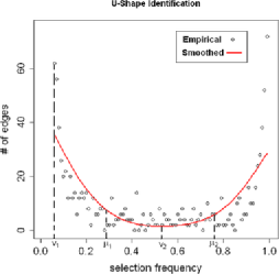
Figure 3: An illustration for the proposed U-shape identification procedure. The empirical distribution ($\hat{f}^{\lambda}$) is the same as the one in Figure 1. The smooth curve ($\tilde{f}^{\lambda}$) is fitted by the R-function $\tt{smooth.spline}$ with df${}=4$. Locations of $v_{1}$, $v_{2}$, $\mu_{1}$ and $\mu_{2}$ are found by following steps in the U-shape detection procedure.

Remark 2.

Step 2.1 is based on our extensive simulation where we find that a large value of $v_{2}$ often corresponds to a too-small $\lambda$, yielding too many null edges with high selection frequencies, which makes (12) difficult to hold for reasonably small FDR levels $\alpha$ (see Section D1 in the supplemental article [Li et al. (2013)]). If $\hat{f}^{\lambda}$ is not recognized as “U-shaped” for a large range of $\lambda$’s, we would consider the data as lack of signals where a powerful $S_{c}^{\lambda}$ is not attainable. One example is the empty network (see Section 3.2 and Figure S-1 in the supplemental article [Li et al. (2013)]).

Sections 2.2–2.4 provide a procedure for network inference based on directly estimating FDR. We name the procedure as BINCO—Bootstrap Inference for Network COnstruction, as we suggest to use bootstrap resamples. The main steps are summarized below.

2.5 Randomized lasso

For an $L_{1}$ regularized procedure $A(\lambda)$, the proper condition (Section 2.3) is satisfied if $A(\lambda)$ is selection consistent, which usually requires strong conditions, for instance, the well-known irrepresentable condition under the lasso regression setting [Zhao and Yu (2006), Zou (2006), Yuan and Lin (2007), Wainwright (2009)] or the so-called neighborhood stability condition under the GGM setting [Meinshausen and Bühlmann (2006), Peng et al. (2009)]. Recently, Meinshausen and Bühlmann (2010) proposed the randomized lasso, which is a procedure based on randomly sampled regularization parameters. For example, the randomized lasso version of space would be

$$\qquad L(Y,\theta,W)=\frac{1}{2}\Biggl{\{}\sum_{i=1}^{p}\biggl{\|}Y_{i}-\sum_{j:j\not=i}\sqrt{\frac{\sigma_{jj}}{\sigma_{ii}}}\rho_{ij}Y_{j}\biggr{\|}^{2}\Biggr{\}}+\lambda\sum_{1\leq i<j\leq p}|\rho_{ij}|/w_{ij},$$ (13)

BINCO procedure
1.	INPUT $\Lambda=(\lambda_{1},\ldots,\lambda_{k})$ the initial range of regularization parameter values; $Y_{n\times p}$ the dataset; and $\alpha$ the desired FDR level.
2.	FOR $i=1$ TO $k$
	2.1. $\lambda=\lambda_{i}$
	2.2. Generate $\hat{f}^{\lambda}$ the empirical density of selection frequencies.
	2.3. Check whether $\hat{f}^{\lambda}$ is U-shaped based on the output $(v_{1},v_{2},U)$ from
	the “U-Shape Detection Procedure.”
	2.4. IF $\hat{f}^{\lambda}$ is U-shaped (i.e., $U=1$)
	2.4.1. Obtain the null density estimate $\hat{f}^{\lambda}_{0}$ by (11).
	2.4.2. Find the optimal threshold $c^{*}(\lambda)$ by (9), where the FDR
	is estimated based on (7) with $f^{\lambda}$ and $f^{\lambda}_{0}$ replaced by $\hat{f}^{\lambda}$
	and $\hat{f}^{\lambda}_{0}$,respectively.
	2.4.3. Obtain $S_{c^{*}(\lambda)}^{\lambda}$ and calculate $\hat{N_{E}}(S_{c^{*}(\lambda)}^{\lambda})$, the estimated
	number of true edges being selected, based on (8).
	END IF
	ELSE $\hat{N_{E}}(S_{c^{*}(\lambda)}^{\lambda})=0$, $S_{c^{*}(\lambda)}^{\lambda}=\emptyset$.
	2.5. OUTPUT $\hat{N_{E}}(S_{c^{*}(\lambda)}^{\lambda})$ and $S_{c^{*}(\lambda)}^{\lambda}$.
	NEXT $i$
3.	Determine the optimal regularization $\lambda^{*}$ through (10). The optimal selection is $S_{c^{*}(\lambda^{*})}^{\lambda^{*}}$.

where $w_{ij}$’s are randomly sampled from a probability distribution $p(w)$ supported on $(l,1]$ for some $l\in(0,1]$ (note that $l=1$ corresponds to the ordinary$L_{1}$ penalty). The advantage of this randomized lasso procedure is that, by perturbing the regularization parameters, the irrelevant features may be decorrelated from the true features in some configurations of randomly sampled weights such that the irrepresentable condition is satisfied. Therefore, it selects all true features with probability tending to 1 and any irrelevant feature with a limiting probability strictly less than 1. As a result, a consistent aggregation-based procedure can be achieved under conditions “typically much weaker than the standard assumption of the irrepresentable condition” [Meinshausen and Bühlmann (2010), Theorem 2]. For this case, based on Lemma 1, the proper condition is also satisfied.

If (13) is used as the original (nonaggregated) procedure, an additional parameter $l$, which controls the amount of perturbation of the regularization parameter, needs to be chosen. A small $l$ guards better against false positives but damages power, while a large $l$ may result in a liberal procedure. Here we provide a two-step data-driven procedure for choosing an appropriate $l$ in BINCO. We first fix $l=1$, that is, the ordinary $L_{1}$ penalty, to find a proper range $\Lambda^{*}$ for $\lambda$ that corresponds to the “U-shaped” empirical mixtures. Then for each $\lambda\in\Lambda^{*}$, we consider a set of pairs $\Lambda_{2}=\{(\lambda_{i},l_{i}),i=1,\ldots,m\}$ such that $\int_{l_{i}}^{1}\frac{\lambda_{i}}{w}p(w)\,dw=\lambda$, that is, keeping the average amount of regularization unchanged. For example, in the simulation study, we use $l_{i}=i/10,i=1,\ldots,9$. We then pick the pair $(\lambda^{*},l^{*})\in\Lambda_{2}$ such that $l^{*}$ is the smallest among those $l$’s that yield U-shaped empirical mixture distributions. Our simulation shows that such a choice of $(\lambda^{*},l^{*})$ ensures good power for BINCO while controlling FDR in a slightly conservative fashion.

3 Simulation

In this section we first compare the performance of BINCO with stability selection [Meinshausen and Bühlmann (2010)], and then investigate the performance of BINCO with respect to various factors, including the network structure, dimensionality, signal strength and sample size.

We use space [Peng et al. (2009)] coupled with randomized lasso (13) as the original nonaggregate procedure, where the random weights $\frac{1}{w_{ij}}$’s are generated from the uniform distribution $U[1,1/l]$ for $l\in(0,1]$. The selection frequencies are obtained based on $B=100$ resamples. Since subsampling of size $[n/2]$ is proposed for stability selection, we use subsampling to generate resamples when comparing BINCO and stability selection. For investigating BINCO’s performance, we use bootstrap resamples because it yields slightly better performance (see Remark 4).

The performance of both methods are evaluated by true FDRs and power, since for simulations we know whether an edge is true or null. In addition, we define ideal power, which is the best power one can achieve for $S_{c}^{\lambda}$ given the true $\operatorname{FDR}\leq\alpha$ (in simulation we consider $\alpha=0.05$ and $\alpha=0.1$). Based on ideal power, we can evaluate the efficiency of the methods under different settings. For each simulation setting, results are based on 20 independent simulation runs.

3.1 Comparison between BINCO and stability selection

Stability selection procedure selects $S_{\mathrm{stable}}^{\Lambda}(t)\equiv\{(i,j)\dvtx\operatorname{max}_{\lambda\in\Lambda}(X_{ij}^{\lambda})\geq t\}$, a set of edges with the maximum selection frequency over a prespecified regularization set $\Lambda$ exceeding a threshold $t$. Assuming an exchangeability condition upon the irrelevant variables (here the null edges), Meinshausen and Bühlmann [(2010), Theorem 1] derived an upper bound for the expected number of falsely selected variables for each choice of $t>0.5$. Specifically, under suitable conditions, the expected number of null edges selected by the set $S_{\mathrm{stable}}^{\Lambda}(t)$, denoted by $E(V)$, satisfies

$$E(V)\leq\frac{q_{\Lambda}^{2}}{(2t-1)N_{\Omega}},$$ (14)

where $N_{\Omega}=p(p-1)/2$ is the total number of candidate edges and $q_{\Lambda}$ is the expected number of edges selected under at least one $\lambda\in\Lambda$. In practice, $q_{\Lambda}$ can be estimated by $\frac{1}{B}\sum_{i=1}^{B}|\bigcup_{\lambda\in\Lambda}S^{\lambda}(Y^{i})|$. Dividing both sides of (14) by $|S_{\mathrm{stable}}^{\Lambda}(t)|$, we obtain

$$\frac{E(V)}{|S_{\mathrm{stable}}^{\Lambda}(t)|}\leq\frac{q_{\Lambda}^{2}}{(2t-1)N_{\Omega}\cdot|S_{\mathrm{stable}}^{\Lambda}(t)|}.$$ (15)

Although stability selection is intended to control $E(V)$, for an easier comparison with BINCO, we use $\frac{E(V)}{|S_{\mathrm{stable}}^{\Lambda}(t)|}$ to approximate FDR and obtain the optimal $S_{\mathrm{stable}}^{\Lambda}(t)$ by finding the smallest threshold $t$ such that the upper bound on the right-hand side of (15) is less than or equal to $\alpha$.

For data generation, we first consider a power-law network with $p=500$ nodes whose degree (i.e., the number of connected edges for each node) distribution follows $P(k)\sim k^{-\gamma}$. The scaling exponent $\gamma$ is set to be 2.3, which is consistent with the findings in the literature for biological networks [Newman (2003)]. There are in total 495 true edges in this network and its topology is illustrated in Figure 5(a). The sample size is $n=200$. Two settings with different signal strengths are considered: (1) strong signal, the mean and standard deviation (SD) of nonzero $|\rho_{ij}|$’s are 0.34 and 0.13, respectively; (2) weak signal, the mean and SD of nonzero $|\rho_{ij}|$’s are 0.25 and 0.09, respectively. Note both positive and negative correlations are allowed in this network.

We compare the performance of BINCO and stability selection at a targeted FDR level of 0.05. For BINCO, we consider $\Lambda_{0}=\{40,50,\ldots,100\}$ as the initial range for $\lambda$ and then obtain the optimal final selection following the steps at the end of Section 2.4. For stability selection, since no specific guidance was provided for choosing $\Lambda$ and $l$ (the randomized lasso regularization perturbation parameter), we consider three different values for $l\in\{0.5,0.8,1\}$ and a collection of intervals $\Lambda=(\lambda_{\operatorname{min}},\lambda_{\operatorname{max}})$ with $\lambda_{\operatorname{min}}$ varying from 40 to 100 and $\lambda_{\operatorname{max}}=100$. This choice of $\Lambda$ is due to the fact that the upper bound in (15) cannot be controlled at 0.05 for any $t$ for $\lambda_{\operatorname{min}}<40$, and the performance of stability selection is largely invariant for $\lambda_{\operatorname{max}}$.

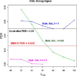
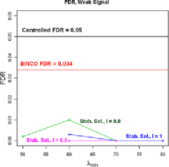
(a)	(b)
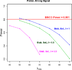
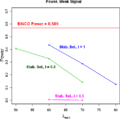
(c)	(d)

Figure 4: The FDR (top panels) and power (bottom panels) for BINCO and stability selection (Stab. Sel.). (a) and (c) are for the strong signal setting; (b) and (d) are for the weak signal setting.

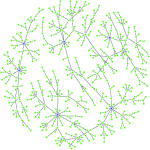
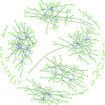
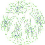
(a)	(b)	(c)

Figure 5: Different network topologies: (a) Power-law network, number of true edges${}=495$; (b) Empirical network, number of true edges${}=633$; (c) Hub network, number of true edges${}=587$. All three networks have $p=500$ nodes.

When the signals are strong, BINCO gives a conservative $\operatorname{FDR}=0.026$ but still maintains good power${}=0.801$ [Figures 4(a) and 4(c)]. The performance of stability selection varies for different choices of $\lambda_{\operatorname{min}}$ and $l$. The FDRs are larger than the targeted level 0.05 for some $\lambda_{\operatorname{min}}$’s when $l=0.8$ and for all $\lambda_{\operatorname{min}}$’s when $l=1$. For other cases (some $\lambda_{\operatorname{min}}$’s when $l=0.8$ and all $\lambda_{\operatorname{min}}$’s when $l=0.5$), the FDR control is very conservative and the corresponding power is consistently lower than BINCO. When the signals are weak, stability selection is much more conservative than BINCO and results in much lower power [Figures 4(b) and 4(d)]. In Table 1 we report the ideal power, the power for BINCO and the best power for stability selection (among different choices of $\lambda_{\operatorname{min}}$) under $l=0.5$, 0.8 and 1. We also calculate the power efficiency as the ratio of the power for the method over the ideal power, for BINCO and stability selection, respectively. It can be seen that the power of BINCO is close to the ideal power for both levels of signal strength, while stability selection is too conservative when the signal strength is weak. For more detailed results, see Section A1 in the supplemental article [Li et al. (2013)].

Remark 3.

In some cases we find that stability selection fails to control FDR. We suspect this may be due to the violation of the exchangeability assumption in Theorem 1 of Meinshausen and Bühlmann (2010). We examine the impact of the exchangeability assumption by simulation and find that when it is violated, the theoretical upper bound in (14) for $E(V)$ may not hold (see Section D2 in the supplemental article [Li et al. (2013)] for further details).

3.2 Further investigation of BINCO

Now we investigate the effects of the network structure, dimensionality, signal strength and sample size on the performance of BINCO.

Table 1: Power comparison between BINCO and stability selection under strong and weak signals

				Stability selection
		Idealtt1	BINCO	$\bolds{l=1}$	$\bolds{l=0.8}$	$\bolds{l=0.5}$
Strong signal	Power	0.853	0.801	0.818tt3	0.785tt3	0.706
	MPEtt2	100.0	0.939	0.959tt3	0.920tt3	0.828
Weak signal	Power	0.616	0.569	0.4340	0.4070	0.170
	MPEtt2	100.0	0.924	0.7050	0.6610	0.276

[1]tt1“Ideal” refers to the ideal power that can be achieved when the true distribution of null edges is known. [2]tt2Method Power Efficiency (MPE)${}={}$method power${}/{}$ideal power. [3]tt3FDR control failed.

Network structure.

We consider four different network topologies: empty network, power-law network, empirical network and hub network. In each network there are five disconnected components with 100 nodes each. Below is a brief description of the network topologies:

[(1)]

Empty network: there is no edge connecting any pair of nodes.

Power-law network: the degree follows a power-law distribution with parameter $\gamma=2.3$ as described in Section 3.1 [Figure 5(a)].

Empirical network: the topology is simulated according to an empirical degree distribution of one genetic regulatory network [Schadt et al. (2005)] [Figure 5(b)].

Hub network: three nodes per component have a large number of connecting edges ($>$15) and all other nodes have a small number of connecting edges ($<$5) [Figure 5(c)].

We set the sample size $n=200$. The signal strength for all networks except for the empty network is fixed at the strong level as in Section 3.1.

Table 2: Investigation of the impact of different networks on BINCO performance

	Targeted $\bolds{\operatorname{FDR}=0.05}$				Targeted $\bolds{\operatorname{FDR}=0.10}$
	FDR		Power		FDR		Power
Network topology	Mean	SD	Mean	SD	Mean	SD	Mean	SD
Power-law	0.046	0.009	0.810	0.013	0.096	0.013	0.845	0.013
Empirical	0.032	0.019	0.523	0.040	0.068	0.034	0.565	0.040
Hub	0.023	0.009	0.644	0.021	0.052	0.012	0.692	0.017

Table 3: Comparison of BINCO power and ideal power under different networks

	Targeted $\bolds{\operatorname{FDR}=0.05}$			Targeted $\bolds{\operatorname{FDR}=0.10}$
Topology	Power-law	Empirical	Hub	Power-law	Empirical	Hub
BINCO power	0.810	0.523	0.644	0.845	0.565	0.692
Ideal power	0.856	0.595	0.736	0.881	0.631	0.776
MPEttt1	0.946	0.879	0.875	0.959	0.895	0.892

[1]ttt1Method Power Efficiency (MPE)${}={}$method power${}/{}$ideal power.

For the empty network, the empirical mixture distributions of selection frequencies monotonically decrease on a wide range of $\lambda$ (Figure S-1) and are not recognized by BINCO as “U-shaped.” Thus, we reach the correct conclusion that there is no signal in this case. In contrast, data sets from the other three networks produce the desired “U-shaped” mixture distributions for some $\lambda$ (Figure S-2).

We compare BINCO results across networks 2-4 with FDR targeted at level $\alpha=0.05$ and 0.1. BINCO gives slightly conservative control on FDR and achieves reasonable power for all three networks (Table 2). The comparison to the ideal power shows that the network topologies investigated here have only a small effect on BINCO’s efficiency (Table 3).

Dimensionality. We investigate the impact of dimensionality on the performance of BINCO. We consider the power-law network and let the number of nodes $p$ vary from 500, 800 to 1000. To keep the complexity of each component the same across different choices of $p$, we set the component size constant, being 100, and the number of components $C=p/100$. Again the sample size $n=200$ is used for all three cases and the signal strength is fixed at the strong level as in Section 3.1.

For all three choices of $p$, BINCO performs similarly (Table 4), with slightly conservative FDR and power around 0.8. The dimensionality does not demonstrate a significant impact on BINCO. BINCO’s result is also largely invariant when we compare networks of differing numbers of components with $p$ fixed (such that component size varies, see Section A3 in the supplemental article [Li et al. (2013)]).

Table 4: Investigation of the impact of different dimensionality on BINCO performance

	Targeted $\bolds{\operatorname{FDR}=0.05}$				Targeted $\bolds{\operatorname{FDR}=0.10}$
	FDR		Power		FDR		Power
Dimension $\bolds{p}$	Mean	SD	Mean	SD	Mean	SD	Mean	SD
500	0.046	0.009	0.810	0.013	0.096	0.013	0.845	0.013
800	0.030	0.007	0.769	0.010	0.083	0.010	0.811	0.012
1000	0.043	0.007	0.784	0.008	0.096	0.011	0.821	0.007

Table 5: Investigation of the impact of different signal strength on BINCO performance

	Targeted $\bolds{\operatorname{FDR}=0.05}$				Targeted $\bolds{\operatorname{FDR}=0.10}$
	FDR		Power		FDR		Power
Signal strength	Mean	SD	Mean	SD	Mean	SD	Mean	SD
Strong	0.046	0.009	0.810	0.013	0.096	0.013	0.845	0.013
Weak	0.032	0.010	0.579	0.024	0.063	0.014	0.617	0.018
Very weak	0.035	0.026	0.252	0.040	0.065	0.037	0.310	0.039

Signal strength. We consider three levels of signal strength: strong, weak and very weak. The corresponding means and SDs of nonzero $|\rho_{ij}|$’s are $(0.34,0.13)$, $(0.25,0.09)$ and $(0.21,0.07)$, respectively. The network is the power-law network with $p=500$ and sample size is $n=200$ for all settings.

BINCO provides good control on FDR, however, the power decreases from 0.8 to 0.3 as the signal weakens (Table 5). Comparing the power of BINCO with the ideal power (Table 6), we see that BINCO remains efficient and the loss in power is largely due to reduction of signal strength.

Table 6: Power comparison of BINCO power and ideal power when the signal strength is strong, weak and very weak

	Targeted $\bolds{\operatorname{FDR}=0.05}$			Targeted $\bolds{\operatorname{FDR}=0.10}$
Signal strength	Strong	Weak	Very weak	Strong	Weak	Very weak
BINCO power	0.810	0.579	0.252	0.845	0.617	0.310
Ideal power	0.856	0.615	0.279	0.881	0.651	0.345
MPEtttt1	0.946	0.941	0.903	0.959	0.948	0.899

[1]tttt1Method Power Efficiency (MPE)${}={}$method power${}/{}$ideal power.

Sample size. Now we consider the impact of sample size $n$ by varying it from 200, 500 and 1000, while keeping the signal strength at the “very weak” level as in the previous simulation. The network structure is again the power-law network with $p=500$.

With an increased sample size, the power of BINCO is significantly improved from 0.3 to nearly 0.9 while the FDRs are well controlled (Table 7).

Table 7: Investigation of the impact of different sample size on BINCO performance

	Targeted $\bolds{\operatorname{FDR}=0.05}$				Targeted $\bolds{\operatorname{FDR}=0.10}$
	FDR		Power		FDR		Power
Sample size	Mean	SD	Mean	SD	Mean	SD	Mean	SD
200	0.035	0.026	0.252	0.040	0.065	0.037	0.310	0.039
500	0.024	0.010	0.684	0.012	0.049	0.011	0.714	0.014
1000	0.045	0.010	0.869	0.013	0.090	0.015	0.891	0.012

In summary, BINCO has good control for FDR under a wide range of scenarios. Its performance is shown to be robust for networks with different topologies and dimensionalities, and its efficiency is not influenced much even when the signal strength is weak. As the sample size increases, the power of BINCO is improved significantly.

Remark 4.

We propose to use bootstrap over subsampling, as the former appears to give slightly better power. Intuitively, bootstrap contains more distinct samples [0.632$n$, Pathak (1962)] than $[n/2]$ subsampling (0.5$n$). However, the difference we have observed is rather small. For example, we compare the power over 20 independent samples between bootstrap and $[n/2]$ subsampling under the power-law network setting. For $\operatorname{FDR}=0.05$, the power is 0.810 for bootstrap and 0.801 for subsampling (compare Tables 3 and 1); while for $\operatorname{FDR}=0.1$, the power is 0.845 for bootstrap and 0.835 for subsampling [compare Tables 3 and S-7 from Li et al. (2013)]. This observation is in agreement with the conclusions of several others [Menshausen and Bühlmann (2010), Freedman (1977), Bühlmann and Yu (2002)].

4 A real data application

We apply the BINCO method to a microarray expression data set of breast cancer (BC) [Loi et al. (2007)] to build a gene expression network related to the disease. The data (http://www.ncbi.nlm. nih.gov/geo/query/acc.cgi?acc=GSE6532) contains measurements of expression levels of 44,928 probes in tumor tissue samples from 414 BC patients based on the Affymetrix Human Genome U133A, U133B and U133 plus 2.0 Microarray platforms.

We preprocess the data as follows. First, a global normalization is applied by centering the median of each array to zero and scaling the Median Absolute Deviation (MAD) to one. Probes with standard deviation (SD) greater than the $25\%$-trimmed mean of all SDs are selected. We further focus on a subset of $1257$ probes for genes from cell cycle and DNA-repair related pathways (http://peiwang.fhcrc.org/internal/papers/DNArepair_CellCircle_related.csv/view), as these pathways have been shown to play significant roles in BC tumor initiation and development. Clinical information including age, tumor size, ER-status (positive or negative) and treatment status (tamoxifen treated or not) is incorporated in the analysis as “fake genes” since we are also interested in investigating whether gene expressions are associated with these clinical characteristics. Finally, we standardize each expression level to have mean zero and SD one. The resulting data set has $p=1261$ genes/probes (including four clinical variables) and $n=414$ tumor samples.

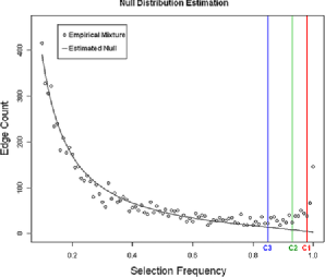
Figure 6: The empirical selection frequency distribution of all edges (dots) and the estimated selection frequency distribution of null edges (solid line). The three vertical lines are drawn at the cutoffs $C1=0.98$, $C2=0.93$ and $C3=0.85$ for FDR at 0.05, 0.1 and 0.2, respectively.

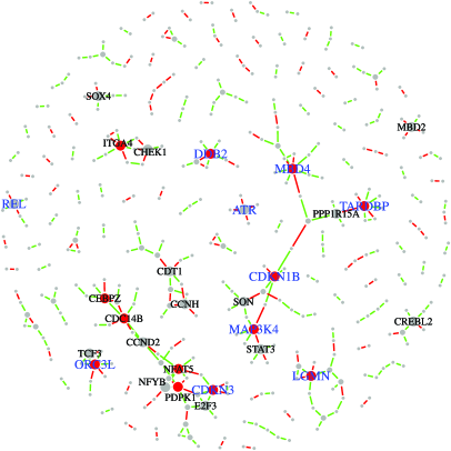
Figure 7: Inferred networks at $\operatorname{FDR}=0.2$ from the BC expression data. A total of 338 edges (selection frequencies $\geq 0.85$) are identified. Among these 338 edges, those with selection frequencies $\geq 0.98$ (corresponding to the set with $\operatorname{FDR}=0.05$) are colored in red, while other edges are colored in green. Genes with degree${}>$3 are labeled by their symbols; genes with degree${}>$4 are indicated by red nodes. In addition, the top ten genes with consistently high connection across perturbed data sets are labeled in blue symbols.

We generate selection frequencies by applying the space algorithm with randomized lasso regularization to $B=100$ bootstrap resamples. The initial range of the tuning parameter $\lambda$ is set to be $\Lambda=(100,120,\ldots,580)$. We then apply the BINCO procedure and find that the optimal values for the regularization parameters are $\lambda=340$ and $l=0.9$. The empirical distribution of selection frequencies of all edges and the null density estimation are given in Figure 6. When the estimated FDR is controlled at 0.05, 0.1 and 0.2, BINCO identifies 125, 222 and 338 edges, respectively. The estimated network for $\operatorname{FDR}=0.2$ is shown in Figure 7. In this figure, two components of a large connectivity structure are observed. They contain most of the genes that are connected by a large number of high-selection-frequency edges. This constructed network can help to generate a useful biological hypothesis and to design follow-up experiments to better understand the underlying mechanism in BC. For example, BINCO suggests with high confidence for the association between MAP3K4 and STAT3. MAP3K4 plays a role in the signal transduction pathways of BC cell proliferation, survival and apoptosis [Bild and Johnson (2001)], and the constitutive activation of STAT3 is also frequently detected in BC tissues and cell lines [Hsieh, Cheng and Lin (2005)]. Interestingly, both MAP3K4 and STAT3 play roles in the regulation of c-Jun, a novel candidate oncogene whose aberrant expression contributes to the progression of breast and other human cancers [Tront, Hoffman and Liebermann (2006); Shackleford et al. (2011)]. The association between MAP3K4 and STAT3 detected by BINCO suggests their potential cooperative roles in BC. It is also worth noting that for the four clinical variables, the only edge with high selection frequency is the one between age and ER-status (selection frequency $=0.96$). All edges between clinical variables and the genes/probes are insignificant (selection frequencies $<0.12$).

Networks built on perturbed data sets can also be used to detect hub genes (i.e., highly connected genes), which are often of great interest due to the central role these genes may play in genetic regulatory networks. The idea is to look for genes that show consistent high connection in estimated networks across perturbed data sets. Here, we propose to detect hub genes by the ranks of their degrees based on the estimated networks using $\lambda=340$ and $l=0.9$. The ten genes with the largest means and the smallest SDs of the degree rank across 100 bootstrap resamples (see Figure S-3, in black dots) are MBD4, TARDBP, DDB2, MAP3K4, ORC3L, CDKN1B, REL, ATR, LGMN and CDKN3. Nine out of these ten genes have been reported relevant to BC, while the remaining one (TARDBP) is newly discovered to be related to cancer [Postel-Vinay et al. (2012)], although its role in BC is not clear at present. The neighborhood topologies of these hub genes in the network estimated by BINCO are illustrated in Figure 7. More details of these hub genes are given in the supplemental article [Li et al. (2013)], Section B.

5 Discussion

In this paper we propose the BINCO procedure to conduct high-dimensional network inference. BINCO employs model aggregation strategies and selects edges by directly controlling the FDR. This is achieved by modeling the selection frequencies of edges with a two-component mixture model, where a flexible parametric distribution is used to model the density for the null edges. By doing this, BINCO is able to provide a good estimate of FDR and hence properly controls the FDR. To ensure BINCO works, we propose a set of screening rules to identify the U-shape characteristic of empirical selection frequency distributions. Based on our experience, a U-shape corresponds to a proper amount of regularization such that the FDR is well controlled and the power is reasonable. Extensive simulation results show that BINCO performs well under a wide range of scenarios, indicating that it can be used as a practical tool for network inference. Although we focus on the GGM construction problem in this paper, BINCO is applicable to a wide range of problems where model selection is needed because it provides a general approach to modeling the selection frequencies.

We use a mixture distribution with two components, one corresponding to true edges and the other corresponding to null edges, to model the selection frequency distribution. This two-component mixture model is adequate as long as the distribution of the null component is identifiable and can be reasonably estimated, as formalized in the proper condition. Note that the proper condition holds for a wide range of commonly used (nonaggregation) selection procedures (Lemma 1, Remark 1). To further ensure the FDR can be controlled at a reasonable level, we propose a U-shape detection procedure and only apply BINCO if the empirical distribution of selection frequencies passes the detection. These rules for U-shape detection are empirical but appear to work very well based on our extensive simulations.

BINCO works well despite the presence of correlations between edges (see Section D1 in the supplemental article [Li et al. (2013)]), because we use the independence of edges only as a working assumption . It is well known that if the marginal distribution is correctly specified, the parameter estimates are consistent even in the presence of correlation. This is similar to the generalized estimating equations, where if the mean function is correctly specified, the parameters will be consistently estimated [Liang and Zeger (1986)]. Toward this end, we use the three-parameter power beta distribution to allow for adequate flexibility in modeling the marginal distribution of selection frequencies.

BINCO is computationally feasible for high-dimensional data. The major computational cost lies in generating the selection frequencies via resampling. For each resample, the computational cost is determined by that of the nonaggregated procedure BINCO coupled with. In terms of space, it is $O(np^{2})$. The processing time for a data set with $n=200$, $p=500$, under a given $\lambda$ and 100 bootstrap samples to generate selection frequencies is about 20 minutes on a PC with Pentium dual-core CPU at 2.8 GHz and 1 G ram. These selection frequencies can be simultaneously generated through parallel computing for different $\lambda$’s and weights. Fitting the mixture model takes much less time, which is about 2 minutes for the above example on the same computer.

Although we use GGM as our motivating example, BINCO works well even if the multivariate normality assumption does not hold. Note that the multivariate normality assumption only concerns the interpretation of the edges. Under GGM, the presence of an edge means conditional dependency of the corresponding nodes given all other nodes. Without the normality assumption, one can only conclude nonzero partial correlation between the two nodes given the rest of the nodes. The space method used in this paper is to estimate the concentration network (where an edge is drawn between two nodes if the corresponding partial correlation is nonzero) and has been shown to work well under nonnormal cases such as multivariate-$t$ distributions [Peng et al. (2009)]. We also generate data from nonnormal distributions and found that BINCO works well in this situation (see Section D4 in the supplemental article [Li et al. (2013)]).

BINCO is an aggregation-based procedure. In principle, it can be coupled with any selection procedure. In this sense, it has a wide range of applications as long as the features are defined (e.g., edges as in this paper, variables or canonical correlations as in the example below) and the selection procedure is reasonably good, for example, producing probabilities that satisfy the condition in Lemma 1. One application beyond GGM could be on the multi-attribute network construction where the links/edges are defined based on canonical correlations [Waaijenborg, Verselewel de Witt Hamer and Zwinderman (2008), Katenka and Kolaczyk (2012), Witten, Tibshirani and Hastie (2009)]. Another interesting extension may be on the time-varying network construction [Kolar et al. (2010)] where appropriate incorporation of the time-domain structure across aggregated models will be important. These are beyond the scope of this paper and will be pursued in future research.

The R package BINCO is available through CRAN.

Appendix: Proof of Lemma 1

Suppose as the sample size $n$ increases, an edge selection procedure $A(\lambda)$ gives selection probabilities $\{\tilde{p}^{(n)}_{ij}\}$ (with respect to resample space) which uniformly satisfy

$$\tilde{p}^{(n)}_{ij}\rightarrow 1\qquad\mbox{if }(i,j)\in E$$ (.1)

and

$$\limsup\tilde{p}^{(n)}_{ij}\leq M<1\qquad\mbox{if }(i,j)\in E^{c}.$$ (.2)

Suppose $B$ is large such that $\frac{B+1}{B}M<1$. Let $X$ be a random sample from the set of selection frequencies $\{X_{ij}^{\lambda}\}$ generated by applying $A(\lambda)$ on $B$ resamples, that is, $\operatorname{Pr}(X=X_{ij}^{\lambda})=1/N_{\Omega}$, $(i,j)\in\Omega$. Also suppose $X$ has density $f_{ij}^{\lambda}$ if $X=X_{ij}^{\lambda}$. Then the mixture model (6) becomes

$$f^{\lambda}(x) = (1-\pi)f_{0}^{\lambda}(x)+\pi f_{1}^{\lambda}(x)$$

$$= \sum_{(i,j)\in E^{c}}\frac{1}{N_{\Omega}}f_{ij}^{\lambda}(x)+\sum_{(i,j)\in E}\frac{1}{N_{\Omega}}f_{ij}^{\lambda}(x)$$

with $(1-\pi)f_{0}^{\lambda}(x)=\sum_{(i,j)\in E^{c}}\frac{1}{N_{\Omega}}f_{ij}^{\lambda}(x)$ and $\pi f_{1}^{\lambda}(x)=\sum_{(i,j)\in E}\frac{1}{N_{\Omega}}f_{ij}^{\lambda}(x)$.

Because of the i.i.d. nature of resamples given the data, $f_{ij}^{\lambda}$ is a binomial density with $\tilde{p}_{ij}^{(n)}$ as the probability of success, that is, $f_{ij}^{\lambda}(x)={B\choose k}(\tilde{p}_{ij}^{(n)})^{k}(1-\tilde{p}_{ij}^{(n)})^{B-k}$ for $x=k/B,k=0,1,\ldots,B$. This binomial density is monotone decreasing for $x$ greater than its mode $\mu_{ij}=\frac{[(B+1)\tilde{p}_{ij}^{(n)}]}{B}$ or $\frac{[(B+1)\tilde{p}_{ij}^{(n)}]-1}{B}$. By (.2), given $V_{1}=\frac{B+1}{B}M<1$ and $\varepsilon>0$ such that $V_{1}+\varepsilon<1$, $\exists N$ such that for all $n>N$ $\operatorname{max}_{(i,j)\in E^{c}}(\mu_{ij})<V_{1}+\varepsilon$ and hence for any null edge $(i,j)\in E^{c}$, $f_{ij}^{\lambda}(x)$ is monotone decreasing on $[V_{1}+\varepsilon,1]$, which implies C2 since $f_{0}^{\lambda}(x)=\frac{1}{(1-\pi)N_{\Omega}}\sum_{(i,j)\in E^{c}}f_{ij}^{\lambda}(x)$. Also, (.1) implies, for $(i,j)\in E$, $f_{ij}^{\lambda}(x)\rightarrow 0$ uniformly for $x<1$, which implies C1 for any $V_{2}<1$. Taking $V_{2}$ such that $V_{1}<V_{2}<1$ satisfies the proper condition and completes the proof.

References

- Bach (2008) {binproceedings}[auto:STB—2012/09/13—11:39:40] \bauthor\bsnmBach, \bfnmF.\binitsF. (\byear2008). \btitleBolasso: Model consistent lasso estimation through the bootstrap. In \bbooktitleProceedings of the 25th International Conference on Machine \bpages33–40. \bpublisherACM, \blocationNew York. \bptokimsref \endbibitem
- Bild and Johnson (2001) {bmisc}[auto:STB—2012/09/13—11:39:40] \bauthor\bsnmBild, \bfnmA.\binitsA. and \bauthor\bsnmJohnson, \bfnmG.\binitsG. (\byear2001). \bhowpublishedSignaling by erbB receptors in breast cancer: Regulation by compartmentalization of heterodimetric receptor complexes. Annual summary report. Available at http://www.dtic.mil/cgi-bin/GetTRDoc?AD=ADA400019. \bptokimsref \endbibitem
- Bühlmann and Yu (2002) {barticle}[mr] \bauthor\bsnmBühlmann, \bfnmPeter\binitsP. and \bauthor\bsnmYu, \bfnmBin\binitsB. (\byear2002). \btitleAnalyzing bagging. \bjournalAnn. Statist. \bvolume30 \bpages927–961. \biddoi=10.1214/aos/1031689014, issn=0090-5364, mr=1926165 \bptokimsref \endbibitem
- Cox and Wermuth (1996) {bbook}[mr] \bauthor\bsnmCox, \bfnmD. R.\binitsD. R. and \bauthor\bsnmWermuth, \bfnmNanny\binitsN. (\byear1996). \btitleMultivariate Dependencies: Models, Analysis and Interpretation. \bseriesMonographs on Statistics and Applied Probability \bvolume67. \bpublisherChapman & Hall, \blocationLondon. \bidmr=1456990 \bptokimsref \endbibitem
- Dempster (1972) {barticle}[auto:STB—2012/09/13—11:39:40] \bauthor\bsnmDempster, \bfnmA. P.\binitsA. P. (\byear1972). \btitleCovariance selection. \bjournalBiometrika \bvolume32 \bpages95–108. \bptokimsref \endbibitem
- Dobra et al. (2004) {barticle}[mr] \bauthor\bsnmDobra, \bfnmAdrian\binitsA., \bauthor\bsnmHans, \bfnmChris\binitsC., \bauthor\bsnmJones, \bfnmBeatrix\binitsB., \bauthor\bsnmNevins, \bfnmJoseph R.\binitsJ. R., \bauthor\bsnmYao, \bfnmGuang\binitsG. and \bauthor\bsnmWest, \bfnmMike\binitsM. (\byear2004). \btitleSparse graphical models for exploring gene expression data. \bjournalJ. Multivariate Anal. \bvolume90 \bpages196–212. \biddoi=10.1016/j.jmva.2004.02.009, issn=0047-259X, mr=2064941 \bptokimsref \endbibitem
- Efron (2004a) {barticle}[mr] \bauthor\bsnmEfron, \bfnmBradley\binitsB. (\byear2004a). \btitleLarge-scale simultaneous hypothesis testing: The choice of a null hypothesis. \bjournalJ. Amer. Statist. Assoc. \bvolume99 \bpages96–104. \biddoi=10.1198/016214504000000089, issn=0162-1459, mr=2054289 \bptokimsref \endbibitem
- Efron (2004b) {barticle}[mr] \bauthor\bsnmEfron, \bfnmBradley\binitsB. (\byear2004b). \btitleThe estimation of prediction error: Covariance penalties and cross-validation. \bjournalJ. Amer. Statist. Assoc. \bvolume99 \bpages619–642. \biddoi=10.1198/016214504000000692, issn=0162-1459, mr=2090899 \bptnotecheck related\bptokimsref \endbibitem
- Efron et al. (2004) {barticle}[mr] \bauthor\bsnmEfron, \bfnmBradley\binitsB., \bauthor\bsnmHastie, \bfnmTrevor\binitsT., \bauthor\bsnmJohnstone, \bfnmIain\binitsI. and \bauthor\bsnmTibshirani, \bfnmRobert\binitsR. (\byear2004). \btitleLeast angle regression. \bjournalAnn. Statist. \bvolume32 \bpages407–499. \biddoi=10.1214/009053604000000067, issn=0090-5364, mr=2060166 \bptnotecheck related\bptokimsref \endbibitem
- Freedman (1977) {barticle}[mr] \bauthor\bsnmFreedman, \bfnmDavid\binitsD. (\byear1977). \btitleA remark on the difference between sampling with and without replacement. \bjournalJ. Amer. Statist. Assoc. \bvolume72 \bpages681. \bidissn=0162-1459, mr=0445667 \bptokimsref \endbibitem
- Friedman (1989) {barticle}[mr] \bauthor\bsnmFriedman, \bfnmJerome H.\binitsJ. H. (\byear1989). \btitleRegularized discriminant analysis. \bjournalJ. Amer. Statist. Assoc. \bvolume84 \bpages165–175. \bidissn=0162-1459, mr=0999675 \bptokimsref \endbibitem
- Friedman, Hastie and Tibshirani (2008) {barticle}[pbm] \bauthor\bsnmFriedman, \bfnmJerome\binitsJ., \bauthor\bsnmHastie, \bfnmTrevor\binitsT. and \bauthor\bsnmTibshirani, \bfnmRobert\binitsR. (\byear2008). \btitleSparse inverse covariance estimation with the graphical lasso. \bjournalBiostatistics \bvolume9 \bpages432–441. \biddoi=10.1093/biostatistics/kxm045, issn=1468-4357, mid=NIHMS248717, pii=kxm045, pmcid=3019769, pmid=18079126 \bptnotecheck year\bptokimsref \endbibitem
- Gardner et al. (2003) {barticle}[pbm] \bauthor\bsnmGardner, \bfnmTimothy S.\binitsT. S., \bauthor\bparticledi \bsnmBernardo, \bfnmDiego\binitsD., \bauthor\bsnmLorenz, \bfnmDavid\binitsD. and \bauthor\bsnmCollins, \bfnmJames J.\binitsJ. J. (\byear2003). \btitleInferring genetic networks and identifying compound mode of action via expression profiling. \bjournalScience \bvolume301 \bpages102–105. \biddoi=10.1126/science.1081900, issn=1095-9203, pii=301/5629/102, pmid=12843395 \bptokimsref \endbibitem
- Hsieh, Cheng and Lin (2005) {barticle}[auto:STB—2012/09/13—11:39:40] \bauthor\bsnmHsieh, \bfnmF. C.\binitsF. C., \bauthor\bsnmCheng, \bfnmG.\binitsG. and \bauthor\bsnmLin, \bfnmJ.\binitsJ. (\byear2005). \btitleEvaluation of potential Stat3-regulated genes in human breast cancer. \bjournalBiochem Biophys Res. Commun. \bvolume335 \bpages292–299. \bptokimsref \endbibitem
- Jeong et al. (2011) {barticle}[auto:STB—2012/09/13—11:39:40] \bauthor\bsnmJeong, \bfnmH.\binitsH., \bauthor\bsnmMasion, \bfnmS.\binitsS., \bauthor\bsnmBarabasi, \bfnmA.\binitsA. and \bauthor\bsnmOltvai, \bfnmZ.\binitsZ. (\byear2011). \btitleLethality and centrality in protein networks. \bjournalNature \bvolume411 \bpages41–42. \bptokimsref \endbibitem
- Katenka and Kolaczyk (2012) {barticle}[auto:STB—2012/09/13—11:39:40] \bauthor\bsnmKatenka, \bfnmN.\binitsN. and \bauthor\bsnmKolaczyk, \bfnmE.\binitsE. (\byear2012). \btitleInference and characterization of multi-attribute networks with application to computational biology. \bjournalAnn. Appl. Stat. \bvolume6 \bpages1068–1094. \bptokimsref \endbibitem
- Kim et al. (2006) {barticle}[pbm] \bauthor\bsnmKim, \bfnmY. H.\binitsY. H., \bauthor\bsnmGirard, \bfnmL.\binitsL., \bauthor\bsnmGiacomini, \bfnmC. P.\binitsC. P., \bauthor\bsnmWang, \bfnmP.\binitsP., \bauthor\bsnmHernandez-Boussard, \bfnmT.\binitsT., \bauthor\bsnmTibshirani, \bfnmR.\binitsR., \bauthor\bsnmMinna, \bfnmJ. D.\binitsJ. D. and \bauthor\bsnmPollack, \bfnmJ. R.\binitsJ. R. (\byear2006). \btitleCombined microarray analysis of small cell lung cancer reveals altered apoptotic balance and distinct expression signatures of MYC family gene amplification. \bjournalOncogene \bvolume25 \bpages130–138. \biddoi=10.1038/sj.onc.1208997, issn=0950-9232, pii=1208997, pmid=16116477 \bptokimsref \endbibitem
- Kolar et al. (2010) {barticle}[mr] \bauthor\bsnmKolar, \bfnmMladen\binitsM., \bauthor\bsnmSong, \bfnmLe\binitsL., \bauthor\bsnmAhmed, \bfnmAmr\binitsA. and \bauthor\bsnmXing, \bfnmEric P.\binitsE. P. (\byear2010). \btitleEstimating time-varying networks. \bjournalAnn. Appl. Stat. \bvolume4 \bpages94–123. \biddoi=10.1214/09-AOAS308, issn=1932-6157, mr=2758086 \bptokimsref \endbibitem
- Li and Gui (2006) {barticle}[pbm] \bauthor\bsnmLi, \bfnmHongzhe\binitsH. and \bauthor\bsnmGui, \bfnmJiang\binitsJ. (\byear2006). \btitleGradient directed regularization for sparse Gaussian concentration graphs, with applications to inference of genetic networks. \bjournalBiostatistics \bvolume7 \bpages302–317. \biddoi=10.1093/biostatistics/kxj008, issn=1465-4644, pii=kxj008, pmid=16326758 \bptokimsref \endbibitem
- Li et al. (2013) {bmisc}[auto:STB—2012/09/13—11:39:40] \bauthor\bsnmLi, \bfnmS.\binitsS., \bauthor\bsnmHsu, \bfnmL.\binitsL., \bauthor\bsnmPeng, \bfnmJ.\binitsJ. and \bauthor\bsnmWang, \bfnmP.\binitsP. (\byear2013). \bhowpublishedSupplement to “Bootstrap inference for network construction with an application to a breast cancer microarray study.” DOI:\doiurl10.1214/12-AOAS589SUPP. \bptokimsref \endbibitem
- Liang and Zeger (1986) {barticle}[auto] \bauthor\bsnmLiang, \bfnmKung-yee\binitsK.-y. and \bauthor\bsnmZeger, \bfnmScott L.\binitsS. L. (\byear1986). \btitleLongitudinal data analysis using generalized linear models. \bjournalBiometrika \bvolume73 \bpages13–22. \bptokimsref \endbibitem
- Loi et al. (2007) {barticle}[auto:STB—2012/09/13—11:39:40] \bauthor\bsnmLoi, \bfnmS.\binitsS., \bauthor\bsnmHaibe-Kains, \bfnmH.\binitsH., \bauthor\bsnmDesmedt, \bfnmC.\binitsC., \bauthor\bsnmLallemand, \bfnmF.\binitsF., \bauthor\bsnmTutt, \bfnmA.\binitsA., \bauthor\bsnmGillet, \bfnmC.\binitsC., \bauthor\bsnmEllis, \bfnmP.\binitsP., \bauthor\bsnmHarris, \bfnmA.\binitsA., \bauthor\bsnmBergh, \bfnmJ.\binitsJ., \bauthor\bsnmFoekens, \bfnmJ.\binitsJ., \bauthor\bsnmKlijn, \bfnmJ.\binitsJ., \bauthor\bsnmLarsimont, \bfnmD.\binitsD., \bauthor\bsnmBuyse, \bfnmM.\binitsM., \bauthor\bsnmBontempi, \bfnmG.\binitsG., \bauthor\bsnmDelorenzi, \bfnmM.\binitsM., \bauthor\bsnmPiccart, \bfnmM.\binitsM. and \bauthor\bsnmSotiriou, \bfnmC.\binitsC. (\byear2007). \btitleDefinition of clinically distinct molecular subtypes in estrogen receptor–positive breast carcinomas through genomic grade. \bjournalJournal of Clinical Oncology \bvolume25 \bpages1239–1246. \bptokimsref \endbibitem
- Meinshausen and Bühlmann (2006) {barticle}[mr] \bauthor\bsnmMeinshausen, \bfnmNicolai\binitsN. and \bauthor\bsnmBühlmann, \bfnmPeter\binitsP. (\byear2006). \btitleHigh-dimensional graphs and variable selection with the lasso. \bjournalAnn. Statist. \bvolume34 \bpages1436–1462. \biddoi=10.1214/009053606000000281, issn=0090-5364, mr=2278363 \bptokimsref \endbibitem
- Meinshausen and Bühlmann (2010) {barticle}[mr] \bauthor\bsnmMeinshausen, \bfnmNicolai\binitsN. and \bauthor\bsnmBühlmann, \bfnmPeter\binitsP. (\byear2010). \btitleStability selection. \bjournalJ. R. Stat. Soc. Ser. B Stat. Methodol. \bvolume72 \bpages417–473. \biddoi=10.1111/j.1467-9868.2010.00740.x, issn=1369-7412, mr=2758523 \bptokimsref \endbibitem
- Newman (2003) {barticle}[mr] \bauthor\bsnmNewman, \bfnmM. E. J.\binitsM. E. J. (\byear2003). \btitleThe structure and function of complex networks. \bjournalSIAM Rev. \bvolume45 \bpages167–256 (electronic). \biddoi=10.1137/S003614450342480, issn=0036-1445, mr=2010377 \bptokimsref \endbibitem
- Nie, Wu and Zhang (2006) {barticle}[pbm] \bauthor\bsnmNie, \bfnmLei\binitsL., \bauthor\bsnmWu, \bfnmGang\binitsG. and \bauthor\bsnmZhang, \bfnmWeiwen\binitsW. (\byear2006). \btitleCorrelation between mRNA and protein abundance in Desulfovibrio vulgaris: A multiple regression to identify sources of variations. \bjournalBiochem. Biophys. Res. Commun. \bvolume339 \bpages603–610. \biddoi=10.1016/j.bbrc.2005.11.055, issn=0006-291X, pii=S0006-291X(05)02584-2, pmid=16310166 \bptokimsref \endbibitem
- Pathak (1962) {barticle}[mr] \bauthor\bsnmPathak, \bfnmP. K.\binitsP. K. (\byear1962). \btitleOn simple random sampling with replacement. \bjournalSankhyā Ser. A \bvolume24 \bpages287–302. \bidissn=0581-572X, mr=0169350 \bptokimsref \endbibitem
- Peng et al. (2009) {barticle}[mr] \bauthor\bsnmPeng, \bfnmJie\binitsJ., \bauthor\bsnmWang, \bfnmPei\binitsP., \bauthor\bsnmZhou, \bfnmNengfeng\binitsN. and \bauthor\bsnmZhu, \bfnmJi\binitsJ. (\byear2009). \btitlePartial correlation estimation by joint sparse regression models. \bjournalJ. Amer. Statist. Assoc. \bvolume104 \bpages735–746. \biddoi=10.1198/jasa.2009.0126, issn=0162-1459, mr=2541591 \bptokimsref \endbibitem
- Peng et al. (2010) {barticle}[mr] \bauthor\bsnmPeng, \bfnmJie\binitsJ., \bauthor\bsnmZhu, \bfnmJi\binitsJ., \bauthor\bsnmBergamaschi, \bfnmAnna\binitsA., \bauthor\bsnmHan, \bfnmWonshik\binitsW., \bauthor\bsnmNoh, \bfnmDong-Young\binitsD.-Y., \bauthor\bsnmPollack, \bfnmJonathan R.\binitsJ. R. and \bauthor\bsnmWang, \bfnmPei\binitsP. (\byear2010). \btitleRegularized multivariate regression for identifying master predictors with application to integrative genomics study of breast cancer. \bjournalAnn. Appl. Stat. \bvolume4 \bpages53–77. \biddoi=10.1214/09-AOAS271, issn=1932-6157, mr=2758084 \bptokimsref \endbibitem
- Pollack et al. (2002) {barticle}[auto:STB—2012/09/13—11:39:40] \bauthor\bsnmPollack, \bfnmJ.\binitsJ., \bauthor\bsnmSrlie, \bfnmT.\binitsT., \bauthor\bsnmPerou, \bfnmC.\binitsC., \bauthor\bsnmRees, \bfnmC.\binitsC., \bauthor\bsnmJeffrey, \bfnmS.\binitsS., \bauthor\bsnmLonning, \bfnmP.\binitsP., \bauthor\bsnmTibshirani, \bfnmR.\binitsR., \bauthor\bsnmBotstein, \bfnmD.\binitsD., \bauthor\bsnmBrresen-Dale, \bfnmA.\binitsA. and \bauthor\bsnmBrown, \bfnmP.\binitsP. (\byear2002). \btitleMicroarray analysis reveals a major direct role of DNA copy number alteration in the transcriptional program of human breast tumors. \bjournalProc. Natl. Acad. Sci. USA \bvolume99 \bpages12963–12968. \bptokimsref \endbibitem
- Postel-Vinay et al. (2012) {barticle}[auto] \bauthor\bsnmPostel-Vinay, \bfnmS.\binitsS., \bauthor\bsnmVéron, \bfnmA. S.\binitsA. S., \bauthor\bsnmTirode, \bfnmF.\binitsF., \bauthor\bsnmPierron, \bfnmG.\binitsG., \bauthor\bsnmReynaud, \bfnmS.\binitsS., \bauthor\bsnmKovar, \bfnmH.\binitsH., \bauthor\bsnmOberlin, \bfnmO.\binitsO., \bauthor\bsnmLapouble, \bfnmE.\binitsE., \bauthor\bsnmBallet, \bfnmS.\binitsS., \bauthor\bsnmLucchesi, \bfnmC.\binitsC., \bauthor\bsnmKontny, \bfnmU.\binitsU., \bauthor\bsnmGonzález-Neira, \bfnmA.\binitsA., \bauthor\bsnmPicci, \bfnmP.\binitsP., \bauthor\bsnmAlonso, \bfnmJ.\binitsJ., \bauthor\bsnmPatino-Garcia, \bfnmA.\binitsA., \bauthor\bsnmde Paillerets, \bfnmB. B.\binitsB. B., \bauthor\bsnmLaud, \bfnmK.\binitsK., \bauthor\bsnmDina, \bfnmC.\binitsC., \bauthor\bsnmFroguel, \bfnmP.\binitsP., \bauthor\bsnmClavel-Chapelon, \bfnmF.\binitsF., \bauthor\bsnmDoz, \bfnmF.\binitsF., \bauthor\bsnmMichon, \bfnmJ.\binitsJ., \bauthor\bsnmChanock, \bfnmS. J.\binitsS. J., \bauthor\bsnmThomas, \bfnmG.\binitsG., \bauthor\bsnmCox, \bfnmD. G.\binitsD. G. and \bauthor\bsnmDelattre, \bfnmO.\binitsO. (\byear2012). \btitleCommon variants near TARDBP and EGR2 are associated with susceptibility to Ewing sarcoma. \bjournalNat. Genet. \bvolume44 \bpages323–327. \bptokimsref \endbibitem
- Rothman et al. (2008) {barticle}[mr] \bauthor\bsnmRothman, \bfnmAdam J.\binitsA. J., \bauthor\bsnmBickel, \bfnmPeter J.\binitsP. J., \bauthor\bsnmLevina, \bfnmElizaveta\binitsE. and \bauthor\bsnmZhu, \bfnmJi\binitsJ. (\byear2008). \btitleSparse permutation invariant covariance estimation. \bjournalElectron. J. Stat. \bvolume2 \bpages494–515. \biddoi=10.1214/08-EJS176, issn=1935-7524, mr=2417391 \bptokimsref \endbibitem
- Schadt et al. (2005) {barticle}[pbm] \bauthor\bsnmSchadt, \bfnmEric E.\binitsE. E., \bauthor\bsnmLamb, \bfnmJohn\binitsJ., \bauthor\bsnmYang, \bfnmXia\binitsX., \bauthor\bsnmZhu, \bfnmJun\binitsJ., \bauthor\bsnmEdwards, \bfnmSteve\binitsS., \bauthor\bsnmGuhathakurta, \bfnmDebraj\binitsD., \bauthor\bsnmSieberts, \bfnmSolveig K.\binitsS. K., \bauthor\bsnmMonks, \bfnmStephanie\binitsS., \bauthor\bsnmReitman, \bfnmMarc\binitsM., \bauthor\bsnmZhang, \bfnmChunsheng\binitsC., \bauthor\bsnmLum, \bfnmPek Yee\binitsP. Y., \bauthor\bsnmLeonardson, \bfnmAmy\binitsA., \bauthor\bsnmThieringer, \bfnmRolf\binitsR., \bauthor\bsnmMetzger, \bfnmJoseph M.\binitsJ. M., \bauthor\bsnmYang, \bfnmLiming\binitsL., \bauthor\bsnmCastle, \bfnmJohn\binitsJ., \bauthor\bsnmZhu, \bfnmHaoyuan\binitsH., \bauthor\bsnmKash, \bfnmShera F.\binitsS. F., \bauthor\bsnmDrake, \bfnmThomas A.\binitsT. A., \bauthor\bsnmSachs, \bfnmAlan\binitsA. and \bauthor\bsnmLusis, \bfnmAldons J.\binitsA. J. (\byear2005). \btitleAn integrative genomics approach to infer causal associations between gene expression and disease. \bjournalNat. Genet. \bvolume37 \bpages710–717. \biddoi=10.1038/ng1589, issn=1061-4036, mid=NIHMS175481, pii=ng1589, pmcid=2841396, pmid=15965475 \bptokimsref \endbibitem
- Schäfer and Strimmer (2005) {barticle}[auto:STB—2012/09/13—11:39:40] \bauthor\bsnmSchäfer, \bfnmJ.\binitsJ. and \bauthor\bsnmStrimmer, \bfnmK.\binitsK. (\byear2005). \btitleLearning large-scale graphical Gaussian models from genomic data. \bjournalAIP Conf. Proc. \bvolume776 \bpages263–276. \bptokimsref \endbibitem
- Schwarz (1978) {barticle}[mr] \bauthor\bsnmSchwarz, \bfnmGideon\binitsG. (\byear1978). \btitleEstimating the dimension of a model. \bjournalAnn. Statist. \bvolume6 \bpages461–464. \bidissn=0090-5364, mr=0468014 \bptokimsref \endbibitem
- Shackleford et al. (2011) {barticle}[pbm] \bauthor\bsnmShackleford, \bfnmTerry J.\binitsT. J., \bauthor\bsnmZhang, \bfnmQingxiu\binitsQ., \bauthor\bsnmTian, \bfnmLing\binitsL., \bauthor\bsnmVu, \bfnmThuy T.\binitsT. T., \bauthor\bsnmKorapati, \bfnmAnita L.\binitsA. L., \bauthor\bsnmBaumgartner, \bfnmAngela M.\binitsA. M., \bauthor\bsnmLe, \bfnmXiao-Feng\binitsX.-F., \bauthor\bsnmLiao, \bfnmWarren S.\binitsW. S. and \bauthor\bsnmClaret, \bfnmFrancois X.\binitsF. X. (\byear2011). \btitleStat3 and CCAAT/enhancer binding protein beta (C/EBP-beta) regulate Jab1/CSN5 expression in mammary carcinoma cells. \bjournalBreast Cancer Res. \bvolume13 \bpagesR65. \biddoi=10.1186/bcr2902, issn=1465-542X, pii=bcr2902, pmcid=3218954, pmid=21689417 \bptokimsref \endbibitem
- Storey (2003) {barticle}[mr] \bauthor\bsnmStorey, \bfnmJohn D.\binitsJ. D. (\byear2003). \btitleThe positive false discovery rate: A Bayesian interpretation and the -value. \bjournalAnn. Statist. \bvolume31 \bpages2013–2035. \biddoi=10.1214/aos/1074290335, issn=0090-5364, mr=2036398 \bptokimsref \endbibitem
- Tegner et al. (2003) {barticle}[auto:STB—2012/09/13—11:39:40] \bauthor\bsnmTegner, \bfnmJ.\binitsJ., \bauthor\bsnmYeung, \bfnmM.\binitsM., \bauthor\bsnmHasty, \bfnmJ.\binitsJ. and \bauthor\bsnmCollins, \bfnmJ.\binitsJ. (\byear2003). \btitleReverse engineering gene networks: Integrating genetic perturbations with dynamical modeling. \bjournalProc. Natl. Acad. Sci. USA \bvolume100 \bpages5944–5949. \bptokimsref \endbibitem
- Tibshirani (1996) {barticle}[mr] \bauthor\bsnmTibshirani, \bfnmRobert\binitsR. (\byear1996). \btitleRegression shrinkage and selection via the lasso. \bjournalJ. Roy. Statist. Soc. Ser. B \bvolume58 \bpages267–288. \bidissn=0035-9246, mr=1379242 \bptokimsref \endbibitem
- Tront, Hoffman and Liebermann (2006) {barticle}[pbm] \bauthor\bsnmTront, \bfnmJennifer S.\binitsJ. S., \bauthor\bsnmHoffman, \bfnmBarbara\binitsB. and \bauthor\bsnmLiebermann, \bfnmDan A.\binitsD. A. (\byear2006). \btitleGadd45a suppresses Ras-driven mammary tumorigenesis by activation of c-Jun NH2-terminal kinase and p38 stress signaling resulting in apoptosis and senescence. \bjournalCancer Res. \bvolume66 \bpages8448–8454. \biddoi=10.1158/0008-5472.CAN-06-2013, issn=1538-7445, pii=66/17/8448, pmid=16951155 \bptokimsref \endbibitem
- Varambally et al. (2005) {barticle}[pbm] \bauthor\bsnmVarambally, \bfnmSooryanarayana\binitsS., \bauthor\bsnmYu, \bfnmJianjun\binitsJ., \bauthor\bsnmLaxman, \bfnmBharathi\binitsB., \bauthor\bsnmRhodes, \bfnmDaniel R.\binitsD. R., \bauthor\bsnmMehra, \bfnmRohit\binitsR., \bauthor\bsnmTomlins, \bfnmScott A.\binitsS. A., \bauthor\bsnmShah, \bfnmRajal B.\binitsR. B., \bauthor\bsnmChandran, \bfnmUma\binitsU., \bauthor\bsnmMonzon, \bfnmFederico A.\binitsF. A., \bauthor\bsnmBecich, \bfnmMichael J.\binitsM. J., \bauthor\bsnmWei, \bfnmJohn T.\binitsJ. T., \bauthor\bsnmPienta, \bfnmKenneth J.\binitsK. J., \bauthor\bsnmGhosh, \bfnmDebashis\binitsD., \bauthor\bsnmRubin, \bfnmMark A.\binitsM. A. and \bauthor\bsnmChinnaiyan, \bfnmArul M.\binitsA. M. (\byear2005). \btitleIntegrative genomic and proteomic analysis of prostate cancer reveals signatures of metastatic progression. \bjournalCancer Cell \bvolume8 \bpages393–406. \biddoi=10.1016/j.ccr.2005.10.001, issn=1535-6108, pii=S1535-6108(05)00305-3, pmid=16286247 \bptokimsref \endbibitem
- Waaijenborg, Verselewel de Witt Hamer and Zwinderman (2008) {barticle}[auto:STB—2012/09/13—11:39:40] \bauthor\bsnmWaaijenborg, \bfnmSandra\binitsS., \bauthor\bsnmVerselewel de Witt Hamer, \bfnmPhilip\binitsP. and \bauthor\bsnmZwinderman, \bfnmAeilko\binitsA. (\byear2008). \btitleQuantifying the association between gene expressions and DNA-markers by penalized canonical correlation analysis. \bjournalStat. Appl. Genet. Mol. Biol. \bvolume7 \bpages1329. \bptokimsref \endbibitem
- Wainwright (2009) {barticle}[mr] \bauthor\bsnmWainwright, \bfnmMartin J.\binitsM. J. (\byear2009). \btitleSharp thresholds for high-dimensional and noisy sparsity recovery using -constrained quadratic programming (Lasso). \bjournalIEEE Trans. Inform. Theory \bvolume55 \bpages2183–2202. \biddoi=10.1109/TIT.2009.2016018, issn=0018-9448, mr=2729873 \bptokimsref \endbibitem
- Wang et al. (2011) {barticle}[mr] \bauthor\bsnmWang, \bfnmSijian\binitsS., \bauthor\bsnmNan, \bfnmBin\binitsB., \bauthor\bsnmRosset, \bfnmSaharon\binitsS. and \bauthor\bsnmZhu, \bfnmJ.\binitsJ. (\byear2011). \btitleRandom Lasso. \bjournalAnn. Appl. Stat. \bvolume5 \bpages468–485. \biddoi=10.1214/10-AOAS377, issn=1932-6157, mr=2810406 \bptokimsref \endbibitem
- Whittaker (1990) {bbook}[mr] \bauthor\bsnmWhittaker, \bfnmJoe\binitsJ. (\byear1990). \btitleGraphical Models in Applied Multivariate Statistics. \bpublisherWiley, \blocationChichester. \bidmr=1112133 \bptokimsref \endbibitem
- Witten, Tibshirani and Hastie (2009) {barticle}[pbm] \bauthor\bsnmWitten, \bfnmDaniela M.\binitsD. M., \bauthor\bsnmTibshirani, \bfnmRobert\binitsR. and \bauthor\bsnmHastie, \bfnmTrevor\binitsT. (\byear2009). \btitleA penalized matrix decomposition, with applications to sparse principal components and canonical correlation analysis. \bjournalBiostatistics \bvolume10 \bpages515–534. \biddoi=10.1093/biostatistics/kxp008, issn=1468-4357, pii=kxp008, pmcid=2697346, pmid=19377034 \bptokimsref \endbibitem
- Yuan and Lin (2007) {barticle}[mr] \bauthor\bsnmYuan, \bfnmMing\binitsM. and \bauthor\bsnmLin, \bfnmYi\binitsY. (\byear2007). \btitleModel selection and estimation in the Gaussian graphical model. \bjournalBiometrika \bvolume94 \bpages19–35. \biddoi=10.1093/biomet/asm018, issn=0006-3444, mr=2367824 \bptokimsref \endbibitem
- Zhao and Yu (2006) {barticle}[mr] \bauthor\bsnmZhao, \bfnmPeng\binitsP. and \bauthor\bsnmYu, \bfnmBin\binitsB. (\byear2006). \btitleOn model selection consistency of Lasso. \bjournalJ. Mach. Learn. Res. \bvolume7 \bpages2541–2563. \bidissn=1532-4435, mr=2274449 \bptokimsref \endbibitem
- Zou (2006) {barticle}[mr] \bauthor\bsnmZou, \bfnmHui\binitsH. (\byear2006). \btitleThe adaptive lasso and its oracle properties. \bjournalJ. Amer. Statist. Assoc. \bvolume101 \bpages1418–1429. \biddoi=10.1198/016214506000000735, issn=0162-1459, mr=2279469 \bptokimsref \endbibitem