The Milky Way Tomography with SDSS: IV. Dissecting Dust

Abstract

We use SDSS photometry of 73 million stars to simultaneously obtain best-fit main-sequence stellar energy distribution (SED) and amount of dust extinction along the line of sight towards each star. Using a subsample of 23 million stars with 2MASS photometry, whose addition enables more robust results, we show that SDSS photometry alone is sufficient to break degeneracies between intrinsic stellar color and dust amount when the shape of extinction curve is fixed. When using both SDSS and 2MASS photometry, the ratio of the total to selective absorption, $R_{V}$, can be determined with an uncertainty of about 0.1 for most stars in high-extinction regions. These fits enable detailed studies of the dust properties and its spatial distribution, and of the stellar spatial distribution at low Galactic latitudes ($|b|<30^{\circ}$). Our results are in good agreement with the extinction normalization given by the Schlegel et al. (1998, SFD) dust maps at high northern Galactic latitudes, but indicate that the SFD extinction map appears to be consistently overestimated by about 20% in the southern sky, in agreement with recent study by Schlafly et al. (2010). The constraints on the shape of the dust extinction curve across the SDSS and 2MASS bandpasses disfavor the reddening law of O’Donnell (1994), but support the models by Fitzpatrick (1999) and Cardelli et al. (1989). For the latter, we find a ratio of the total to selective absorption to be $R_{V}=3.0\pm 0.1$(random)$\pm 0.1$ (systematic) over most of the high-latitude sky. At low Galactic latitudes ($|b|<5^{\circ}$), we demonstrate that the SFD map cannot be reliably used to correct for extinction because most stars are embedded in dust, rather than behind it, as is the case at high Galactic latitudes. We analyze three-dimensional maps of the best-fit $R_{V}$ and find that $R_{V}=3.1$ cannot be ruled out in any of the ten SEGUE stripes at a precision level of $\sim 0.1-0.2$. Our best estimate for the intrinsic scatter of $R_{V}$ in the regions probed by SEGUE stripes is $\sim 0.2$. We introduce a method for efficient selection of candidate red giant stars in the disk, dubbed “dusty parallax relation”, which utilizes a correlation between distance and the extinction along the line of sight. We make these best-fit parameters, as well as all the input SDSS and 2MASS data, publicly available in a user-friendly format. These data can be used for studies of stellar number density distribution, the distribution of dust properties, for selecting sources whose SED differs from SEDs for high-latitude main sequence stars, and for estimating distances to dust clouds and, in turn, to molecular gas clouds.

1. INTRODUCTION

From our vantage point inside the disk of the Milky Way, we have a unique opportunity to study an $\sim L^{*}$ spiral galaxy in great detail. By measuring and analyzing the properties of large numbers of individual stars, we can map the Milky Way in a nine-dimensional space spanned by the three spatial coordinates, three velocity components, and the three main stellar parameters – luminosity, effective temperature, and metallicity. In a series of related studies, we used data obtained by the Sloan Digital Sky Survey (York et al., 2000) to study in detail the distribution of tens of millions of stars in this multi-dimensional space. In Jurić et al. (2008, hereafter J08) we examined the spatial distribution of stars in the Galaxy; in Ivezić et al. (2008a, hereafter I08) we extended our analysis to include the metallicity distribution; and in Bond et al. (2010, hereafter B10) we investigated the distribution of stellar velocities. In Jurić et al. (in prep) we estimate stellar luminosity functions for disk and halo stars, and describe an empirical Galaxy model and corresponding publicly available modelling code that encapsulate these SDSS-based results.

All of the above studies were based on SDSS data at high Galactic latitudes ($|b|>30^{\circ}$). Meanwhile, the second phase of SDSS has delivered imaging data for ten $\sim 2.5^{\circ}$ degree wide stripes (in SDSS terminology, two independent observing runs produce two interleaving strips, which form a stripe, see Stoughton et al., 2002) that cross the Galactic plane (the so-called SEGUE data, see Yanny et al., 2009). At least in principle, these data can be used to extend the above analysis much closer to the mid-plane of the Galaxy, and to search for evidence of effects such as disk warp and disk flare.

However, at low Galactic latitudes sampled by SEGUE data, there are severe problems with the interstellar dust extinction corrections. High-latitude SDSS data are typically corrected for interstellar extinction using maps from Schlegel et al. (1998, hereafter SFD). When the full SFD extinction correction is applied to low-latitude data, the resulting color-magnitude and color-color diagrams have dramatically different morphology than those observed at high Galactic latitudes. Models developed by J08 suggest that these problems are predominantly due to the fact that stars are embedded in the dust layer, rather than behind it (the latter is an excellent approximation for most stars at high Galactic latitudes), and thus the SFD extinction value is an overestimate for most stars. This conclusion is also supported by other Galaxy models, such as Besançon (Robin et al., 2003) and TRILEGAL (Girardi et al., 2005). Therefore, in order to fully exploit SEGUE data, both the intrinsic colors of a given star and the amount of dust extinction along the line-of-sight to the star have to be known. Distances to stars, which can be derived using appropriate photometric parallax relations (see I08), would then enable mapping of the stellar spatial distribution. The interstellar medium (ISM) dust distribution and dust extinction properties are interesting in their own right e.g., (e.g., Fitzpatrick & Massa, 2009; Draine, 2011, and references therein). An additional strong motivation for quantifying stellar and dust distribution close to the Galactic plane is to inform the planning of the Large Synoptic Survey Telescope (LSST) survey, which is considering deep multi-band coverage of the Galactic plane (Ivezić et al., 2008b).

The amount of dust can be constrained by measuring dust extinction and/or reddening, typically at UV, optical and near-IR wavelengths, by measuring dust emission at far-IR wavelengths, and by employing a tracer of interstellar medium (ISM), such as HI gas. For example, in their pioneering studies in the late 1960s, Shane & Wirtanen used galaxy counts, and Knapp & Kerr (1974) exploited a correlation between dust and HI column densities to infer the amount of dust extinction. The most widely used contemporary dust map (SFD) is derived from observations of dust emission at 100 $\mu{\rm m}$ and 240 $\mu{\rm m}$, and has an angular resolution of $\sim$6 arcmin (the temperature correction applied to IRAS 100 $\mu{\rm m}$ data is based on DIRBE 100 $\mu{\rm m}$ and 240 $\mu{\rm m}$ data, and has a lower angular resolution of $\sim 1^{\circ}$; see SFD for more details). It has been found that the SFD map sometimes overestimates the dust column by 20-30% when the dust extinction in the SDSS $r$ band, $A_{r}\sim 0.85A_{V}$, exceeds 0.5 mag (e.g., Arce & Goodman, 1999). Such an error may be due to confusion of the background emission and that from point sources. A generic shortcoming of the far-IR emission-based methods is that they cannot provide constraints on the three-dimensional distribution of dust; instead, only the total amount of dust along the line of sight to infinity is measured. In addition, the far-IR data provide no constraints for the wavelength dependence of extinction at UV, optical and near-IR wavelengths.

With the availability of wide-angle digital sky surveys at optical and near-IR wavelengths, such as SDSS and 2MASS (see §2 for more details), it is now possible to study the effects of dust extinction using many tens of millions of sources. For example, (Schlafly et al., 2010, hereafter Sch2010) utilized colors of blue stars, and Peek & Graves (2010) utilized colors of passive red galaxies, to estimate errors in the SFD map at high Galactic latitudes. In both studies, the dust reddening is assumed constant within small sky patches, and the color distribution for a large number of sources from a given patch is used to infer the mean reddening (Peek & Graves dub this approach “standard crayon” method). Traditional dust reddening estimation methods where the “true” color of a star is determined using spectroscopy were extended to the extensive SDSS spectroscopic dataset by Schlafly & Finkbeiner (2010) and Jones et al. (2011); they obtained results consistent with the above “standard crayon” methods. Studies of dust extinction with SDSS data are limited to $A_{V}\lesssim 10$; 2MASS data alone can be used to trace dust up to $A_{V}\sim 20$ using near-infrared color excess method (Lombardi & Alves, 2001; Lombardi et al., 2011; Majewski et al., 2011), though estimates of stellar distances are not as reliable as with SDSS data.

In this work, we extend these studies to low Galactic latitudes where stars are embedded in dust, and also investigate whether optical and near-IR photometry are sufficient to constrain the shape of the dust extinction curve. We estimate dust extinction along the line of sight to each detected star by simultaneously fitting its observed optical/IR spectral energy distribution (SED) using an empirical library of intrinsic reddening-free SEDs, a reddening curve described by the standard parameters: $R_{V}=A_{V}/E(B-V)$, and the dust extinction along the line of sight in the SDSS $r$ band, $A_{r}$. We first select a dust extinction model using high Galactic latitude data and another variation of the “standard crayon” method that incorporates the eight-band SDSS-2MASS photometry. Our SED fitting method that treats each star separately allows an estimation of the three-dimensional spatial distributions of both stars and dust. The dataset and methodology, including various tests of the adopted algorithm, are described in §2. Results are analyzed in §3, and a preliminary investigation of the three-dimensional stellar count distribution and the distribution of dust properties is presented in §4. The main results are summarized and discussed in §5.

2. DATA AND METHODOLOGY

We first describe the data used in this work, and then discuss methodology, including various tests of the adopted algorithm. All datasets used in this study are defined using SDSS imaging data for unresolved sources. Objects that are positionally associated with 2MASS sources are a subset of the full SDSS sample. Although the SDSS-2MASS dataset is expected to provide better performance than SDSS data alone when estimating dust properties and intrinsic stellar colors, we also consider the SDSS dataset alone (hereafter referred to as “only-SDSS”) because it is effectively deeper (unless the dust extinction in the SDSS $r$ band is larger than several magnitudes). We start by briefly describing the SDSS and 2MASS surveys.

2.1. SDSS Survey

The properties of the SDSS are documented in Fukugita et al. (1996); Gunn et al. (1998); Hogg et al. (2001); Smith et al. (2002); Stoughton et al. (2002); Pier et al. (2003); Ivezić et al. (2004); Tucker et al. (2006) and Gunn et al. (2006). In addition to its imaging survey data, SDSS has obtained well over half a million stellar spectra, many as part of the Sloan Extension for Galactic Understanding and Exploration (SEGUE; Yanny et al., 2009). Here we only reiterate that the survey photometric catalogs are 95% complete to a depth of $r\sim 22$, with photometry accurate to $\sim$0.02 mag (both absolute and rms error) for sources not limited by Poisson statistics. Sources with $r<20.5$ have astrometric errors less than 0.1 arcsec per coordinate (rms; Pier et al., 2003), and robust star/galaxy separation is achieved for $r\lesssim 21.5$ (Lupton et al., 2001).

The SDSS Data Release 7 (Abazajian et al., 2009). used in this work contains photometric and astrometric data for 357 million unique objects, detected in 11,663 sq. deg. About half of these objects are unresolved, and are dominated by stars (quasars contribute about 1%, see J08). A full discussion of the photometric quality control for the SEGUE scans is detailed in Abazajian et al. (2009). Briefly, median reddening-free colors ($Q_{gri}$ and $Q_{riz}$) were calculated for each field using magnitudes computed by both the SDSS photo (Lupton et al., 2001) and Pan-STARRS PS (Magnier et al., 2010) image processing pipelines, and the position and width of the locus of points (corresponding to the stellar main sequence) were computed. Fields within 15^∘ of the Galactic plane had a wider distribution ($\sigma_{Q}$(photo,PS) $\sim$ 0.035, 0.027 mag) than fields outside the plane ($\sigma_{Q}$(photo,PS) $\sim$ 0.021, 0.20 mag). It can therefore be inferred that (unsurprisingly) the photometric precision in the plane is slightly poorer than that at higher latitudes. A more direct comparison is provided by magnitude differencing the photo and PS photometry. For stars with $14<u,g,r,i,z<20$, the median PSF magnitude difference was found to be 0.014 mag within the plane versus 0.010 mag outside the plane.

2.2. 2MASS Survey

The Two Micron All Sky Survey used two 1.3 m telescopes to survey the entire sky in near-infrared light (Skrutskie et al., 1997). Each telescope had a camera with three 256$\times$ 256 arrays of HgCdTe detectors, and observed simultaneously in the $J$ (1.25 $\mu$m), $H$ (1.65 $\mu$m), and $K_{s}$ (2.17 $\mu$m, hereafter $K$) bands. The detectors were sensitive to point sources brighter than about 1 mJy at the 10$\sigma$ level, corresponding to limiting magnitudes of 15.8, 15.1, and 14.3, respectively (Vega based; for corrections to AB magnitude scale see below). Point-source photometry is repeatable to better than 10% precision at these limiting magnitudes, and the astrometric uncertainty for these sources is less than 0.2^′′. The 2MASS catalogs contain positional and photometric information for about 500 million point sources and 2 million extended sources.

2.3. The Main-Sample Selection

The main sample is selected from the SDSS Data Release 7 using the following two main criteria:

1. unique unresolved sources: objc_type=6, binary processing flags DEBLENDED_AS_MOVING, SATURATED, BLENDED, BRIGHT, and NODEBLEND must be false, parameter nCHILD=0, and

2. the model $r$-band magnitudes (uncorrected for extinction) must satisfy $rMod<21$,

These criteria yielded $73$ million stars (for an SQL query used to select the main sample see Appendix A). The distribution of selected sources on the sky is shown in Figure 1.

For isolated sources, the $r<21$ condition ensures that photometric errors are typically not larger than 0.05 mag (see Fig. 1 in Sesar et al., 2007). For sources with $r<19$, the errors reach their systematic limit of $\sim$0.02 mag. When reported errors are smaller than 0.02 mag, we reset them to 0.02 mag to account for expected photometric zeropoint calibration errors (Padmanabhan et al., 2008). The behavior of best-fit $\chi^{2}_{pdf}$ distributions described in §3.1.1 justifies the reset of errors. Errors can be much larger for sources in complex environments, and sometimes reported errors are unreliable (e.g., when sources are closer than 3^′′, the photometric errors are overestimated, see Figure 14 in Sesar et al., 2008). If the cataloged photometric error is larger than 0.5 mag in the $griz$ bands, or larger than 1.5 mag in the $u$ band, that data point is not used in the analysis (formally, we reset the magnitudes to 999.9 and their errors to 9999.9 in publicly available files, see Appendix B).

2.4. SDSS-2MASS Subsample

Following Covey et al. (2007), acceptable 2MASS sources must have 2MASS quality flags $rd\_{flag}$ == 222, $bl\_{flag}$ == 111, and $cc\_{flag}$ == 0, and selected 2MASS sources are positionally matched to SDSS sources with a distance cutoff of 1.5^′′. The combined SDSS-2MASS catalog contains $\sim$23 million sources. The wavelength coverage of the SDSS and 2MASS bandpasses are shown in Fig. 3 in Finlator et al. (2000). The distributions of SDSS-2MASS sources in various color-color and color-magnitude diagrams are discussed in detail by Finlator et al. (2000) and Covey et al. (2007). We emphasize that practically all sources in an SDSS-2MASS point source sample defined by a $K$-band flux limit are sufficiently bright to be detected in all other SDSS and 2MASS bands. For orientation, main sequence stars selected by the condition $K<14.3$ are closer than approximately 1-2kpc.

Similarly to the treatment of SDSS photometry, for stars with reported errors in the $J$, $H$, and $K$ bands greater than 0.5 mag, we reset magnitudes and errors to 999.9 and 9999.9, respectively. We also reset photometric errors to 0.02 mag when reported errors are below this limit (systematic errors in 2MASS photometry are 0.02 mag; Skrutskie et al., 1997). The Vega-based 2MASS photometry is translated to SDSS-like AB system following Finlator et al. (2000).

$$J_{AB}=J_{2MASS}+0.89$$ (1)

$$H_{AB}=H_{2MASS}+1.37$$

$$K_{AB}=K_{2MASS}+1.84$$

Note that these corrections have no impact on fitting and results (because the same corrections are applied to models and observations and thus cancel, see below), but are convenient when visualizing SEDs.

2.5. Model Assumptions and Fitting Procedures

There are two empirical results that form the basis of our method. First, the stellar locus in the multi-dimensional color space spanned by SDSS and 2MASS colors is nearly one dimensional (because for most stars the effective temperature has much more effect on colors than other physical parameters, such as age and metallicity). The locus position reflects basic stellar physics and is so well defined that it has been used to test the quality of SDSS photometry (Ivezić et al., 2004), as well as to calibrate new photometric data (High et al., 2009).

Second, the shape of the dust extinction curve can be described as a one-parameter family, usually parametrized by $R_{V}=A_{V}/E(B-V)$ (Cardelli et al., 1989; O’Donnell, 1994; Fitzpatrick, 1999; Fitzpatrick & Massa, 2009). Using this parametrization, extinction in an arbitrary photometric bandpass $\lambda$ is equal to

$$A_{\lambda}=C_{\lambda}(R_{V})\,A_{r},$$ (2)

where $A_{r}$ is extinction in the SDSS $r$ band, and $C_{\lambda}(R_{V})$ describes the shape of the extinction curve. Hence, the observed colors can be fit using only three free parameters: the position along the locus, $R_{V}$, and $A_{r}$ (eq. 2 is not the only way to “close” the system of equations; for a detailed discussion see Appendix B). Some caveats to this statement, such as the fact that not all unresolved sources are found along the locus (e.g., quasars and unresolved binary stars), and that even for fixed dust properties $A_{r}$ and $A_{\lambda}$ depend on the source spectral energy distribution, are discussed in quantitative detail further below. We note that it is not mandatory to adopt an extinction curve parametrization given by eq. 2. For example, we could simply adopt the $A_{\lambda}$ values determined for high Galactic latitude regions by Schlafly et al. (2010). However, large dust extinction observed at low Galactic latitudes offers a possibility to constrain the shape of the dust extinction curve, and eq. 2 provides a convenient one-parameter description that works well in practice (but see also Fitzpatrick & Massa 2009 for a different functional parametrization with two free parameters).

A similar method was recently proposed by Bailer-Jones (2011), where a strong prior is obtained from measured (trigonometric) distances and a requirement that stars must be consistent with stellar evolutionary track in the Hertzsprung-Russell diagram (as opposed to our constraint that stellar colors must be consistent with the stellar color locus). Such a prior has the advantage of being able to easily distinguish giant stars from main sequence stars. Unfortunately, trigonometric distances are not available for the vast majority of stars in our sample.

2.5.1 Fitting Details

The best-fit empirical stellar model from a library described in §2.6, and the dust extinction according to a $C_{\lambda}(R_{V})$ parametrization described in §2.7, are found by minimizing $\chi^{2}_{pdf}$ defined as

$$\chi^{2}_{pdf}={1\over N-k}\,\sum_{i=1}^{N}\left({c^{obs}_{i}-c^{mod}_{i}\over\sigma_{i}}\right)^{2},$$ (3)

where $c^{obs}_{i}$ are $N$ observed adjacent (e.g., $u-g$, $g-r$, etc.) colors ($N=4$ for only-SDSS dataset, and $N=7$ for SDSS-2MASS dataset). The number of fitted parameters is $k=3$ for all parameters, and $k=2$ when a fixed value $R_{V}=3.1$ is assumed (see below).

The model colors are constructed using extinction-corrected magnitudes

$$m^{corr}_{\lambda}=m^{obs}_{\lambda}-A_{\lambda},$$ (4)

with $\lambda=(ugriz[JHK])$, resulting in

$$c^{mod}=c^{lib}(t)+\left[C_{\lambda 2}(R_{V})-C_{\lambda 1}(R_{V})\right]\,A_{r}.$$ (5)

Here $\lambda 1$ and $\lambda 2$ correspond to two adjacent bandpasses which define colors $c^{mod}$ and $c^{lib}$. Hence, by minimizing $\chi^{2}_{pdf}$, we obtain the best-fit values for three free parameters: $R_{V}$, $A_{r}$, and the model library index, $t$ (intrinsic stellar color, or position along the locus). Once these parameters are determined, the overall flux normalization (i.e. apparent magnitude offset) is determined by minimizing $\chi^{2}_{pdf}$ for the fixed best-fit model.

We minimize $\chi^{2}_{pdf}$ by a brute force method. All 228 library SEDs (see §2.6) are tried, with dust extinction values in the range $0\leq A_{r}\leq 10$ with 0.02 mag wide steps. This is not a very efficient method, but the runtime on a multi-processor machine was nevertheless much shorter, in both human and machine time, than post-fitting analysis of the results.

We investigate the impact of $R_{V}$ by producing two sets of best-fit $t$ and $A_{r}$. First, we fixed $R_{V}=3.1$, and then allow $R_{V}$ to vary in the range 1-8, with 0.1 wide steps. The results for the two cases are compared and analyzed in the next section.

The errors, $\sigma_{i}$, are computed from photometric errors quoted in catalogs, with a floor of 0.02 mag added in quadrature to account for plausible systematic errors (such as calibration uncertainties), as well as for the finite locus width. In principle, $\sigma_{i}$ could be varied with the trial library SED to account for the varying width of the stellar locus. We have not implemented this feature because it does not dominate the systematic errors.

For a given $R_{V}$ value (whether constant, or a grid value in the free $R_{V}$ case), once the minimum $\chi^{2}$, $\chi_{min}^{2}$, is located, an ellipse is fit to the section of the $\chi^{2}$ surface defined by $\chi^{2}<\chi_{min}^{2}+6.17$ (i.e., within 2$\sigma$ deviation for 2 degrees of freedom):

$$\chi^{2}(t,A_{r}|R_{V})=a(t-t^{\ast})^{2}+b(t-t^{\ast})(A_{r}-A_{r}^{\ast})+c(A_{r}-A_{r}^{\ast})^{2}$$ (6)

were $t$ is the model index, and $t^{\ast}$ and $A_{r}^{\ast}$ are the best-fit values corresponding to $\chi_{min}^{2}$. Using the best-fit parameters $a$, $b$ and $c$, the (marginalized) model and $A_{r}$ errors can be computed from

$$\sigma_{t}=\left(a-\frac{b^{2}}{4c}\right)^{-\frac{1}{2}}$$ (7)

$$\sigma_{A}=\left(c-\frac{b^{2}}{4a}\right)^{-\frac{1}{2}}$$ (8)

Note that the $b$ coefficient controls the covariance between $t^{\ast}$ and $A_{r}^{\ast}$. The $\chi^{2}$ surface around the best-fit $t$/$A_{r}$ combination is described well by an ellipsoid, although this error ellipse approximation breaks down far from the best-fit. The $\chi^{2}$ surface for stars with $\chi^{2}_{min}>200$ is not fit with an ellipse and such stars, contributing less than two percent of the entire sample, are instead marked as bad fits.

2.6. The Covey et al. Stellar SED Library

Covey et al. (2007) quantified the main stellar locus in the $ugrizJHK$ photometric system using a sample of $\sim$600,000 point sources detected by SDSS and 2MASS. They tabulated the locus position and width as a function of the $g-i$ color, for 228 $g-i$ values in the range $-0.25<g-i<4.50$. We adopt this locus parametrization as our empirical SED library. Strictly speaking, this is not an exhaustive SED library that includes all possible combinations of effective temperature, metallicity and gravity, but rather a parameterization of the mean locus and its width in the multi-dimensional SDSS-2MASS color space. We note that Covey et al. (2007) used the SFD map to correct SDSS and 2MASS photometry for interstellar dust extinction. Because they only studied high galactic latitude regions where typically $A_{r}<0.1$, errors in derived locus parametrization due to errors in the SFD map are at most 0.01 mag, and thus smaller or at most comparable to photometric calibration errors.

This $g-i$ parametrization reflects the fact that the stellar effective temperature, which by and large controls the $g-i$ color, is more important than other physical parameters, such as age (gravity) and metallicity, in determining the overall SED shape (for a related discussion and principal component analysis of SDSS stellar spectra see McGurk et al., 2010). The adopted $g-i$ range includes the overwhelming majority of all unresolved SDSS sources, and approximately corresponds to MK spectral types from early A to late M. Due to 2MASS flux limits, the stellar sample analyzed by Covey et al. (2007) does not include faint blue stars (those with $r\gtrsim 16$ for $g-r<0.6$; see Fig. 4 in Finlator et al., 2000). Consequently, the Covey et al. (2007) locus corresponds to predominantly metal-rich main sequence stars ($[Fe/H]>-1$) because low-metallicity halo stars detected by SDSS are predominantly faint and blue (see Fig. 3 in I08). According to Galfast model (J08), stars detected in SEGUE stripes are dominated by metal-rich main sequence stars, although we note that the fraction of red giant stars in SEGUE is expected to be much larger than observed by SDSS at high Galactic latitudes ($\sim 20\%$ vs. $\sim 5\%$).

The adopted model library cannot provide a good fit for SEDs of unresolved pairs of white and red dwarfs (Smolčić et al., 2004), hot white dwarfs (Eisenstein et al., 2006), and quasars (Richards et al., 2001), whose SEDs can differ from the adopted library by many tenths of a magnitude. Systematic photometric discrepancies at the level of a few hundredths of a magnitude are also expected for K and M giants, especially in the $u$ band (Helmi et al., 2003). Similar $u$ band discrepancies are expected for metal-poor main sequence stars (I08). Nevertheless, all these populations together never contribute more than $\sim 20\%$ of the full sample (Finlator et al., 2000; Jurić et al., 2008), and in most cases can be recognized by their large values of $\chi_{min}^{2}$. At least in principle, additional libraries appropriate for those other populations can be used a posteriori to fit the observed SEDs of sources that have large $\chi_{min}^{2}$ when using SEDs of main sequence stars. This additional analysis has not been attempted here, though our results represent the first necessary step: finding sources with large $\chi_{min}^{2}$.

2.7. Parametrization of Dust Properties

To implement the fitting method described in §2.5, the shape of the extinction curve ($C_{\lambda}$, see eq. 2) must be characterized. $C_{\lambda}$ in the SDSS bands was initially computed (prior to the beginning of the survey, to enable spectroscopic targeting) using the standard parametrization of the extinction curve (Cardelli et al., 1989; O’Donnell, 1994) with $R_{V}=3.1$. The resulting values ($C_{\lambda}$=1.87, 1.38, 0.76, 0.54, with $\lambda=u,g,i,z$) are commonly adopted to compute the extinction in the SDSS bands, together with $A_{r}$ given by the SFD map via $A_{r}=2.75E(B-V)$.

A preliminary analysis of the position of the stellar locus in the SDSS-2MASS color space suggested that the above $C_{\lambda}$ values need to be slightly adjusted (Meyer et al., 2005). Further support for this conclusion was recently presented by Sch2010. Here we revisit the Meyer et al. analysis using an improved SDSS photometric catalog from the so-called stripe 82 region Ivezić et al. (2007). SDSS photometry in this catalog is about twice as accurate as typical SDSS photometry due to averaging of many observations and various corrections for systematic errors. The SDSS-2MASS subset of that catalog includes 102,794 sources unresolved by SDSS (out of about a million in the full sample), which also have a 2MASS source with $K<14.3$ within 1.5^′′. The results of our analysis provide an updated set of $C_{\lambda}$ coefficients, which are then used to select a dust extinction model for generating the required $C_{\lambda}(R_{V})$ dependence. Similarly to a recent analysis by Sch2010, we find that the O’Donnell (1994) model can be rejected, and adopt the CCM dust extinction law (Cardelli et al., 1989).

2.7.1 Determination of the locus shifts

The interstellar extinction reddens the stellar colors and shifts the position of the whole stellar locus at high Galactic latitudes, where practically all stars are located behind the dust screen. At high Galactic latitudes, distances to an overwhelming majority of stars are larger ($\gtrsim 100$ pc) than the characteristic scale height of the interstellar dust layer ($\sim$70 pc, J08). Both the amount of reddening and its wavelength dependence can be determined by measuring the locus position and comparing it to the locus position corresponding to a dust-free case. The latter can be determined in regions with very small extinction ($A_{r}\sim 0.05$) where errors in the SFD extinction map as large as 20% would still be negligible.

We measure the locus position in the seven-dimensional SDSS-2MASS color space using an extended version of the “principal color” method developed by Ivezić et al. (2004) to track the quality of SDSS photometric calibration. We utilize six independent two-dimensional projections spanned by the $r-K$ and $\lambda-r$ colors, where $\lambda=u,g,i,z,J$ and $H$ (see Fig. 2). Since the extinction in the 2MASS $K$ band is small and fairly model and $R_{V}$-independent ($A_{K}/A_{r}$ = 0.133 for $R_{V}=3.1$, with only a $\sim$10% variation over the range of plausible $R_{V}$ and dust models, as discussed further below), the locus shifts in the $r-K$ direction provide robust constraints for $A_{r}$. For example, a 10% uncertainty in the $A_{K}/A_{r}$ ratio results in only 1.5% uncertainty in $A_{r}$ determined from a given $A_{r}-A_{K}$ value. We determine these shifts iteratively, starting with $A_{r}$ given by the SFD map, and adjusting $A_{r}$ until the observed and corrected $r-K$ color distributions agree in a maximum likelihood sense. This determination of $A_{r}$ is very similar to the “blue tip” method introduced in Sch2010. The two main differences are due to the addition of 2MASS data. First, the low-metallicity faint blue stars are not included in the sample analyzed here. Such stars could systematically influence the locus morphology and reddening estimates based on the “blue tip” method; nevertheless, our results are in good agreement with the Schlafly et al. results, as discussed below. Second, the availability of the $K$ magnitudes enables a robust and straightforward determination of $A_{r}$, without any consideration of the SFD map. For a detailed discussion of these issues, see Appendix C.

After $A_{r}$ is estimated from the $r-K$ color offsets, the locus offsets in the $\lambda-r$ directions then provide constraints for the extinction wavelength dependence, $C_{\lambda}$. We measure these offsets using principal colors, $P_{1}$ and $P_{2}$, with $P_{1}$ parallel to the blue part of the stellar locus, and $P_{2}$ perpendicular to it (see the top left panel in Fig. 2 for illustration of the principal axes, and for a comparison of the locus orientation with the direction of the standard reddening vectors). The blue part of the stellar locus at the probed faint magnitudes ($14<r<17$) includes mostly thick disk stars with distances of the order 1 kpc or larger, which are thus beyond all the dust.

We measure the position of the blue part of the locus in each $\lambda-r$ vs. $r-K$ diagram using stars with $1.5<r-K<2.5$ (approximately; the range is enforced using the $P_{1}(\lambda)$ color). The blue part of the locus is parametrized as

$$P_{1}(\lambda)=\cos(\theta_{\lambda})\,(r-K)+\sin(\theta_{\lambda})\,(\lambda-r)+c_{1}(\lambda)$$ (9)

and

$$P_{2}(\lambda)=-\sin(\theta_{\lambda})\,(r-K)+\cos(\theta_{\lambda})\,(\lambda-r)+c_{2}(\lambda).$$ (10)

The best-fit angle $\theta_{\lambda}$ found using stripe 82 dataset is equal to (61.85^∘, 33.07^∘, 14.57^∘, 23.47^∘, 34.04^∘, 43.35^∘). for $\lambda=(u,g,i,z,J,H)$. The values of $c_{1}$ and $c_{2}$ are completely arbitrary; we set $c_{\lambda}=0$, and determine $c_{2}(\lambda)$ by requiring that the median value of $P_{2}(\lambda)$ color is 0 ($c_{2}$=0.463, 0.434, 0.236, 0.424, $-$0.048, $-$0.019, for $u,g,i,z,J,H$, respectively). Given the locus shift $\Delta P_{2}(\lambda)$, and $A_{r}$ determined from the $r-K$ color offset (or alternatively from the $\Delta P_{1}$ offsets), the corresponding $A_{\lambda}$ can be determined from

$$C_{\lambda}\equiv{A_{\lambda}\over A_{r}}=1+\tan(\theta_{\lambda})(1-{A_{K}\over A_{r}})+{1\over\cos(\theta_{\lambda})}\,{\Delta P_{2}(\lambda)\over A_{r}}.$$ (11)

Assuming a constant $A_{K}/A_{r}$ ratio, it is straightforward to compute the error of this estimate.

The locus position must be measured over a sky area where the amount of dust and dust properties can be assumed constant. The smaller the area, the more robust is this assumption. However, the chosen area cannot be arbitrarily small because the error in the locus position, and thus the $C_{\lambda}$ error, is inversely proportional to the square root of the star counts. Within the analyzed stripe 82 region, the counts of SDSS-2MASS stars in the blue part of the stellar locus never drop below 70 stars deg^-2. We bin the data using $4^{\circ}$ wide bins of R.A. (with $|Dec|<$1.27 deg., an area of $\sim$10 deg² per bin), which guarantees that random errors in $A_{\lambda}$ never exceed $\sim$2% (even for the $u$ band, and a factor of few smaller in other bands). In addition, we consider four larger regions: the high-latitude northern sky with $b>45^{\circ}$, split into $l<180^{\circ}$ and $l>180^{\circ}$ subregions, a northern strip defined by $30^{\circ}<b<45^{\circ}$, and a southern strip defined by $-45^{\circ}<b<-30^{\circ}$ (for these regions, we use SDSS DR7 photometry).

2.7.2 Interpretation of the locus shifts and adopted dust extinction model

We find that the variations in the shape of the extinction curve across the 28 R.A. bins from Stripe 82 region are consistent within measurement errors. The values of $C_{\lambda}$ obtained for the whole Stripe 82 region are listed in the first row in Table 1. Practically identical coefficients are obtained for the southern strip defined by $-45^{\circ}<b<-30^{\circ}$. The extinction curve values for the northern sky are consistent with the southern sky, and we recommend the entries listed in the first row in Table 1 for correcting SDSS and 2MASS photometry for interstellar dust extinction. One of the largest discrepancies is detected in a region from the northern strip defined by $30^{\circ}<b<45^{\circ}$ and $0^{\circ}<l<10^{\circ}$; and these values are listed in the second row in Table 1. Nevertheless, the north vs. south differences are not large, and, using models described below, correspond to an $R_{V}$ variation of about 0.1.

Much larger north vs. south differences are detected when comparing the best-fit $A_{r}$ values to the SFD map values. The accuracy of the $A_{r}$ determined here is about 3-10%, depending on the amount of dust. We find that the SFD $A_{r}$ values are consistently larger by about 20% than our values determined across the southern hemisphere. Interestingly, no such discrepancy is detected across the northern sky, to within measurement errors of $\sim$5%. In several isolated regions, the discrepancies are much larger. For example, in a region defined by $-45^{\circ}<b<-30^{\circ}$ and $157^{\circ}<l<160^{\circ}$, the SFD values appear overestimated by 50% (the median value of $A_{r}$ in that region given by the SFD map is 1.3). These results are similar to those presented in Sch2010, where the spatial variation of errors in the SFD map and their possible causes are discussed in more detail. The conclusion that the SFD $A_{r}$ values are consistently overestimated in the southern hemisphere is also consistent with the results based on galaxy count analysis by Yasuda et al. (2007), which is essentially an independent method.

We adopt the $C_{\lambda}$ values determined for the Stripe 82 region (the first row in Table 1) to select a dust extinction law used in subsequent fitting of SEGUE data. Using the same assumptions and code as Sch2010, we compute dust extinction curves for three popular models, and for three different input stellar spectral energy distributions. As can be seen in Figure 3, the differences between the models are much larger than the impact of different underlying spectra.

A comparison of the observational constraints and model predictions is summarized in Figure 4. Following Sch2010, we use ratios of the reddening values for this comparison. The differences in the extinction curve shape between the southern and northern sky determined here are similar to their differences from the Sch2010 results, and are consistent with estimated measurement uncertainties. The O’Donnell (1994) model predicts unacceptable values of the $(A_{r}-A_{i})/(A_{i}-A_{z})$ ratio for all values of $R_{V}$. The other two models are in fair agreement with the data. Due to a slight offset of the Sch2010 measurements, they argued that the CCM model (Cardelli et al., 1989) is also unsatisfactory, although the discrepancy was not as large as in the case of the O’Donnell (1994) reddening law.

Although none of the models shows a perfect agreement with the data, the discrepancies are not large. To further illustrate the constraints from different bands, we determine the best-fit $R_{V}$ and its uncertainty in each band using the CCM model. If a model is acceptable, the constraints from different bands must be statistically consistent. As shown in Figure 5, this is indeed the case, and we obtain the best-fit $R_{V}=3.01\pm 0.05$. The systematic error of this estimate, implied by the variation of the extinction curve shape across the analyzed regions, is about 0.1. The corresponding figure for the F99 (Fitzpatrick, 1999) reddening law is similar, with the best-fit $R_{V}=3.30\pm 0.1$, while for the O’Donnell (1994) model, $R_{V}=3.05\pm 0.05$. However, for the latter, the predicted extinction in the $i$ band is inconsistent with the rest of the bands at about 2$\sigma$ level (see Figure 6). This inconsistency is the main reason for rejecting the O’Donnell model both here and by Sch2010. A comparison between the CCM and O’Donnell laws is further illustrated in Figure 7; it appears that polynomial fitting adopted by both CCM and O’Donnell (to the 7^th and 8^th order, respectively) has caused wiggles whose integral over SDSS bandpasses is the largest in the $i$ band. The predicted values of the extinction curve for all three models, using their individual best-fit values for $R_{V}$, are listed in Table 1.

For the rest of our analysis, we generate $C_{\lambda}(R_{V})$ values using the CCM law and an F star spectral energy distribution (7000 K). The adopted curves are shown in Figure 8, and a few representative values are listed in Table 2. For comparison, we also list $C_{\lambda}$ values suggested by Sch2010, and the values computed using extinction curve parametrization proposed by Fitzpatrick & Massa (2009).

2.8. Illustration of the Method and Fitting Degeneracies

To summarize, we make two basic assumptions when analyzing observed SEDs of low-latitude stars (SEGUE stripes). First, we assume that the median stellar locus in SDSS and 2MASS bandpasses, as quantified by Covey et al. (2007) at high Galactic latitudes, is a good description of stellar colors at all Galactic latitudes. Second, we assume that the normalized dust extinction curve, $A_{\lambda}/A_{r}$, can be described as a function of single parameter, $R_{V}=A_{V}/E(B-V)$. Therefore, for a given set of measured colors, four in SDSS-only case, and seven in SDSS-2MASS case, we fit three free parameters: stellar model (position along the one-dimensional locus), $t$, dust amount, $A_{r}$, and $R_{V}$.

When the number of measured colors is small, when the color errors are large, or when the sampled wavelength range is not sufficiently wide, the best-fit solutions can be degenerate. The main reason for this degeneracy is the similarity of the stellar locus orientation and the direction of the dust reddening vector (see Figure 2). This degeneracy is especially strong for stars in the blue part of the locus ($g-i<1$) and remains even when SDSS photometry is augmented by 2MASS photometry (a photometric band at a wavelength much shorter than the SDSS $u$ band is needed to break this degeneracy).

Figure 9 illustrates an example of degenerate solutions in the $r-i$ vs. $g-r$ color-color diagram, and how degeneracies are partially broken when the $i-z$ color is added to the data. Because the direction of the reddening vector in the $i-z$ vs. $r-i$ color-color diagram is essentially independent of $R_{V}$, the measured $r-i$ and $i-z$ colors provide robust constraints for $t$ and $A_{r}$, irrespective of $R_{V}$. The addition of the measured $g-r$ color to $r-i$ and $i-z$ colors then constrains $R_{V}$.

Since the stellar locus in the $i-z$ and $r-i$ color-color diagram and the reddening vector are not perpendicular, the covariance between the best-fit $t$ and $A_{r}$ values does not vanish. The addition of other bands, e.g. 2MASS bands to SDSS bands, alleviates this covariance, but not completely (and only slightly for blue stars). We quantify this effect using simulated observations, as described below.

2.9. Tests of the Method

To test the implementation of $\chi^{2}$ minimization algorithm, and to study the dependence of best-fit parameter uncertainties on photometric errors, the amount of extinction, and the intrinsic stellar color, we first perform relatively simple Monte Carlo simulations and analyze the resulting mock catalog based on realistic stellar and dust distributions, and photometric error behavior.

2.9.1 The Impact of Photometric Errors

In the first test, we study the variation of best-fit parameters with photometric errors, where the latter are generated using Gaussian distribution and four different widths: 0.01, 0.02, 0.04, and 0.08 mag. The dust extinction curve shape is fixed to $R_{V}=3.1$, and we only use SDSS photometry. The noiseless “observed” magnitudes for a fiducial star with intrinsic color $g-i=1.95$ (roughly at the “knee” of the stellar locus in the $r-i$ vs. $g-r$ color-color diagram) and $A_{r}=1.5$, are convolved with photometric noise generated independently for each band, and the resulting “observed” colors are used in fitting. The errors in best-fit models and $A_{r}$ are illustrated in Figures 10 and 11.

The median errors in the best-fit stellar SED, parametrized by the $g-i$ color, are about twice as large as the assumed photometric errors. When photometric errors exceed about 0.05 mag, the best-fit $A_{r}$ distribution becomes bimodal, with the additional mode corresponding to a solution with a bluer star behind more dust. Therefore, even the addition of the red $z$ passband is insuficient to break the stellar color–reddening degeneracy when the photometry is inaccurate (this conclusion remains true even when 2MASS bands are added). Our fitting results should thus be trusted only for stars sufficiently bright to have photometric errors smaller than about 0.05 mag in most bands. With this constraint, the formal best-fit errors are typically within 20% of the true errors.

2.9.2 The Reddening vs. Intrinsic Stellar Color Degeneracy

In the second test, we have investigated the covariance between the best-fit model and $A_{r}$ values. Here again the dust extinction curve shape is fixed to $R_{V}=3.1$. Figure 12 shows the $\chi^{2}$ surfaces for a blue and a red star, and for two values of $A_{r}$, when only SDSS bands are used in fitting and Gaussian noise with $\sigma=0.02$ mag is assumed for all bands. The best-fit model-$A_{r}$ covariance is larger for the bluer star, in agreement with the behavior illustrated in Figure 9 (the angle between the reddening vector and the stellar locus is smaller for the blue part of the locus, than for the red part). The $A_{r}$ vs. $g-i$ covariance does not strongly depend on assumed $A_{r}$. When the 2MASS bands are added, the morphology of the $\chi^{2}$ surface is essentially unchanged (recall that $R_{V}$ was fixed in these tests).

These tests show that our implementation of the $\chi^{2}$ minimization algorithm produces statistically correct results, and that the accuracy of SDSS and 2MASS photometry is sufficient (for most sources) to break degeneracy between the dust reddening and intrinsic stellar color in case of a fixed dust extinction curve ($R_{V}=3.1$). Nevertheless, the best-fit results should be interpreted with caution when photometric errors exceed 0.05 mag, especially for intrinsically blue stars.

2.9.3 Tests Based on a Realistic Galfast Mock Catalog

To quantify the expected fidelity of our best-fit parameters, including $R_{V}$, for a realistic distribution of stellar colors, photometric errors and dust extinction, we employ a mock catalog produced by the Galfast code (Jurić et al., in prep). Galfast is based on the Galactic structure model from J08 and includes thin-disk, thick-disk, and halo components. The stellar populations considered here include main sequence and post-main sequence subgiant and giant stars. All other populations, such as blue horizontal branch stars, brown dwarfs, white dwarfs and quasars, are expected to contribute only a few percent of the total source count at low Galactic latitudes relevant here. SDSS and 2MASS photometry is generated using the Covey et al. (2007) SED library (using the $g-i$ color provided by Galfast). The photometric errors are modeled using parametrization given by eq. 5 in Ivezić et al. (2008b), and the best-fit values for 5$\sigma$ limiting depth derived using cataloged errors for SDSS and 2MASS data (for SDSS $ugriz$ bands: 21.5, 23.0, 22.8, 22.6 and 20.5, respectively; for 2MASS $JHK$ bands: 17.0, 16.0 and 15.5, on Vega scale). The dust extinction along the line-of-sight to each star is assigned using the three-dimensional dust distribution model of Amôres & Lépine (2005). The shape of the dust extinction curve is fixed to the CCM model values for $R_{V}=3.1$. The normalization of the extinction for a given line of sight is determined by requiring a match to the SFD map at a fiducial distance of 100 kpc (that is, a complex dust distribution is retained in two out of three coordinates).

The intrinsic absolute magnitude and color distribution of stars in the simulated low latitude ($|b|<5^{\circ}$) sample is very different from distributions seen with high latitude samples. The two main differences are much bluer intrinsic color distribution, and a much larger fraction of red giants in the low-latitude dataset. The origin of these differences is illustrated in the top two panels in Figure 13. As shown in the top left panel, the simulated sample is dominated by stars with intrinsic $g-i<1.2$, and includes a large fraction of red giants (40% with $M_{r}<2$). These giants pass the $r>14$ selection cut due to large dust extinction ($A_{r}\sim 3$ mag for giants in the simulated sample). At high Galactic latitudes, most red giants are brighter than SDSS saturation limit $r\sim 14$).

The distributions of modeled stars in the color-magnitude and color-color magnitude diagrams closely match SDSS and 2MASS data (for an illustration see Figure 14). The much redder observed colors of stars in SEGUE stripes, compared to high-latitude sky, are reproduced with high fidelity. For example, the median $g-i$ color for the SEGUE $l\sim 110^{\circ}$ stripe moves from 1.0 at $r\sim 16$ to 1.7 at $r\sim 21$; only 2% of stars with $r\sim 21$ have $g-i<1$. For comparison, at high Galactic latitudes, the median $g-i$ color also becomes redder for fainter stars, but reaches a value of 1 at $r\sim 19.5$, or over 3 mags fainter than at low Galactic latitudes. Although the two sets of diagrams are encouragingly similar, there a few detailed differences: the observed diagrams have more outliers, and a few diagrams (e.g., $J-K$ vs. $i-z$ and $i-z$ vs. $r-i$) imply different reddening vectors than used in simulations ($R_{V}=3.1$). We discuss these differences in more detail in the next section.

The resulting mock catalog is processed in exactly the same way as catalogs with observations. Note that the simulated photometry is generated with the same SED model library and dust extinction curve as used in fitting. We analyze four different fitting methods: we use both only-SDSS (four colors) and SDSS-2MASS (seven colors) photometric data, and we consider both $R_{V}=3.1$ (the true value) and $R_{V}$ as a free fitted parameter. Only stars with $r<20$ and $K<13.9$ (Vega) are used in analysis; this cutoff results in the median photometric errors of 0.02 mag in the $r$ band and 0.04 mag in the $K$ band (and 0.06 in the $u$ band, which is the only band where errors exceed the $K$ band errors). There are about 94,000 simulated stars that satisfy these criteria (the simulated area covers 25 deg²). We first analyze the fitting results when $R_{V}$ is fixed to its true value, and then extend our analysis to fitting results when $R_{V}$ is a free parameter.

When $R_{V}$ is fixed, the obtained $\chi^{2}_{pdf}$ distributions closely resemble expected distributions for 2 and 5 degrees of freedom, with slightly more objects in the tails. For example, 86% and 93% of the sample are expected to have $\chi^{2}_{pdf}<2$ for only-SDSS and SDSS-2MASS cases, while we obtained 73% and 80%. The latter fractions remain the same when the $r$ band and $K$ band limits are relaxed by 1 mag. For further analysis, we only use stars with $\chi^{2}_{pdf}<2$.

The bottom left panel in Figure 13 shows the distribution of simulated stars in the intrinsic apparent magnitude vs. color space, where we use only-SDSS best-fit intrinsic $g-i$ color and correct “observed” $r$ band magnitudes using the best-fit $A_{r}$. Its overall similarity with the top left panel is encouraging. The main difference is at the blue edge, $g-i<0.3$, with about 20% of stars having best-fit $g-i$ color biased blue (simulated sample essentially does not include stars with $g-i<0.3$ because this is turn-off color for thick disk stars which contributes stars in that magnitude-color range). The same stars also have overestimated $A_{r}$. These biases are the result of the reddening-color degeneracy and could be mitigated by adopting a strong prior such as removing SEDs with $g-i<0.3$ from the SED model library.

The bottom right panel compares the best-fit $A_{r}$ to the input value. The best-fit $A_{r}$ is systematically larger than the input values by about 10%. This overestimate is due to color-reddening degeneracy discussed above: when $A_{r}$ is overestimated, the best-fit stellar color is biased blue. When the full SDSS-2MASS dataset is used, the outliers seen in the bottom right panel in Figure 13 disappear, and the $A_{r}$ bias is smaller by a few percent (10% vs. 15% for blue stars). Overall, there is no dramatic improvement resulting from the addition of 2MASS photometry (the root-mean-square scatter for the $A_{r}$ difference decreases from 0.42 mag to 0.33 mag when 2MASS photometry is added).

We find that the best-fit values based on only SDSS data are biased when the $u$ band errors are large: $A_{r}$ by 0.27 (true values are smaller) and $g-i$ by 0.2 mag (bluer) for stars with $u$ band errors of $\sim$0.1 mag. When the SDSS-2MASS dataset is used, both bias values fall to about 2/3 of only-SDSS values. Therefore, accurate $u$ band photometry is crucial for obtaining accurate best-fit results. In order to minimize the effects of this bias, we further limit the sample to stars with $u$ band errors below 0.05 mag. Unfortunately, only 40% of stars satisfy this cut.

The true errors in both stellar color and $A_{r}$ (as determined by comparing the best-fit and true values) are about twice as large as marginalized errors computed using eqs. 7 and 8, both in case of only-SDSS and SDSS-2MASS fits. This increased scatter is probably due to color-$A_{r}$ degeneracies and deviations of the maximum likelihood contours from a two-dimensional ellipse approximation: the errors in $g-i$ color and $A_{r}$ errors are strongly correlated with a slope of $\delta(g-i)/\delta(A_{r})\sim-0.65$ (when this correlation is used to “correct” the best-fit color by sliding them along this relation, the residuals are consistent with photometric errors; in other words, the entire “additional” color scatter is along this relation). The root-mean-square (rms) scatter for $A_{r}$ errors is 0.42 mag and 0.33 mag for only-SDSS and SDSS-2MASS fits (20% and 16% for relative errors, i.e., errors normalized by true $A_{r}$), and the rms for $g-i$ color errors are 0.29 mag and 0.23 mag, respectively. We note that these errors are valid for individual stars, which suffer from the color-reddening degeneracy. When the results are averaged in small pixels on the sky, the scatter is significantly smaller (because the spread of stars along the color-reddening degeneracy manifold is fairly symmetric). For example, the rms error for $A_{r}$ in 0.2$\times$0.2 deg² pixels decreases by a factor 3-4, to a level of about 5-10% (depending on the line of sight direction and the median $A_{r}$).

2.9.4 “Free-$R_{V}$” Case

The analysis of fits with $R_{V}$ treated as a free parameter revealed that SDSS data alone are insufficient to reliably constrain $R_{V}$, while SDSS-2MASS dataset produced good results. Figure 15 compares the two resulting distributions of best-fit $R_{V}$ (the input value is $R_{V}=3.1$). When SDSS-2MASS photometry is used, $R_{V}$ can be determined with a bias of $<0.1$, and a precision (rms) of 0.10 when all stars from the simulated sample with $\chi^{2}_{pdf}<2$ are considered. The $R_{V}$ error is not correlated with stellar color, nor with distance; $A_{r}$ is the only parameter that controls the $R_{V}$ error. As expected, the $R_{V}$ error increases for small $A_{r}$. A good practical limit is $A_{r}>1$, which guarantees bias below 0.1 and an rms of at most 0.3. The $R_{V}$ error decreases with $A_{r}$, and drops to 0.15 at $A_{r}=2$ and below 0.1 for $A_{r}>4$. For $A_{r}<1$, the precision of $R_{V}$ estimate significantly deteriorates; for $0.5<A_{r}<0.7$, the median best-fit $R_{V}$ becomes biased to 3.2, with an rms of 0.5.

Unsurprisingly, the $R_{V}$ error is much larger when using only SDSS photometry; when considering all stars with $\chi^{2}_{pdf}<2$, the best-fit $R_{V}$ is biased to 3.3, with an rms of 1.2, rendering it practically useless. The main reason for this poor performance are the facts that three free parameters are constrained using only four colors, and that these three parameters are strongly degenerate. The SDSS-2MASS dataset shows superior performance when $R_{V}$ is a free parameter not because 2MASS data can constrain $R_{V}$ (using $C_{\lambda}(R_{V})$ parametrization employed here), but because 2MASS data better determine $A_{r}$ and intrinsic stellar color, which gives more leverage to SDSS data (mostly the $u$ and $g$ band) to constrain $R_{V}$.

As a result of this test, we conclude that only $R_{V}$ estimates based on SDSS-2MASS dataset should be used, and those only for stars with $\chi^{2}_{pdf}<2$ and $A_{r}>1$.

2.9.5 “Dusty” Parallax Relation

The analysis of the mock Galfast sample uncovered an interesting possibility for identifying candidate red giant stars in SEGUE stripes. Distinguishing red giant stars using only SDSS colors is difficult even at high Galactic latitudes (offsets from the main sequence stellar locus are at most 0.02-0.03 mag; for more details see Helmi et al. 2003), and seems futile at low Galactic latitudes. However, the best-fit $A_{r}$ contains information about distance to a star, and this fact can be used for dwarf vs. giant star separation.

After obtaining the best-fit intrinsic $g-i$ color, we compute distance to each star using a photometric parallax relation appropriate for main sequence stars (I08). For red giants, the resulting distances are grossly understimated (for example, a red giant star with $g-i=1$ has $M_{r}\sim 0$, while main sequence stars with the same color have $M_{r}\sim 6$, resulting in a distance ratio of $\sim 15$ for the same apparent magnitude). However, because red giant stars are much more distant away than main sequence stars of the same color, their best-fit values of $A_{r}$ are also on average significantly different. The latter difference is a consequence of the fact that $A_{r}$ is proportional to the dust column along the line of sight, which in turn is roughly proportional to distance (although not exactly because the dust number density varies with position).

These differences in the best-fit $A_{r}$ vs. main-sequence distance behavior between main sequence and red giant stars are illustrated in the top two panels in Figure 16. The dashed lines mark the region in the $A_{r}$ vs. distance diagram dominated by simulated stars with $M_{r}<3$ (as illustrated in the bottom left panel). Red giant stars are found in the upper left corner of this diagram because their (main sequence) distances are too small given their $A_{r}$: it takes about 1 kpc of dust column to produce $A_{r}\sim 1$ mag and thus stars with $A_{r}>1$ should be further than $\sim$1 kpc.

This separation of red giant and main sequence stars in the $A_{r}$ vs. distance diagram can be elegantly summarized via a relation that we dub “dusty parallax”. First, using the median best-fit $A_{r}$ in narrow distance bins for stars with best-fit main sequence distances $D<0.5$ kpc (see the blob discernible in the lower left corner), we obtained a linear relationship

$$A_{r}=1.06\,{D\over{\rm kpc}}.$$ (12)

The best-fit coefficient of 1.06 mag kpc^-1 is in good agreement with the coefficient corresponding to true $A_{r}$ and distance for stars with $M_{r}>5$, 1.13 mag kpc^-1 (and implies that a similar algorithm can be applied to real data). This relation can be employed to estimate distance from the best-fit $A_{r}$ for all stars, and in turn absolute magnitude $M_{r}$ via “dusty parallax” relation

$$M_{r}^{DPR}=r-5\,\log_{10}(0.94\,A_{r})-A_{r}-10.$$ (13)

A comparison of true $M_{r}$ and $M_{r}^{PDR}$ is shown in the bottom right panel in Figure 16. The root-mean-square scatter for the ($M_{r}-M_{r}^{PDR}$) difference is 1.2 mag.

The coefficient from eq. 12 reflects the spatial distribution of dust generated using a smooth model from Amôres & Lépine (2005). In reality, localized clumps of dust will result in larger estimated distances and thus some main sequence stars will be misinterpreted as candidate red giants. Nevertheless, the precision of this relation seems sufficient to broadly separate red giant and main sequence stars using their best-fit $g-i$ color and $A_{r}$.

In many ways, this “dusty” parallax relation is similar to the reduced proper motion (RPM) method (for a detailed discussion, see Appendix B in Sesar et al. 2008); the main difference is that RPM estimates distance using its relationship with proper motion (assuming a fixed true tangential velocity, distance is inversely proportional to proper motion), while DPR estimates distance using a relationship between dust extinction and distance. We return to this relation and the selection of red giants when analyzing real data samples in the next section.

To summarize this testing section, the analysis of simulated datasets has revealed important limitations of the best-fit results, mostly stemming from the finite photometric precision of SDSS and 2MASS surveys. Most notably, the SDSS dataset alone does not have enough power to reliably constrain $R_{V}$, and only $R_{V}$ estimates based on SDSS-2MASS dataset should be used, and those only for stars with $\chi^{2}_{pdf}<2$ and $A_{r}>1$. The tests based on a mock Galfast catalog also demonstrated that the fraction of red giant stars in low Galactic latitude samples is much larger than observed at high Galactic latitudes. These conclusions are important for the interpretation of results described in the next section.

3. ANALYSIS OF THE RESULTS

We apply the method described in the preceding Section (and summarized in §2.8) in four different ways. We fit separately the full SDSS dataset (73 million sources) using only SDSS photometry, and the SDSS-2MASS subset (23 million sources) using both SDSS and 2MASS photometry. We first consider a fixed $C_{\lambda}$ extinction curve determined for Stripe 82 region (the coefficients listed in the first row in Table 1), and refer to it hereafter as the “fixed $R_{V}=3.1$” case (although the best-fit CCM model corresponds to $R_{V}=3.0\pm 0.1$). These fixed-$R_{V}$ fits are obtained for the entire dataset, including high Galactic latitude regions where dust extinction is too small to reliably constrain the shape of the extinction curve (i.e., $R_{V}$) using data for individual stars. To investigate the variation of $R_{V}$ in high-extinction and low Galactic latitude regions, we use the CCM $C_{\lambda}$ curves discussed in Section 2.7.2 (and shown in Figure 8). In this “free $R_{V}$” case, we only consider the ten SEGUE stripes limited to the latitude range $|b|<30^{\circ}$, which include 37 million sources in the full SDSS dataset, and 10 million sources in the SDSS-2MASS subset. As discussed in §2.9.4, the “free $R_{V}$” results are only reliable when based on the full SDSS-2MASS photometric dataset. We include the “free $R_{V}$” only-SDSS results in the public distribution for completeness, but do not discuss them further.

The resulting best-fit parameter set is rich in content and its full scientific exploitation is far beyond the scope of this paper. The purpose of the preliminary analysis presented below is to illustrate the main results and to demonstrate their reliability, as well as to motivate further work by others – all the data and the best-fit parameters are made publicly available, as described in Appendix B.

We first analyze “fixed $R_{V}$” fits, and compare results based on only-SDSS data with those obtained using the full SDSS-2MASS dataset. This comparison shows that both datasets result in similar best fits, which adequately explain the observed dust-reddened SEDs of most stars in the samples. The main conclusion derived from the “free $R_{V}$” fits is the lack of strong evidence for a significant overall departure from the canonical value of $R_{V}=3.1$.

3.1. Fixed $R_{V}$ Case

Two sets of results based on a fixed dust extinction curve (“fixed $R_{V}=3.1$” case) are compared: those based on the full SDSS-2MASS photometric dataset whose seven colors provide better fitting constraints, and those for a larger and fainter only-SDSS sample which includes only four colors. We begin with a basic statistical analysis of the best-fit $\chi^{2}_{pdf}$ distributions.

3.1.1 The best-fit $\chi^{2}_{pdf}$ distributions

The distribution of the best-fit $\chi^{2}_{pdf}$, separately for low-extinction and high-extinction regions, and for low-SNR and high-SNR sources (bright and faint), is shown in Figure 17. As evident, there is no strong dependence of the shape of the best-fit $\chi^{2}_{pdf}$ on SNR. In low-extinction regions (top two panels) the obtained $\chi^{2}_{pdf}$ distributions closely resemble theoretical $\chi^{2}_{pdf}$ distributions with 2 and 5 degrees of freedom. This agreement is not too surprising because the empirical model library was derived using the same dataset, and essentially demonstrates that cataloged photometric errors for SDSS and 2MASS are reliable.

In the high-extinction regions (although we discuss here only a single SEGUE stripe, we have verified that our conclusions are valid for all ten stripes), the core of the observed $\chi^{2}_{pdf}$ distributions is still similar to theoretically expected distributions (computed for Gaussian error distributions, and assuming that SEDs of all stars in the sample are well described by the model library), but tails are more extended than in low-extinction high-latitude regions. For comparison, about 70% of a sample is expected to have $\chi^{2}_{pdf}<1.2$ (valid for the low number of degrees of freedom considered here), while we obtained about 50% for the observed distributions. The increased fraction of red giants at low Galactic latitudes, increased but unrecognized photometric errors (e.g., due to crowding), more complex dust extinction curve behavior than captured by the adopted CCM model, as well as increased metallicity of disk stars, may all contribute to the tails of the observed $\chi^{2}_{pdf}$ distributions.

For further analysis, we use subsamples of stars with $r<19$, $K<14$ (Vega scale), and $\chi^{2}_{pdf}<2$, unless noted otherwise. These criteria select stars with relatively small photometric errors (typically $<0.05$ mag in most bands) and whose reddened SEDs are well described by the model SED library and the CCM extinction curve. About 50-60% of stars in only-SDSS sample, and 70-80% stars in SDSS-2MASS subsample, are typically selected by the adopted $\chi^{2}_{pdf}<2$ cut (for theoretical $\chi^{2}_{pdf}$ distributions with 2 and 5 degrees of freedom, 86% and 93% of stars would satisfy this $\chi^{2}_{pdf}$ cut).

3.1.2 The Northern Galactic Cap Region

Due to small $A_{r}$ for the $b>30^{\circ}$ sky region (the median $A_{r}$ from the SFD map is $\sim$0.08 mag), the errors for best-fit $A_{r}$ for individual stars can be as large as best-fit $A_{r}$ itself when using only-SDSS fits (fixed $R_{V}$ case). Both the formal $A_{r}$ errors, and the differences between best-fit and SFD values for $A_{r}$ begin to increase rapidly for $r>18$ and become unreliable for $r>19$. This behavior is in agreement with tests described in §2.9 and the behavior of SDSS photometric errors as a function of magnitude (even for blue stars, the median $u$ band error is already 0.05 mag at $r=19$, and 0.2 mag when stars of all colors are considered).

Nevertheless, by taking a median value for typically several hundred stars per $\sim$1 deg², a map can be constructed that reproduces the features seen in the SFD map (see the top left panel in Figure 18). Quantitative analysis of the median differences between the best-fit $A_{r}$ and the SFD $A_{r}$ values shows that the former are larger by about 50% on average, with a scatter of about 20%. This bias is probably due to color-reddening degeneracy and small extinction at high Galactic latitudes which is only a factor 2-3 larger than photometric errors. An additional effect contributing to this bias are zeropoint calibration errors in SDSS photometry: the median differences between the best-fit $A_{r}$ and the SFD $A_{r}$ values show a structure reminiscent of the SDSS scanning pattern (see the top right panel in Figure 18). These coherent residuals imply problems with the transfer of SDSS photometric zeropoints across the sky.

The median differences between observed and best-fit model magnitudes show deviations of up to 0.01 mag, and are largest in the $i$ band, as illustrated in the bottom left panel in Figure 18). Therefore, these relatively small local calibration errors (each of the six scanning strips in an SDSS scan, i.e., the “camera columns”, is independently calibrated) are mis-interpreted as a local extinction variation at the level of a few times 0.01 mag.

With the addition of 2MASS photometry, the agreement with the SFD map improves. The best-fit $A_{r}$ values are overestimated, relative to SFD values, by only $\sim$0.02 mag (25% on average), and the median differences do not show structure resembling the SDSS scanning pattern (see the bottom right panel in Figure 18). We note that $r<18$ selection limit (and $K<14$ in 2MASS case) results in about one star per the resolution element of SFD map. Therefore, to significantly improve the spatial resolution of extinction map at high Galactic latitudes, a sample several magnitudes deeper than SDSS-2MASS sample is required.

3.1.3 The SEGUE Stripes

The main goal of this work is to determine extinction at low Galactic latitudes. We consider ten $\sim 2.5^{\circ}$. wide SEGUE stripes with $|b|<30^{\circ}$. The full SDSS sample includes 37 million sources, with 10 million sources in the SDSS-2MASS subset. We find that results based on the two datasets are similar, though the latter is expected to produce more reliable results. We first illustrate the behavior of best-fit $A_{r}$ as a function of distance for all stripes, and then provide more quantitative discussion of the differences in best-fit results in the next section, which is focused on a single stripe ($l\sim 110^{\circ}$). We also provide a comparison to the SFD extinction maps further below.

A visual summary of the best-fit $A_{r}$ using only-SDSS fits for the ten SEGUE stripes, in the range $|b|<5^{\circ}$ and for three distance slices ranging from 0.3 kpc to 2.5 kpc, is shown in Figure 19. Distances to stars are determined by assuming that all sources are main sequence stars, and using photometric parallax relation from I08 with [Fe/H]=$-0.4$ (with the best-fit intrinsic colors). An expected scatter in metallicity of 0.2-0.3 dex for disk stars corresponds to about 10-15% uncertainty in distance. Although not all sources are main sequence stars (such as red giants, which have grossly underestimated distances, see §3.1.5 below for discussion), the fraction of main sequence stars in the samples is sufficiently large that the median $A_{r}$ is not strongly biased. Furthermore, sources whose SEDs are significantly different from the main sequence SEDs are not included: the figures are constructed only with sources that have the best-fit $\chi^{2}_{pdf}<2$. We also excluded red giant candidates, as described below.

It is easily discernible from Figure 19 that the extinction along the line-of-sight (that is, $A_{r}$) increases with distance. On average, the stripes towards the Galactic center have more large-extinction ($A_{r}>1$) regions. In several directions, $A_{r}$ exceeds several magnitudes and practically no stars are detected by SDSS.

3.1.4 Selection Function Differences for only-SDSS and SDSS-2MASS subsamples

Another projection of the sky position–distance–$A_{r}$ space is shown in Figures 20 (only-SDSS case) and 21 (SDSS-2MASS case). As evident, the morphology of these $A_{r}$ vs. distance diagrams differs significantly between the two subsamples. The main reason for these changes is different sample selection functions in the flux-color space – and not differences in the best-fit $A_{r}$ or distance values which agree well on a star by star basis (see the next section).

For only-SDSS case, the main selection criterion (in addition to $\chi^{2}_{pdf}<2$ in both cases) is $r<19$ and the $u$ band error limit of 0.05 mag. The latter condition is necessary to assure reliable fitting results when only four colors are used, and results in a strong bias towards the blue end of the observed color distribution. In SDSS-2MASS case, it is sufficient to require $K<15$ (Vega) to obtain reliable fitting results because there are seven colors, and because this condition limits the $K$ band and $u$ band errors to about 0.1 mag (with much smaller errors in other bands). This selection condition results in a strong bias towards the red end of the observed color distribution. Due to their selection functions, the effective $r$ band limiting magnitude for reliable only-SDSS samples varies from $r\sim 17$ at $g-i=1$ to $r\sim 15$ at $g-i=3$, while for SDSS-2MASS samples it varies from $r\sim 17$ at $g-i=1$ to $r\sim 20$ at $g-i=3$. As a result, SDSS-2MASS samples contain many more nearby red dwarfs at distances below 500 pc, while only-SDSS sample extends further than SDSS-2MASS sample, to about 2.5 kpc. On average, about twice as many stars survive the quality cuts for SDSS-2MASS sample as for only-SDSS sample (although the latter typically contains about four times as many stars at $|b|<5^{\circ}$ before any selection).

In the $A_{r}$ vs. distance diagram, the selection cutoff for SDSS-2MASS sample is nearly vertical, and limits the sample to distances below about 1.5 kpc (assuming $A_{r}<5$ and main sequence stars). For only-SDSS sample, the upper limit on $u$ band error introduces a diagonal selection boundary that excludes stars in the upper right corner. With the selection criteria adopted above, the sample becomes limited to $A_{r}<2$ at a distance of about 1 kpc, with an overall distance limit of about 2.5 kpc.

The slopes of $A_{r}$ vs. distance relations along main-sequence locus seen in Figures 20 and 21 constrains the local (within 1 kpc) extinction per unit distance normalization to the range $A_{r}/D=0.7-1.4$ mag kpc^-1, with larger values corresponding to smaller angular distances from the Galactic center. The variation of this normalization with Galactic longitude is consistent with the exponential scale length for thin disk stars obtained by J08 ($L_{1}=2.6\pm 0.5$ kpc, see their Table 10). Nevertheless, the variation fo $A_{r}/D$ with longitude observed here is more complex than predicted by simple axially symmetric dust distribution model.

3.1.5 The Selection of Candidate Red Giant Stars

The $A_{r}$ vs. distance diagrams based on SDSS-2MASS data (see Figure 21) show an excess of sources in the top left corner (the effect is not as strong for only-SDSS case because the selection effects due to the $u$ band error limit, discussed in the previous section, remove most of these sources). Based on a mock catalog discussion in §2.9.5, these sources are consistent with red giant stars. Informed by their distribution, and clear separation from the locus of main sequence stars, we adopted the following criteria for the selection of candidate red giants:

1. Best-fit main sequence distance below 1 kpc, $D_{kpc}<1$,

2. Best-fit extinction, $A_{r}>1.5+1.5\,D_{kpc}$, and

3. Best-fit intrinsic color, $0.4<g-i<1.4$.

The first two criteria are based on the morphology observed in the $A_{r}$ vs. distance diagrams, and the third criterion removes outliers whose best-fit intrinsic colors are inconsistent with the color distribution for the majority of sources selected by the first two criteria.

We applied these criteria to all ten SEGUE stripes and found that the fraction of selected stars varies significantly with Galactic longitude, from $\sim 15$% for stripes at $l=50^{\circ}$ and $l=70^{\circ}$ to $\sim 2$% for stripes within 20^∘. from the Galactic anticenter. The inclination of the main sequence stellar locus in the $A_{r}$ vs. distance diagrams also varies with Galactic longitude, with its slope (determined for distances up to 1 kpc) decreasing from about 2.0 mag kpc^-1 for the $l=50^{\circ}$ stripe to 0.6 mag kpc^-1 for the $l=187^{\circ}$ stripe. Hence, our selection criterion #2 above could be improved by taking this variation into account (for the same reason, the proportionality “constant” in eq. 12 varies with longitude).

The observed variation of the fraction of candidate red giants with Galactic longitude represents a strong constraint for the Galactic structure models, and the change of $A_{r}$ vs. distance slope reflects the variation of dust number volume density in the Galactic disk. Hence, the data presented here can be used to improve Galactic stellar population models such as Galfast and TRILEGAL, and dust distribution models, such as the Amôres & Lépine (2005) model employed by Galfast. The required detailed analysis is beyond the scope of this work.

3.1.6 Detailed Analysis of the $l\sim 110^{\circ}$ SEGUE stripe

For a detailed analysis of the best-fit results, we select a single fiducial SEGUE stripe with $l\sim 110^{\circ}$. A simple but far-reaching conclusion of the work presented here is that fits to intrinsic stellar SEDs and dust extinction on per star basis are capable of reproducing the morphology of observed color-color diagrams in highly dust-extincted regions. This success is illustrated in Figure 22, where six characteristic color-color diagrams constructed with observed SDSS-2MASS photometry are contrasted with analogous diagrams constructed using best-fit results. We reiterate that the observed morphology in these diagrams at low Galactic latitudes is vastly different than at high latitudes (the latter is illustrated in the figure by the Covey et al. locus).

When considering SDSS-2MASS sample, fits based on the full seven-color set and those restricted to the four SDSS colors produce quantitatively similar, though not identical results. The root-mean-square (rms) scatter of the difference in best-fit intrinsic colors is 0.04 mag, and rms for best-fit $A_{r}$ difference is 0.07 (the median $A_{r}$ is 1.9). For $A_{r}\sim 5$, the values based on only-SDSS photometry become biased (larger) by about 4% relative to SDSS-2MASS values. A star-by-star comparison presented in Figure 23 shows a few regions (e.g. $g-i\sim 1.5$ and small $g-i$) where results can differ substantially; nevertheless, the fraction of affected sources is small and negligible when results are averaged over many stars. The latter point is illustrated in Figure 24, which compares the two $A_{r}$ maps for stars at a limited range of distances. The two maps agree to better than 0.05 mag even in regions where $A_{r}>4$. This agreement demonstrates that SDSS data alone are sufficient to obtain the best-fit intrinsic color and extinction along the line-of-sight for the majority of stars (when $R_{V}$ is fixed). In the rest of analysis we use SDSS-2MASS results, except in a few cases where we explore distances beyond 2 kpc.

A cross-section of the three-dimensional $A_{r}$ map, based on only-SDSS sample from the $l\sim 110^{\circ}$ is shown in Figure 25. As evident, the best-fit $A_{r}$ increases with the stellar distance between 0.3 kpc and 2.5 kpc. It is noteworthy that the two quantities are determined independently (distance is computed a posteriori, from the best-fit apparent magnitude). A closer look at distances below 1 kpc using SDSS-2MASS dataset is shown in Figure 26. An impressive feature is the abrupt jump in $A_{r}$ towards $b\sim 2^{\circ}$ for stars with distances above 0.9 kpc, thus providing a robust and fairly precise lower distance limit for that dust cloud!

Differences between best-fit $A_{r}$ values determined here and the SFD map are illustrated in Figure 27. Since the latter corresponds to extinction along the line of sight to infinity, our values are systematically smaller in regions with large $A_{r}$ and similar at large Galactic latitudes, as expected. A detailed analysis of these $A_{r}$ differences, when combined with stellar distance estimates, can provide valuable constraints for various ISM studies. For example, in Figure 28 we demonstrate good correspondence between the $A_{r}$ differences and the distribution of molecular (CO) emission; our results imply that those molecular clouds must be more distant than $\sim$1 kpc, and that the substructure seen around $b\sim-2.5^{\circ}$ is more distant that the one at $b\sim 2^{\circ}$ (see also Figure 26, and a more quantitative discussion in §4.1). Other SEGUE strips contain more examples where such “bracketing” of distances to molecular clouds can be attempted.

We note that the SFD map is expected to sometimes fail at low Galactic latitudes not just because of stars being embedded in dust, but also because its construction relied upon accurate point source subtraction (which is only performed for $|b|<4.7^{\circ}$) and dust having a single temperature along each line of sight. These assumptions might be violated in the Galactic plane and may be responsible for regions where SFD values are smaller than in our maps (e.g., at $b\sim 10-20^{\circ}$ in Figure 26).

3.2. Free $R_{V}$ Case

If there is a significant discrepancy between the shape of assumed CCM extinction curve for $R_{V}=3.1$ and that required by SEGUE data, photometric residuals between observed and best-fit magnitudes should show a correlation with best-fit $A_{r}$. Indeed, the failure to pass this test has revealed that our first instance of fitting erroneously used the O’Donnell extinction curve (due to an error in “metadata management”). In this case, the photometric residuals (data “minus” model) in the $i$ band showed a highly statistically significant correlation $\Delta i=-0.015\,A_{r}$, which implied that the adopted $C_{\lambda}$ value in the $i$ band was too large by 0.015 (the results for other bands did not require a change of $C_{\lambda}$). The analysis of used $C_{\lambda}$ values clearly placed them on top of the O’Donnell model in the right panel in Figure 4, while the revised value moved the constraint towards the CCM model curves. After our second fitting iteration that correctly incorporated the CCM model, we regressed photometric residuals and best-fit $A_{r}$ again and found much smaller residuals: $\Delta i=-0.005\,A_{r}$ and $\Delta z=0.003\,A_{r}$. For no other bands were the slopes larger than statistical measurement errors of at most 0.001. These two relatively small corrections of $C_{\lambda}$ in the $i$ and $z$ bands result in a shift in the right panel in Figure 4 away from the CCM model curves, and to a point between the constraints obtained using stellar locus method for Stripe 82 and the northern Galactic hemisphere! That is, the required $C_{\lambda}$ modifications cannot be accomplished by adopting a CCM model curve for a different $R_{V}$ (nor using any of the other two considered models). Hence, SEGUE data “knew” that (independent) empirical constraints on the shape of dust extinction curve from the high-latitude sky are better than the CCM model for $R_{V}=3.1$!

The above analysis of photometric residuals shows that there is no a priori reason to expect a significant departure from the canonical $R_{V}=3.1$ value when $R_{V}$ is considered a free fitting parameter. Nevertheless, it is possible that localized regions in the Galactic disk have a different $R_{V}$ distribution, and given the unique nature of our sample, such a study is worthwhile. The analysis of fitting results for a mock catalog described in §2.9.5 showed that only the SDSS-2MASS dataset can be expected to provide useful constraints on $R_{V}$, and this is the fitting case analyzed here (for completeness, public data distribution includes also only-SDSS case).

A comparison of best-fit intrinsic colors and $A_{r}$ between fixed-$R_{V}$ and free-$R_{V}$ cases is shown in Figure 29. While for some sources results can differ substantially, the fraction of discrepant sources is small. The resulting distribution of sources in the $A_{r}$ vs. distance diagram, shown in Figure 30 for free-$R_{V}$ case, is similar to that based on fixed-$R_{V}$ case (compare to Figure 21). A comparison of best-fits results for fixed-$R_{V}$ and free-$R_{V}$ cases shown in Figure 31 reveals that fit residuals are not significantly smaller when $R_{V}$ is free.

The median $R_{V}$, as a function of the position in the $A_{r}$ vs. distance diagram, is shown in Figure 32 for four representative SEGUE stripes. As concluded in §2.9.5, the $R_{V}$ results for $A_{r}<1$ are expected to be biased low. For $A_{r}>2$, and outside the red giant region, the median $R_{V}$ does not deviate appreciably from its canonical value. A more quantitative description of this behavior is shown in Figure 33. For stars selected by 1 kpc $<D<$ 2.5 kpc and $A_{r}>2.5$ from $l=110^{\circ}$ stripe, the median $R_{V}$ is 2.90, with a mean of 2.95 and an rms of 0.22 (determined from the interquartile range, the sample size is $\sim$9,000 stars). Given various systematic uncertainties that cannot be smaller than 0.1-0.2, as well as expected random errors ($\sim$0.1), the median $R_{V}$ is consistent with the canonical value of 3.1. We note that the width of the $R_{V}$ histogram is about twice as large as the width of $R_{V}$ determined using a fixed-$R_{V}$ mock sample. Assuming that both widths are reliable, which may not be strictly quantitatively true, the implied instrinsic scatter in $R_{V}$ for $l=110^{\circ}$ stripe is $\sim 0.2$. Results from other stripes are similar, with the median $R_{V}$ showing a scatter of about 0.1. To illustrate this $R_{V}$ variation, Figure 33 also shows the $R_{V}$ distribution for $l=70^{\circ}$ stripe, which has a median $R_{V}$ of 2.80, and an rms of 0.15. We have tested for a possibility that the variation of the $R_{V}$ distribution among stripes is due to calibration problems by comparing the median residuals between observed and best-fit magnitudes for each SDSS camera column (twelve per stripe) and filter (including 2MASS filters). We did not find any evidence for photometric calibration errors larger than 0.01 mag.

As shown in Figure 32, candidate red giant stars (top left corner) have consistently somewhat larger values of $R_{V}$ (by about 0.2-0.4) than the typical star in the sample. Given that they are expected to be at much larger distances than main sequence stars, it is possible that they sample different types of dust. However, given fairly large range of longitudes sampled by SEGUE stripes, this conclusion would imply that the dust in the Solar neighborhood (within 1-2 kpc) has anomalously low $R_{V}$. A more plausible explanation for increased $R_{V}$ is a bias due to slight differences in SEDs between red giants and main sequence stars. A preliminary analysis of the SDSS spectroscopic sample has revelead that spectroscopically-confirmed giants show an offset from the Covey et al. locus in the seven-dimensional SDSS-2MASS color space. Such an offset is, at least in principle, capable of inducing a bias in best-fit $R_{V}$. A detailed analysis of this bias and differences in SEDs between main sequence stars and red giants will be presented elsewhere. For the remainder of analysis presented here, we simply exclude candidate red giant stars.

A cross-section of the three-dimensional $R_{V}$ map is shown in Figure 34 (recall that the $R_{V}$ values are not reliable in regions of small $A_{r}$; see the rightmost panel for reference). For most of high-$A_{r}$ regions, the median values are consistent with the canonical values.

4. The Three-Dimensional Distributions of Dust and Stars

Best-fit stellar distance and extinction along the line of sight, $A_{r}$, determined here can be used to infer the three-dimensional distributions of dust and stars. The determination of these distributions is not straightforward. In case of stars, complicated flux-color-extinction selection effects must be taken into account in order to obtain unbiased distributions. This analysis is best done with the aid of mock catalogs, such as those produced by Galfast. In case of dust, the complexity is further increased because the integral of dust volume density along the line of sight is constrained, and not the density itself. To translate these constraints into a positive dust volume density (more precisely, extinction per unit length as a function of position in the Galaxy), a careful statistical treatment of all errors and selection effects is mandatory. Since the full analysis is obviously far beyond this preliminary investigation, we illustrate the potential of our dataset with two simplified analysis examples.

4.1. The Spatial Distribution of Dust

A coarse approximate map of the spatial distribution of dust in a given distance range can be obtained by subtracting two median $A_{r}$ maps corresponding to the distance limits of the chosen range. This method is not statistically optimal, but it suffices for simple visualization. Figure 35 shows the result of such analysis for mean bin distances of 1.0, 1.5, 2.0 and 2.5 kpc, with limiting bin distances 0.5 kpc larger and smaller than the mean distance.

It is easily discernible that the dust structures observed at $b\sim 2^{\circ}$ and $b\sim 13^{\circ}$ are confined to 1-1.5 kpc distance range, while the structure seen at $-3^{\circ}<b<0^{\circ}$ is due to dust at a distance of $\sim 2.5$ kpc and subtends $<1$ kpc along the line of sight (an analogous panel for a mean distance of 3.0 kpc shows that this structure is mostly confined to smaller distances). As discussed earlier, this ability to “bracket” distances to dust clouds, and in turn to molecular clouds, is an important feature of our dataset.

Another projection of our dataset, the median $A_{r}$ as a function of spatial coordinates, is shown in Figure 36 for all ten SEGUE stripes. Aside from the fact that data for each stripe also resolve the third direction (Galactic longitude), this projection illustrates the integral constraint on the spatial distribution of dust. For each pixel, or a star in general case, the measured $A_{r}$ contains (noisy) information about the dust distribution along the line connecting this pixel/star and the observing point (the origin in this figure). With an appropriate model description of dust distribution, either parametric or non-parametric, these $A_{r}$ maps can be used to constrain the model (for an example of similar analysis, see Jones et al. 2011). We point out that latitudes with most dust in a given stripe vary with the stripe longitude. For example, for the $l\sim 130^{\circ}$ stripe, the highest-extinction regions are found at positive latitudes, while for the $l\sim 230^{\circ}$ stripe, most dust is found at negative latitudes.

4.2. The Spatial Distribution of Stars

The spatial distribution of stars (the number volume density) is shown in Figure 37. We have accounted for the change of volume with distance, but the variable distance limit due to faint flux cutoff and variable $A_{r}$ is not taken into account and is clearly visible in the figure. To fully exploit these data for constraining Galactic structure models, a three-dimensional dust map must first be derived from $A_{r}$ constraints (or at least carefully considered to mask high-extinction regions), and then one must apply color-dependent distance corrections.

Nevertheless, several encouraging features are already discernible in Figure 37. First, the sample seems fairly complete for distances below 1 kpc, corresponding to vertical distances from the plane of up to $|Z|\sim$0.5 kpc. This volume is poorly explored by SDSS high-latitude data (e.g. see Figure 15 in J08) and the dataset presented here will enable detailed studies of the disk stellar number density profile for small $|Z|$ (e.g., is the exponential profile valid within 100 pc from the disk mid-plane?). Second, the stellar number density at a fiducial location (say, at a distance of 0.5 kpc and $Z=0.3$ kpc) significantly varies with Galactic longitude. This is expected behavior for an exponential disk profile in the galactocentric radial direction, and these data can be used to improve the exponential scale length estimates for thin and thick disks (for more details, please see §4 in J08).

5. SUMMARY AND DISCUSSION

This is the first analysis based on SDSS data that simultaneously estimates intrinsic stellar color and dust extinction along the line of sight for several tens of millions of stars detected in the low Galactic latitude SEGUE survey. The fitting method and various assumptions are described in §2. Our main results are:

1. The wavelength range spanned by the SDSS photometric system and the delivered photometric accuracy are sufficient to constrain the intrinsic stellar SED and dust extinction along the line of sight. The minimum required photometric accuracy of $\sim$0.03 mag prevents non-unique solutions in most cases, and the accuracy of best-fit parameters scales roughly linearly with smaller errors. At the same time, this accuracy requirement effectively limits the sample to about $r<19$.

2. Using the joint SDSS-2MASS photometry for stars at high Galactic latitudes, we confirmed the SDSS-based result from Sch2010 that the O’Donnell (1994) reddening law can be rejected. We adopted the Cardelli et al. (1989) reddening law in this work, which is similar to the Fitzpatrick (1999) reddening law adopted by Sch2010. Formally, both models are mildly inconsistent with the SDSS-2MASS data, but in practice photometric implications of these differences are minor ($\sim 0.01$ mag when $A_{r}=1$). We recommend the coefficients listed in the first row in Table 1 for correcting SDSS and 2MASS photometry for interstellar dust extinction.

3. For stars detected by both SDSS and 2MASS, and when $R_{V}$ is not a free fitting parameter, the best-fit intrinsic stellar color and $A_{r}$ for only-SDSS (four colors) and SDSS-2MASS (seven colors) fitting cases are similar. Although SDSS samples reach much further than SDSS-2MASS samples at high Galactic latitudes (the distance limits for blue stars differ by about a factor of 10), this is not the case at low Galactic latitudes because observed sources are much redder due to dust. The main benefit of only-SDSS samples is about a factor of 2 larger distance limit for blue main sequence stars; however, the limiting distance for red stars is smaller than for SDSS-2MASS case due to a necessary limit on the $u$ band photometric errors.

4. The SDSS photometry is not sufficient to reliably estimate $R_{V}$, with a realistic mock catalog implying errors of about 1. However, the addition of 2MASS photometry significantly improves the accuracy of $R_{V}$ estimates, with realistic mock catalogs implying errors of about 0.3 when $A_{r}\sim 1$, and as small as 0.1 for $A_{r}>4$. When $R_{V}$ can be reliably estimated, we find that $R_{V}=3.1$ cannot be ruled out in any of the ten SEGUE strips (at a systematics-limited precision level of $\sim 0.1-0.2$). Our best estimate for the intrinsic scatter of $R_{V}$ in the regions probed by SEGUE stripes is $\lesssim 0.2$.

5. Simultaneous fits for the intrinsic stellar SED and dust extinction along the line of sight allow for efficient recognition of candidate red giant stars in the disk. The selection method, which we dub “dusty parallax relation”, utilizes the increase of dust extinction with distance, and identifies candidate giants as stars with anomalously large best-fit $A_{r}$ for their best-fit main-sequence distance.

6. The SDSS-2MASS photometric dataset allows robust mapping of the three-dimensional spatial distributions of main sequence stars and dust to a distance of about 2 kpc (and $A_{r}\lesssim 2-3$). To extend this distance limits, deeper optical and infrared data are needed. With LSST and Wide-Field Infrared Survey Explorer (WISE) datasets (see below), the distance limit could be extended by close to a factor of 10.

7. The three-dimensional spatial distributions of stars and dust can be readily analyzed with the datasets discussed here, which we make public (see Appendix B). For most scientific applications, we recommend the use of the SDSS-2MASS dataset with fits based on all seven colors, and with $R_{V}$ fixed to its canonical value. For studies exploring the $R_{V}$ variations, the use of the full SDSS-2MASS dataset is mandatory, with best-fit $R_{V}$ trustworthy only for stars with $\chi^{2}_{pdf}<2$ and $A_{r}>1$. Our fits represent a “stress test” for both SDSS and 2MASS photometry, and we emphasize that careful quality cuts must be applied to avoid unreliable results!

Given the results presented by Sch2010, Peek & Graves (2010), Jones et al. (2011) and here, it is confirmed beyond doubt that there are some systematic problems with the normalization of SFD extinction map. Nevertheless, at high Galactic latitudes with small extinction these errors do not dominate over the photometric zeropoint calibration errors in SDSS data (0.01-0.02 mag), and at low Galactic latitudes most stars are embedded in dust and thus the SFD map is of limited use.

Analysis described at the beginning of §3.2 shows that the datasets analyzed here can robustly distinguish predictions made by the three popular models for the shape of dust extinction curve. The O’Donnell model is clearly excluded, and the other two models do not provide a perfect fit to data either. On the other hand, the differences are very small and not much larger than systematic errors in photometry. The systematic photometric and other errors translate to a systematic uncertainty in $R_{V}$ of about 0.1-0.2. We did not detect any deviations from the canonical value $R_{V}=3.1$ at this precision level. We reach the same conclusion by Jones et al. (2011), but here we obtained several times smaller errors due to a much wider wavelength range of utilized photometry. This uniformity of dust properties within a fairly large volume (distance limit of the order 1 kpc) probably implies that the ISM dust is well mixed during its lifetime (Draine, 2011).

Last but not least, it will be very informative to directly compare the results presented here with those obtained by other methods, such as near-infrared color excess method (Lombardi & Alves, 2001; Lombardi et al., 2011; Majewski et al., 2011), H$\alpha$-based method (Sale et al., 2009), and Wolf method that is sensitive to gray dust (Yasuda et al., 2007; Gorbikov & Brosch, 2010), to uncover and quantify various systematic errors that are likely to exist in all methods.

The results presented here will be greatly improved by several upcoming large-scale, deep optical surveys, including the Dark Energy Survey (Flaugher, 2008), Pan-STARRS (Kaiser et al., 2002), and the LSST (Ivezić et al., 2008b). These surveys will significantly extend the faint limit of the sample analyzed here (in case of LSST by $\sim 5$ mag) and are likely to provide more reliable photometry due to multiple observations and the use of photometric methods designed for crowded fields. Although 2MASS is too shallow to fully complement these new optical surveys, it will still provide very useful constraints in high-extinction regions. Furthermore, the recently released WISE data (Wright et al., 2010) will provide supplemental constraints with its W1 band at 3.4 $\mu{\rm m}$, which reaches about 2 mag deeper than 2MASS $K$ band. These new datasets are thus certain to provide valuable new information about the dust and stellar distribution within the Galactic disk beyond the current limiting distance of a few kpc.

Appendix A SQL Query Example

The following SQL query was used to select and download data for all SDSS stars with spectroscopic and proper-motion measurements (see http://casjobs.sdss.org/CasJobs).

SELECT
  round(p.ra,6) as ra, round(p.dec,6) as dec,
  p.run, p.camcol, p.field,           --- comments are preceded by ---
  round(p.extinction_r,3) as rExtSFD, --- r band extinction from SFD
  round(p.modelMag_u,3) as uRaw,   --- N.B. ISM-uncorrected model mags
  round(p.modelMag_g,3) as gRaw,   --- rounding up
  round(p.modelMag_r,3) as rRaw,
  round(p.modelMag_i,3) as iRaw,
  round(p.modelMag_z,3) as zRaw,
  round(p.modelMagErr_u,3) as uErr,
  round(p.modelMagErr_g,3) as gErr,
  round(p.modelMagErr_r,3) as rErr,
  round(p.modelMagErr_i,3) as iErr,
  round(p.modelMagErr_z,3) as zErr,
  (case when (p.flags & ’16’) = 0 then 1 else 0 end) as ISOLATED,
  ISNULL(round(t.pmL,3), -9999) as pmL, --- proper motion data are set to
  ISNULL(round(t.pmB,3), -9999) as pmB, --- -9999 if non-existent (NULL)
  ISNULL(round(t.pmRaErr,3), -9999) as pmErr  --- if pmErr < 0 no pm data
INTO mydb.dustSample
FROM phototag p LEFT OUTER JOIN propermotions t ON
  (p.objID = t.objID and t.match = 1 and t.sigra < 350 and t.sigdec < 350)
         --- quality cut on pm
WHERE
  p.type = 6 and              --- select unresolved sources
  (p.flags & ’4295229440’) = 0 and --- ’4295229440’ is code for no
                             --- DEBLENDED_AS_MOVING or SATURATED objects
  p.mode = 1  --- PRIMARY objects only, which implies
              --- !BRIGHT && (!BLENDED || NODEBLEND || nchild == 0)]
  p.modelMag_r < 21  --- adopted faint limit
--- the end of query

Appendix B Data Distribution

All data files, as well as a detailed description of their content, are available from a public data repository. Due to the large data volume, we separate our catalogs into four groups. We fit stellar SEDs twice for all 10 SEGUE strips: once with selective extinction fixed at $R_{V}=3.0$, and a second time with $R_{V}$ as a free fitting parameter (limited to the range $1-7.9$). Similarly, we present the only-SDSS and SDSS-2MASS datasets separately. For the $R_{V}=3.0$ case, the data files in each dataset (only-SDSS and SDSS-2MASS) are defined by Galactic coordinates, and are designed to contain fewer than 10 million stars each. For the free-$R_{V}$ case, we distribute only the data from SEGUE strips with $|b|<30^{\circ}$ because $R_{V}$ is poorly constrained at higher Galactic latitudes with small extinction. This data organization allows users to download data for a relatively small region of sky without the burden of downloading the whole dataset. These datasets are made available in two formats: as FITS tables, and as plain ASCII text files.

All of the data files contain SDSS astrometry and photometry (and proper motions), the SFD value for $A_{r}$, and best-fit model parameters (including a best-fit distance estimate). Additionally, the SDSS-2MASS data files also contain 2MASS astrometry and photometry, the only-SDSS best-fit parameters, and the SDSS-2MASS best-fit parameters.

We emphasize that our fits represent a “stress test” for both SDSS and 2MASS photometry, and thus careful quality cuts must be applied to avoid unreliable results!

Appendix C Discussion of the Methodology

Here we provide a more detailed discussion of two aspects of methods discussed in §2.

C.1. Closing the System of Equations

Stellar colors constrain reddening due to dust, e.g., $A_{ug}=A_{u}-A_{g}$, rather than dust extinction, here $A_{u}$ and $A_{g}$. Therefore, when inferring the amount of dust extinction, both in case of single stars that are projected onto the unreddened stellar locus in the multi-dimensional color space, and in case of color offsets of the whole stellar locus at high Galactic latitudes, there is always one constraint fewer than the number of photometric bands. A convenient way of thinking about this “missing” equation is that dust extinction is described by its “scale” $A_{r}$ and four (or seven in SDSS-2MASS case) measures of the scaleless shape of the extinction curve, $C_{\lambda}=A_{\lambda}/A_{r}$. Three different approaches can be used to “close” this system of equations, and to break “reddening-extinction” degeneracy (we do not discuss the best approach, based on known distance modulus, $DM$, and absolute magnitude, $M_{r}$, which directly constrains $A_{r}$ via $r=M_{r}+DM+A_{r}$, because our dataset does not include a parallax distance to the vast majority of stars).

The first approach assumes that $A_{r}$ is provided as an additional input, for example, from the SFD map as $A_{r}^{SFD}$. In this case, $A_{ug}=(C_{u}-C_{g})\,A_{r}^{SFD}$, and it is easy to show that

$$C_{u}=1+{A_{ug}+A_{gr}\over A_{r}^{SFD}}$$ (C1)

$$C_{g}=1+{A_{gr}\over A_{r}^{SFD}}$$ (C2)

$$C_{i}=1-{A_{ri}\over A_{r}^{SFD}}$$ (C3)

$$C_{z}=1-{A_{ri}+A_{iz}\over A_{r}^{SFD}}.$$ (C4)

If there are systematic errors in $A_{r}^{SFD}$, they will be propagated to $C_{m}$. Such effects can be tested for by tracing the variation of resulting $C_{m}$ across the sky, and by correlating deviations with $A_{r}^{SFD}$. In particular, given many lines of sight, it is possible to fit a spatially invariant model for errors in $A_{r}^{SFD}$ (e.g., an additive and a multiplicative error).

To illustrate the impact of errors in $A_{r}^{SFD}$ on $C_{m}$ determined with this method, we computed $A_{color}$ using the CCM model with $R_{V}=3.1$ and true $A_{r}=1$, and we assumed a multiplicative error in $A_{r}^{SFD}$. A correction factor of 0.95 produces the overall best-fit $R_{V}=3.28$, with the $i$ and $z$ band constraints on $R_{V}$ biased to even higher values. For a correction factor of 0.9, the best-fit $R_{V}=3.48$, with the $i$ and $z$ extinction values barely consistent with the CCM extinction curve. For additive errors such that the true $A_{r}=A_{r}^{SFD}+0.05$, the best-fit $R_{V}$ varies from 2.20 for$A_{r}^{SFD}=0.1$, to 2.93 at for $A_{r}^{SFD}=1$. Therefore, this method is quite sensitive to systematic errors in $A_{r}^{SFD}$ and should be used with caution.

The second approach uses a model-based extinction curve to predict $C_{m}$ as a function of single parameter $R_{V}$. Given that there are three “spare” constraints, model predictions can be tested for self-consistency (and perhaps used to select the “best” model). This method results in estimates for $A_{r}$ and can be used to test external maps, such as SFD, though only in a model-dependent way.

The third approach, adopted here, is to assume (fix) one value of $C_{m}$ and solve for $A_{r}$ and all remaining $C_{m}$. While at first this approach sounds arbitrary, it becomes sound when SDSS data are augmented with 2MASS data. The reason is that the effective wavelength for 2MASS $K$ band is 2.2 $\mu{\rm m}$, which in this context is almost as large as infinity. When using both SDSS and 2MASS, $A_{r}$ is estimated using offsets of the $r-K$ color distribution. The main reason why this approach works is the fact that $A_{K}/A_{r}$ is small (0.132) and varies little with $R_{V}$, and among all plausible dust extinction models. For example, for $R_{V}>2$ all models predict variations of $A_{K}/A_{r}$ not exceeding 20%. This variation translates to only about a 3% error when the $r-K$ shift is interpreted as $A_{r}-A_{K}=(1-A_{K}/A_{r})\,A_{r}=0.868\,A_{r}$. When using this approach, there are seven colors constructed with eight photometric bands, and the result is estimates for $A_{r}$ and six $C_{m}$.

C.2. Methods for Quantifying Color Offsets for the Stellar Locus

What is the optimal method for measuring $A_{ug}$, $A_{gr}$, etc., using the stellar locus? If we think of the stellar locus in a two-dimensional (2D) color-color diagram as of an “image”, then we essentially “slide” the image of the reddened sample to perfectly align with the image of the “intrinsic” dereddened locus. This alignment can be performed in each 2D color-color diagram, or alternatively all four color shifts can be determined simultaneously in the 4D color space. At the other extreme, the color shifts can be determined using 1D projections of each color, as in the “blue tip” method proposed by Schlafly et al. (2010).

If there were no astrophysical systematics and measurement error distributions were fully understood, these methods should produce identical results (e.g., the $g-r$ offsets estimated from the $g-r$ vs. $u-g$ and $r-i$ vs. $g-r$ diagrams would be statistically consistent). However, there are astrophysical systematics, such as distance, age and metallicity effects, that may introduce various biases. For example, M dwarf stars in SDSS sample can be as close as 100 pc and thus be within dust layer, and the “blue tip” is sensitive to age and metallicity of turn-off stars that define it. The idea behind the principal colors method employed here is to avoid distance effects by considering only stars bluer than M dwarfs, and to mitigate age and metallicity effects by measuring shifts perpendicular to the locus. The reason for the latter is that age variation “extends” or “shortens” the locus (i.e., shifts the “blue tip”), but does not strongly affect its position in the perpendicular ($P_{2}$) direction. When considering metallicity, systematic effects are a little bit more complicated, but are mostly confined to the $u$ band. For blue stars, the $g-r$ color is essentially a measure of effective temperature with negligible dependence on metallicity (Ivezić et al., 2008a). At a given $g-r$ color, the $u-g$ color depends on metallicity (it becomes bluer as metallicity decreases, see the top right panel in fig. 2 in Ivezić et al. 2008a). For example, at $g-r$=0.3, the $u-g$ color varies by about 0.2 mag as the metallicity varies from the median thick-disk value ($-0.5$) to the median halo value ($-1.5$). This shift is not parallel to the locus in the $g-r$ vs. $u-g$ color-color diagram, so it does have some effect on the $P_{2}$ distribution. However, already at $g-r=0.5$, the fraction of halo stars in SDSS sample is sufficiently small that this effect becomes negligible (because such red halo stars are too faint to be detected by SDSS). Hence, in the range $0.5<g-r<1.2$, only the dust reddening (and photometric calibration errors, of course!) can significantly shift the locus perpendicularly to its blue part (even in the $u-g$ vs. $g-r$ diagram). An added benefit from the signal-to-noise ratio viewpoint is that the $P_{2}$ distributions are very narrow, an advantage that mitigates the fact that the reddening vectors are measured only along $P_{2}$ directions.

Table 1Observational Constraints and Model Values for the Extinction Curve, $C_{\lambda}\equiv A_{\lambda}/A_{r}$

Region	$u$	$g$	$i$	$z$	$J$	$H$	$K_{s}$
S82	1.810	1.400	0.759	0.561	0.317	0.200	0.132
North	1.750	1.389	0.750	0.537	0.297	0.180	0.132
CCM	1.814	1.394	0.764	0.552	0.327	0.205	0.132
F99	1.795	1.415	0.748	0.554	0.308	0.194	0.132
OD	1.813	1.406	0.783	0.562	0.325	0.205	0.132

Table 2Adopted Extinction Coefficients, $C_{\lambda}(R_{V})$

$R_{V}$	$u$	$g$	$i$	$z$	$J$	$H$	$K_{s}$	Source
2.0	2.280	1.579	0.702	0.453	0.264	0.166	0.107	CCM
2.5	1.998	1.467	0.740	0.513	0.302	0.190	0.122	CCM
3.0	1.817	1.395	0.764	0.552	0.326	0.205	0.132	CCM
3.1	1.788	1.384	0.768	0.558	0.330	0.208	0.134	CCM
3.1	1.855	1.446	0.743	0.553	…	…	…	Sch2010
3.1	1.857	1.439	0.725	0.517	0.250	0.131	0.068	F99
4.0	1.598	1.308	0.793	0.598	0.356	0.224	0.144	CCM
5.0	1.470	1.257	0.810	0.625	0.373	0.234	0.151	CCM

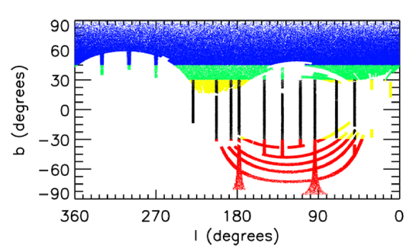
Figure 1.— The sky coverage for SDSS Data Release 7, used in this study, in Galactic coordinates. The points show a small random subsample of the full sample of 73 million stars analyzed in this paper. The different colors represent the various data file sets (blue, $\textit{b}>45^{\circ}$; green, $45^{\circ}>\textit{b}>30^{\circ}$; black, the 10 SEGUE strips; yellow, $|\textit{b}|<30^{\circ}$, stars not in SEGUE strips; and red, $\textit{b}<-30^{\circ}$).

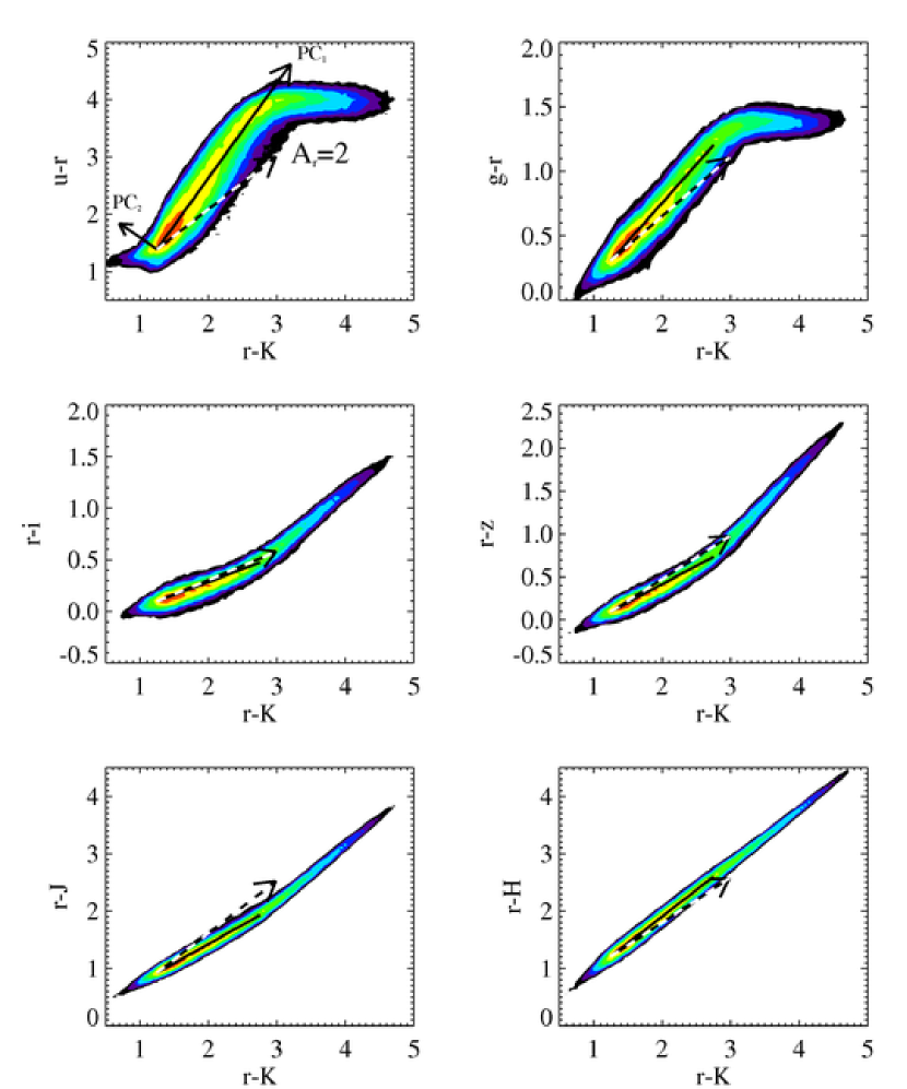
Figure 2.— The distribution of unresolved SDSS sources with 2MASS detections in the $\lambda-r$ vs. $r-K$ color-color diagrams, with $\lambda=u,g,i,z,J$ and $H$. The source density is shown as color-coded maps, and it increases from black to green to red. The two arrows marked PC₁ and PC₂ in the top left panel illustrate the “principal color” axes discussed in text and used to track the locus shifts due to interstellar dust reddening. The dashed vector in each panel shows the reddening vector for $A_{r}=2$ and standard $R_{V}=3.1$ dust (Cardelli et al., 1989).

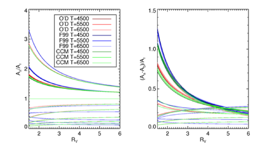
Figure 3.— Model predictions for the extinction curve shape as a function of $R_{V}$ for three different models: O’D (O’Donnell, 1994), F99 (Fitzpatrick, 1999), and CCM (Cardelli et al., 1989), evaluated for stars with three different effective temperatures (as listed in the legend, in Kelvin). The left panel shows $C_{\lambda}=A_{\lambda}/A_{r}$ for $\lambda=(u,g,r,i,z,J,H,K)$ (top to bottom, respectively); the right panel is analogous, except that the ratios based on colors ($u-g$, $g-r$, $r-i$, $i-z$, $z-J$, $J-H$, and $H-K$) are shown. As expected, most of the sensitivity to $R_{V}$ comes from the blue bands ($u$ and $g$).

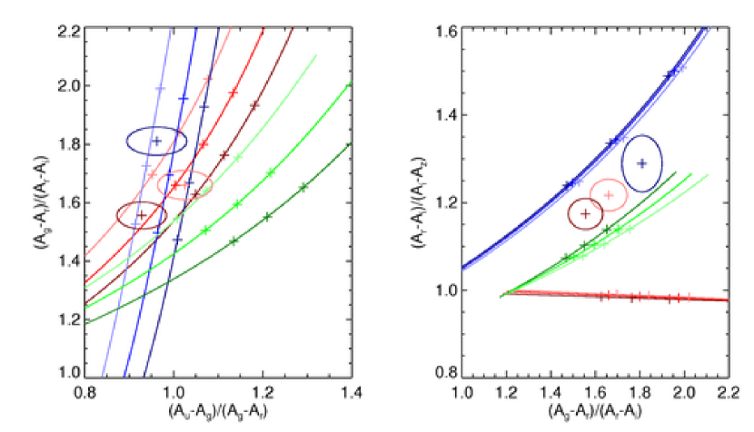
Figure 4.— A comparison of the constraints on the extinction curve shape (the three plus symbols, with approximate 1$\sigma$ uncertainty limits shown as ellipses) and three model predictions (see Figure 3 for legend; the three crosses along the curves correspond to $R_{V}$=2.6, 3.1, and 3.6). The pink symbol corresponds to the Stripe 82 region (southern Galactic hemisphere), the brown symbol to the northern Galactic hemisphere, and the blue symbol is the constraint from the Schlafly et al. (2010) analysis. The blue (Fitzpatrick, 1999) and green (Cardelli et al., 1989) models are in fair agreeement with the data, while the red model O’Donnell (1994) predicts unacceptable values of the $(A_{r}-A_{i})/(A_{i}-A_{z})$ ratio for all values of $R_{V}$ (see also Figure 5).

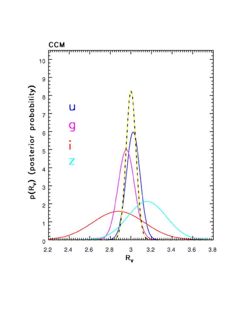
Figure 5.— Constraints on $R_{V}$ based on the CCM (Cardelli et al., 1989) dust reddening law. Only the SDSS bands, which provide the strongest constraints on $R_{V}$, are shown (see the legend). The dashed line shows the overall constraint on $R_{V}$ (posterior probability distribution for a flat prior), with the best-fit value of $R_{V}=3.01\pm 0.05$.

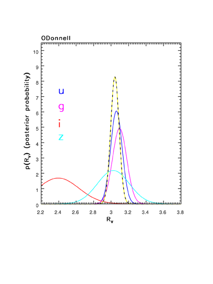
Figure 6.— Analogous to Figure 5, except that O’Donnell (1994) dust reddening law is used. The predicted extinction in the $i$ band is inconsistent with constraints from other bands.

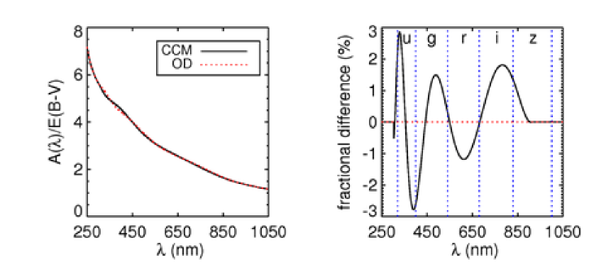
Figure 7.— The left panel shows the CCM (black, solid line) and the O’Donnell (red, dashed line) dust reddening laws as function of wavelength. The right panel displays the fractional difference between the two dust extinction models with the SDSS filter transmission regions overlaid (vertical, blue, dashed lines). Given the filter transmission regions, the largest integrated difference is expected in the $i$ band, which is what we observe.

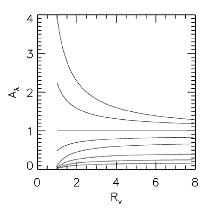
Figure 8.— The adopted $A_{\lambda}/A_{r}$ ratio, shown as a function of $R_{V}$, for $\lambda=(ugrizJHK)$, from top to bottom ($A_{r}=1$). The curves are computed for an F star using the CCM (Cardelli et al., 1989) dust reddening law.

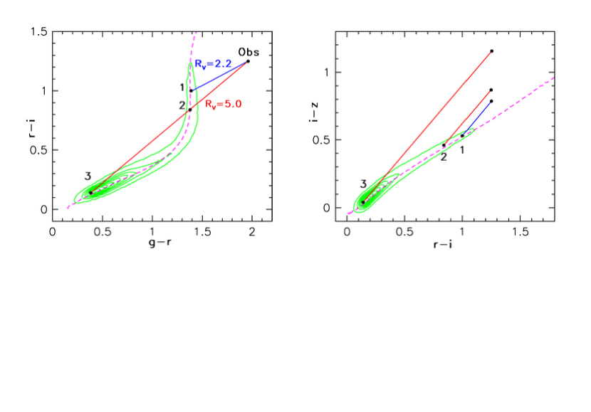
Figure 9.— An illustration of the constraints on intrinsic stellar colors, extinction in the $r$ band, $A_{r}$, and the ratio of total to selective extinction, $R_{V}$. In both diagrams, the linearly-spaced contours show the main stellar locus as observed at high Galactic latitudes. The dashed lines mark the median stellar locus from Covey et al. (2007). In the left panel, the dot marked “Obs” represents a hypothetical observation. Depending on the adopted $R_{V}$, as marked, different combinations of intrinsic stellar colors (i.e., the position along the stellar locus) and $A_{r}$ are consistent with the observed $g-r$ and $r-i$ colors. Multiple solutions are possible even for a fixed value of $R_{V}$. The three solutions marked 1-3 correspond to ($R_{V}$,$A_{r}$)= 1:(2.2,1.0), 2:(5.0,2.2), and 3:(5.0,6.0). As shown in the right panel, these degeneracies are broken if the $i-z$ color is also available: the three ($R_{V}$,$A_{r}$) combinations have different reddened $i-z$ colors which breaks the degeneracy between the intrinsic stellar color and $A_{r}$. The degeneracy is broken because the reddening vectors in the right panel are nearly parallel despite very different $R_{V}$ values.

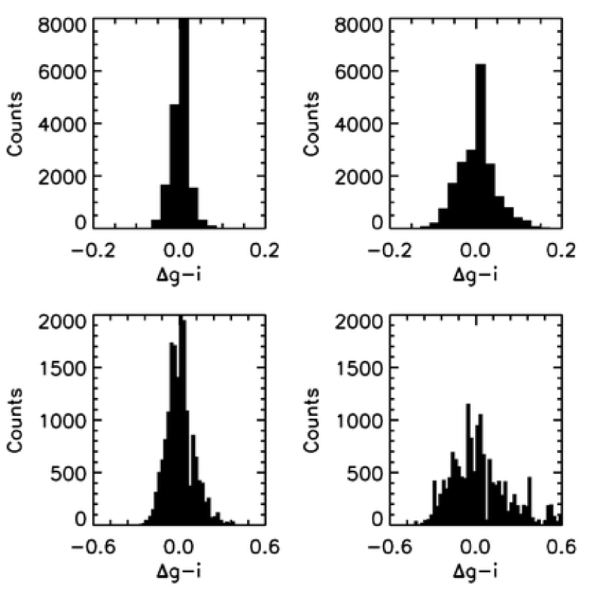
Figure 10.— A Monte Carlo study of best-fit stellar model errors (parametrized by the $g-i$ color) as a function of photometric errors, for a fiducial star with $g-i$=1.95 and $A_{r}$=1.5 (the abscissa, $\Delta$$g-i$=true - fit). The photometric errors are generated from Gaussian distributions with widths equal to 0.01 mag (top left), 0.02 mag (top right), 0.04 mag (bottom left) and 0.08 mag (bottom right). The errors in the best-fit $g-i$ are about twice as large as assumed photometric errors.

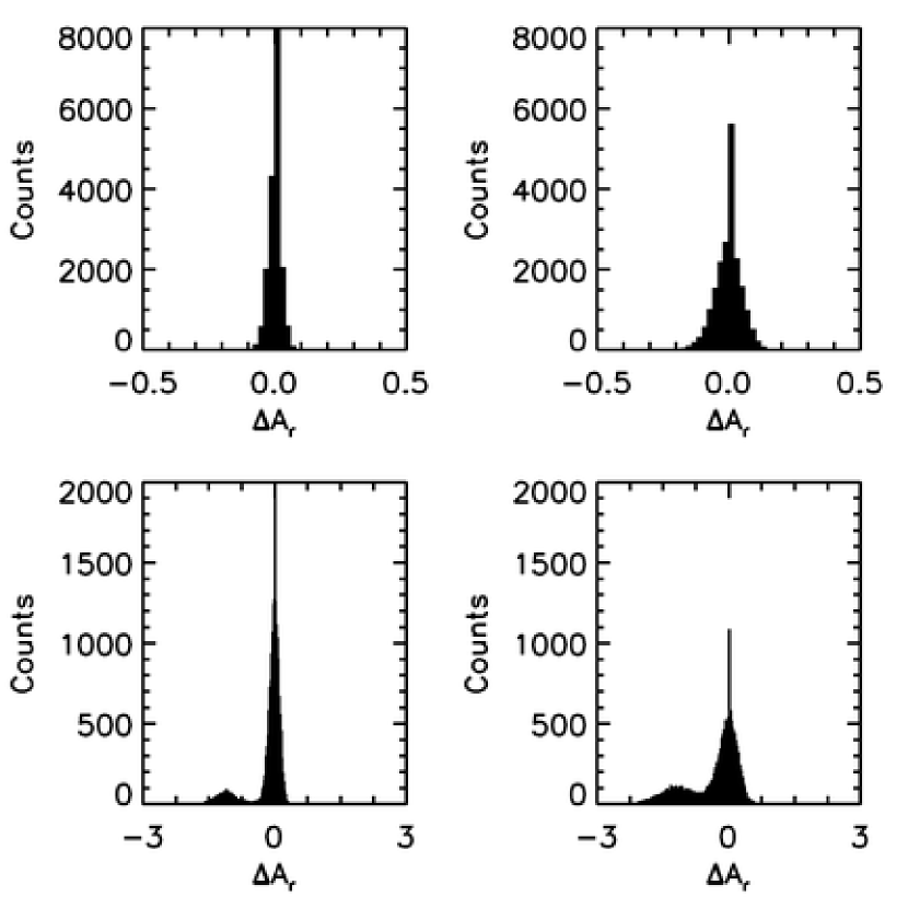
Figure 11.— Analogous to Fig. 10, except that the errors in the best-fit $A_{r}$ are shown ($\Delta$$A_{r}$)=true - fit). Note that for large photometric errors (the bottom two panels), the $A_{r}$ error distribution becomes bimodal; the additional mode corresponds to a solution with a bluer star with more reddening.

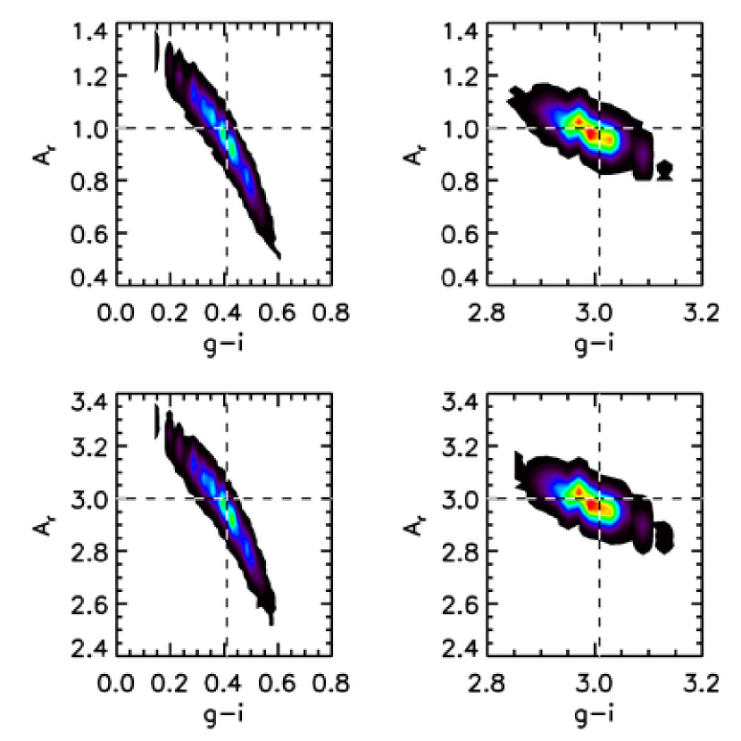
Figure 12.— Analysis of the covariance in the best-fit values for $A_{r}$ and $g-i$ using a simulated dataset. The panels show the distributions of the best-fit values for $A_{r}$ and $g-i$ for two different fiducial stars (left column: a blue star with true $g-i$=0.4; right column: a red star with true $g-i$=3.0), and two different extinction values (top panels: $A_{r}=1$; bottom panels: $A_{r}$=3). Photometric errors in the $ugriz$ bands are generated using Gaussian distributions with $\sigma$=0.02 mag (uncorrelated between different bands). Note that the $A_{r}$ vs. $g-i$ covariance is larger for the blue star, and does not strongly depend on assumed $A_{r}$.

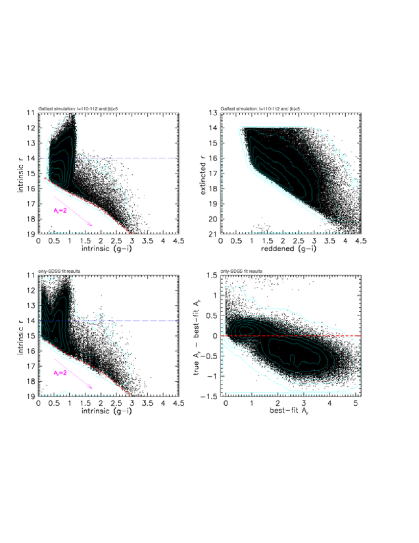
Figure 13.— Analysis of a Galfast simulated SDSS-2MASS sample from a SEGUE strip ($l\sim 110^{\circ}$ and $|b|<5^{\circ}$). The $r$ vs. $g-i$ color-magnitude diagrams in the top two panels explain why the fraction of giants is much larger than observed at high Galactic latitudes. The same simulated sample, defined by observed extincted magnitude cuts $14<r<21$ and $K<14.3$ (Vega) is shown in both panels. The left panel is constructed using un-extincted magnitudes, and the right panel with “observed” magnitudes (note the offset of the y axis by 2 mag). The horizontal dashed line in the left panel shows the SDSS saturation limit; stars above this line are dominated by red giants (the “plume” towards towards $g-i\sim 1$). The diagonal dashed line shows the magnitude limit for main sequence stars with $K<14.3$ and no dust extinction. The reddening arrow corresponds to $A_{r}=2$ and $R_{V}=3.1$ CCM extinction curve. The bottom left panel is analogous to the top left panel, except that the SDSS-based best-fit values for $g-i$ and $A_{r}$ are used. The bottom right panel shows the difference between the input value of $A_{r}$ and the best-fit values, as a function of the latter. The dashed line is added to guide the eye. The root-mean-square scatter for the $A_{r}$ difference (rms for y axis) is 0.33 mag, and the bias for large $A_{r}$ is about 15% (an overestimate of $A_{r}$ due to color-$A_{r}$ degeneracy, see text).

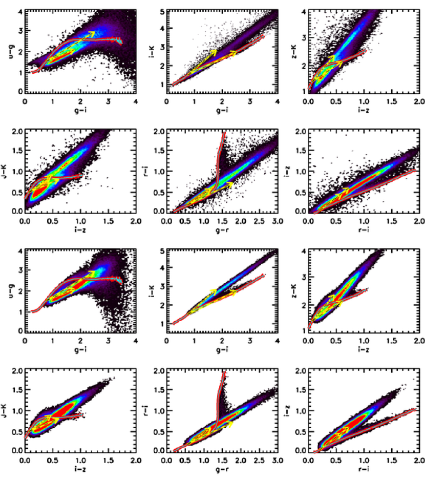
Figure 14.— A comparison of six SDSS-2MASS color-color diagrams for data from the SEGUE $l\sim 110^{\circ}$ strip (the top six panels), and for a mock catalog produced with the Galfast code (the bottom six panels). The color-coded contours shows the source counts on a linear scale. The two dashed arrows show reddening vectors for $A_{r}=2$ and $R_{V}=2$ and 4. The locus of circles shows the Covey et al. (2007) empirical SED library and illustrates the morphology of the same diagrams observed at high Galactic latitudes (and corrected using the SFD map; typically $A_{r}\sim 0.1$). The two sets of diagrams are encouragingly similar, with a few detailed differences: the observed diagrams have more outliers, and a few diagrams (e.g., $J-K$ vs. $i-z$ and $i-z$ vs. $r-i$) imply different reddening vectors than used in simulations ($R_{V}=3.1$).

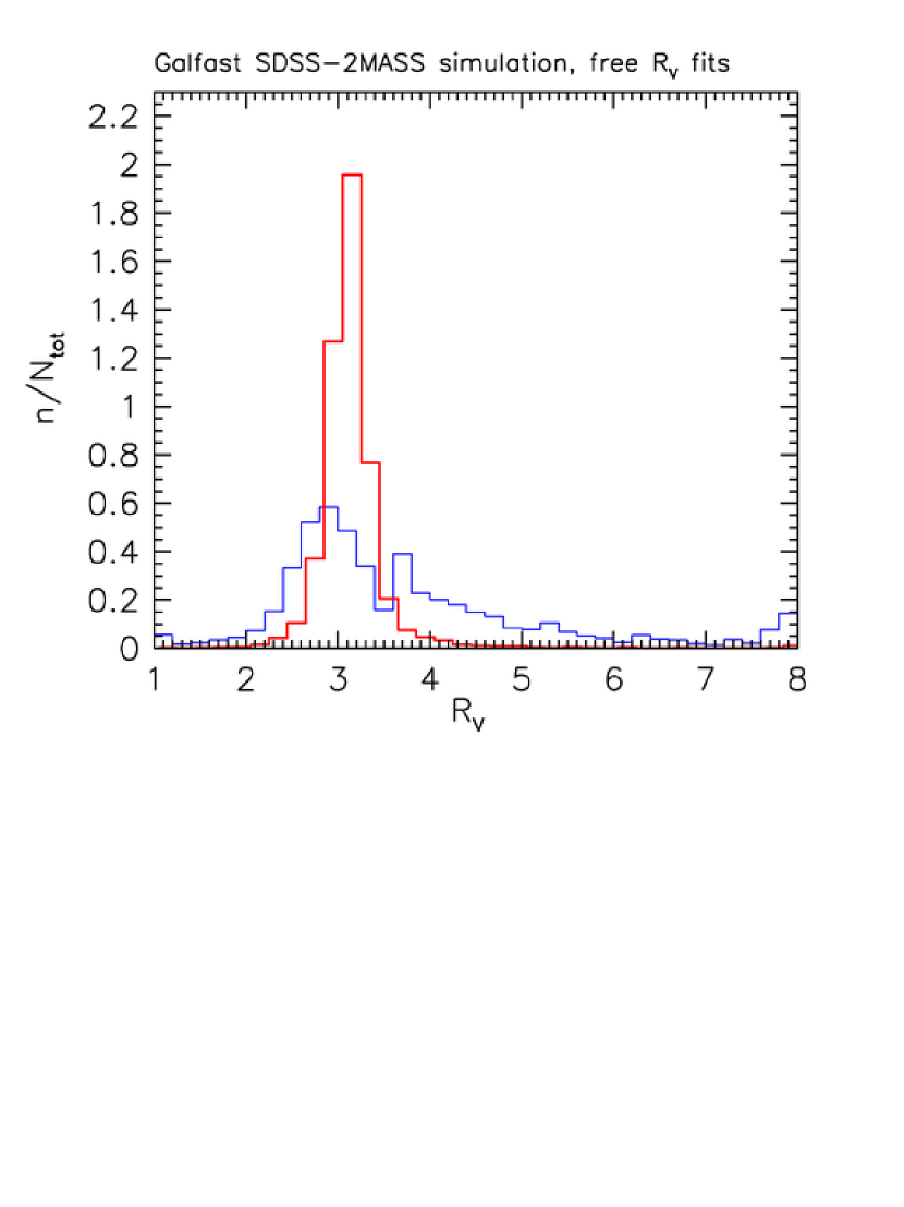
Figure 15.— A comparison of the best-fit $R_{V}$ values for SDSS-2MASS (narrow histogram) and only-SDSS (broad histogram) cases, using a simulated Galfast mock catalog. The input value is fixed to $R_{V}=3.1$. The equivalent Gaussian widths determined from the interquartile range are 0.1 and 1.2, respectively.

Figure 16.— The left panel shows the relationship between best-fit $A_{r}$ and distance computed using the SDSS-based best-fit stellar color and a photometric parallax relation appropriate for main sequence stars, for the same simulated sample as in Figures 13 and 14. The color-coded map shows the counts of stars on a linear scale. The dashed lines isolate candidate red giant stars that have small distances and large $A_{r}$. The top right panel is analogous to the top left panel, except that the best-fit values correspond to SDSS-2MASS data. The bottom left panel shows the median input absolute magnitude ($M_{r}$) for stars in each pixel, color coded according to the legend in the lower right corner. The “red giant region” in the top two panels is dominated by giants ($M_{r}<3$). The bottom right panel shows the difference between true absolute magnitude and an estimate obtained from the “dusty parallax relation” (see eq. 13), as a function of the latter. The dashed line has is added to guide the eye. The root-mean-square scatter between the two magnitudes (rms for y axis) is 1.1 mag.

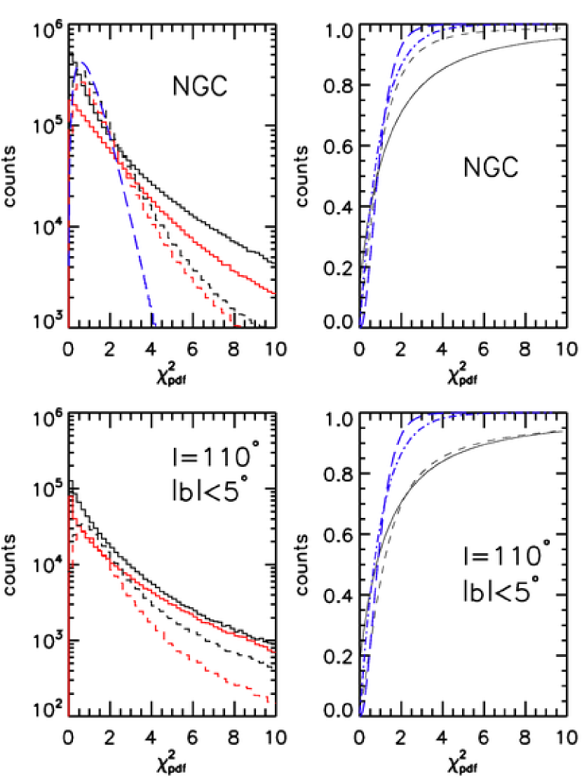
Figure 17.— The distribution of the best-fit $\chi^{2}_{\mathrm{pdf}}$ ($R_{V}=3.1$), with differential distributions in the left two panels, and cumulative distributions in the right two panels. The top two panels correspond to the north Galactic cap region ($b>45^{\circ}$) and the bottom two panels to the SEGUE $l\sim 110^{\circ}$ strip, limited to $|b|<5^{\circ}$ (a high-extinction region). The solid lines are used for SDSS-only fits, and the dashed lines for fits to SDSS-2MASS data. In the two left panels, the top solid line corresponds to subsamples of stars with $r<20$, and the bottom solid line to stars with $20<r<21$. The top dashed line corresponds to the full SDSS-2MASS sample, and the bottom dashed line to subsamples with $K<13.9$ (Vega scale, approximately corresponding to $K$ band errors up to 0.05 mag). The solid lines in the right panels correspond to the full SDSS sample, and the short-dashed lines to the full SDSS-2MASS sample. The dot-dashed and long-dashed lines correspond to $\chi^{2}_{\mathrm{pdf}}$ distributions with 2 and 5 degrees of freedom. The long-dashed line in the top left panel corresponds to the $\chi^{2}_{\mathrm{pdf}}$ distribution with 5 degrees of freedom for the full SDSS-2MASS sample.

x

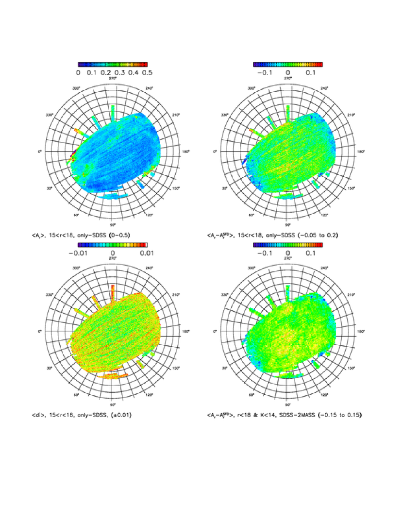
Figure 18.— Analysis of the best-fit results for $A_{r}$ in the low-extinction region with $b>30^{\circ}$. The top left panel shows the median $A_{r}$ in 0.6 deg² pixels in Lambert projection. The values are linearly color-coded according to the legend. Stars with $15<r<18$ and $\chi^{2}_{\mathrm{pdf}}<2$ from only-SDSS sample with fixed $R_{V}$ are used for the plot. The median difference between $A_{r}$ and the values given by the SFD map are shown in the top right panel. Note the striping reminiscent of the SDSS scanning pattern. The bottom left panel shows the median difference between observed and best-fit model magnitudes in the $i$ band. The bottom right panel is analogous to the top right panel, except that only the subset of stars also detected by 2MASS ($K<14$) and with full SDSS-2MASS fits (fixed $R_{V}$) are used. Note the much better agreement with the SFD values than in the top right panel. For more details, please see §3.1.2.

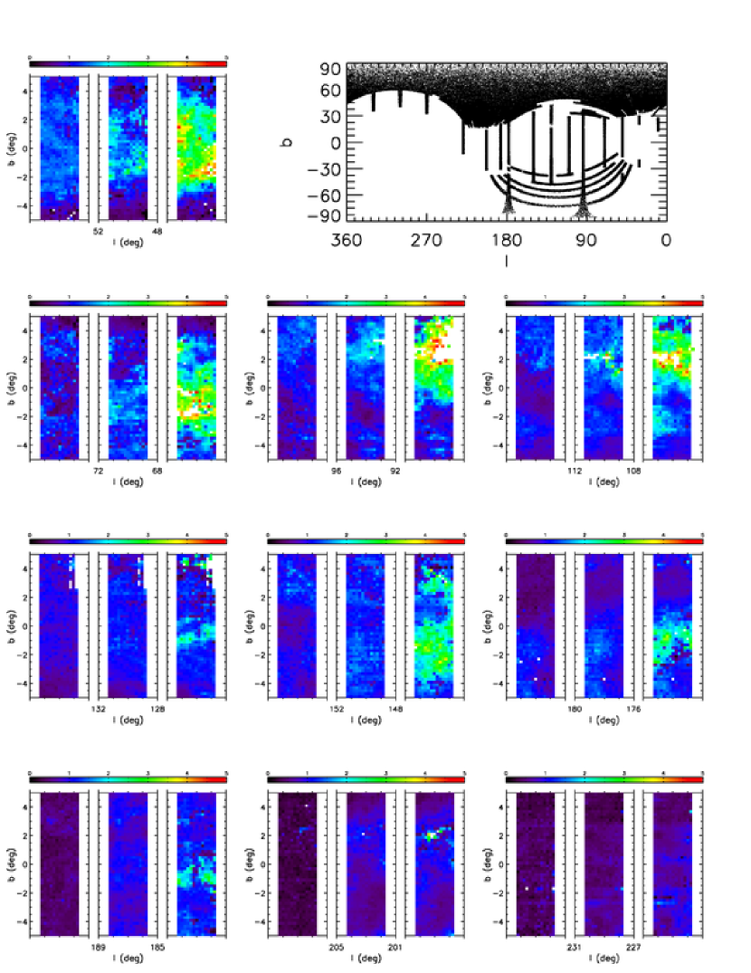
Figure 19.— The color-coded maps show the best-fit $A_{r}$ based on SDSS data for the ten analyzed SEGUE stripes. Each stripe is limited to the range of $|b|<5^{\circ}$. A fixed $R_{V}=3.1$ is assumed. The legend above each panel shows the color scale, and each 12$\times$12 arcmin² pixel shows the median $A_{r}$. For each stripe, three distance ranges are shown: 0.3-0.6 kpc (left), 1-1.5 kpc (middle) and 2-2.5 kpc (right). It is assumed that all stars are on main sequence when estimating distances. Only stars with best-fit $\chi^{2}_{pdf}<2$ and outside the red giant region (selected here by $A_{r}<1.5+1.5\,D_{\rm kpc}$) are used for the plot. The top right panel shows the sky coverage of the full analyzed dataset.

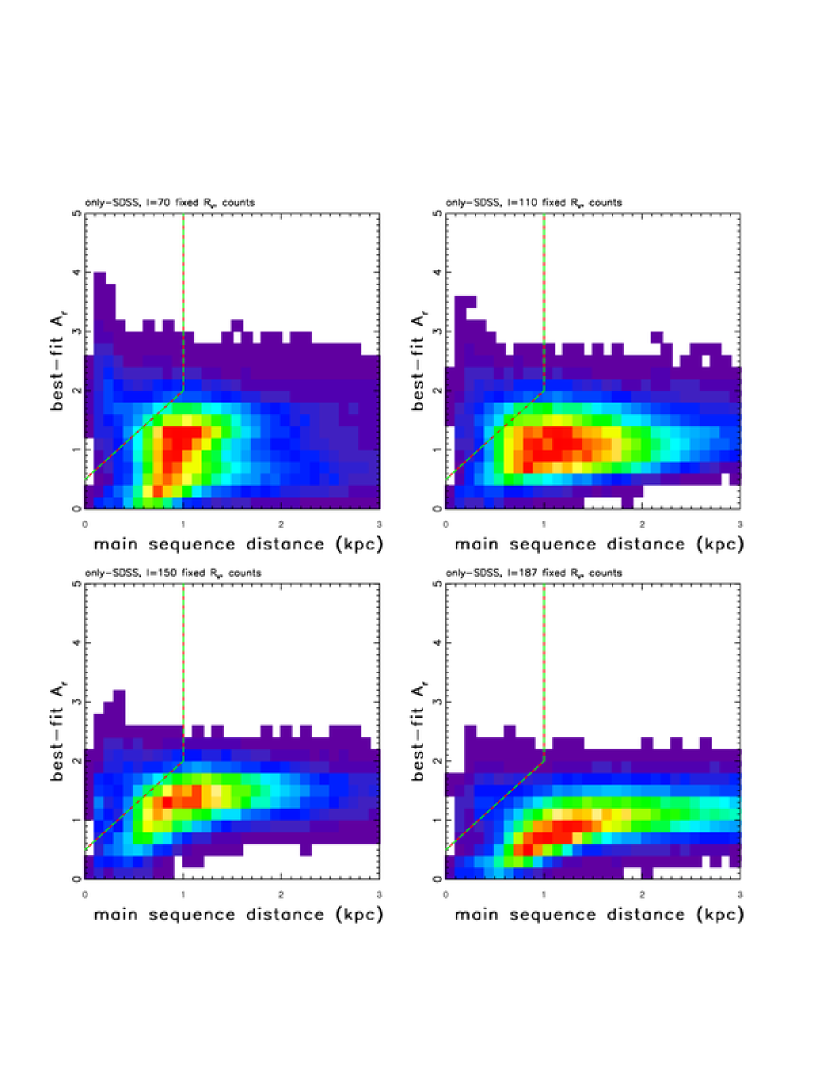
Figure 20.— The counts of stars in the only-SDSS case best-fit $A_{r}$ vs. best-fit main sequence distance diagram for four SEGUE strips (top left: $l=70^{\circ}$, top right: $l=110^{\circ}$, bottom left: $l=150^{\circ}$, bottom right: $l=187^{\circ}$; for all panels $|b|<5^{\circ}$). Only stars with $\chi^{2}_{\mathrm{pdf}}<2$, $r<19$ and error in the $u$ band below 0.05 mag are used. Counts are normalized to the maximum value and color coded on the same linear scale, from blue (low) to red (high). The two dashed lines mark a region dominated by red giant stars (the top left corner).

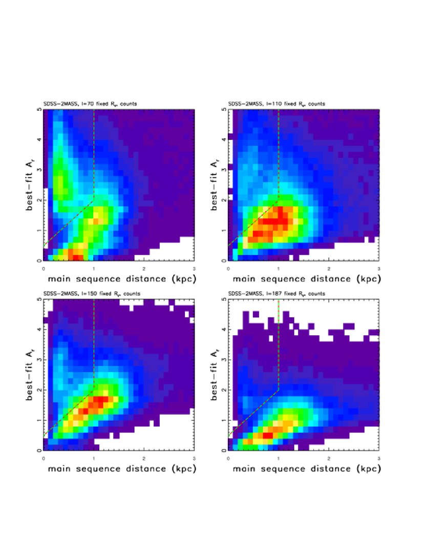
Figure 21.— Analogous to Figure 20, except for best-fits based on SDSS-2MASS sample (only stars with $\chi^{2}_{\mathrm{pdf}}<2$ and $K<15$ on Vega scale are used). Note the larger fraction of red giant stars in the top left corner, and a smaller distance limit, compared to Figure 20 and that the fraction of giants decreases with Galactic longitude.

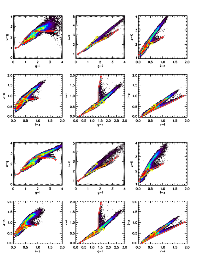
Figure 22.— A comparison of six SDSS-2MASS color-color diagrams using data from the SEGUE $l\sim 110^{\circ}$ strip (the top six panels; same as the top six panels in Figure 14, except that here only stars with $\chi^{2}_{\mathrm{pdf}}<2$ are used), and the best-fit model colors based on SDSS-2MASS dataset (the bottom six panels, in the same order). The thick lines show the Covey et al. (2007) empirical SED library and illustrate the morphology of the same diagrams observed at high Galactic latitudes. The two sets of diagrams are encouragingly similar: fits to intrinsic stellar SED and dust extinction on per star basis are capable of reproducing the morphology of observed diagrams in highly dust-extincted regions.

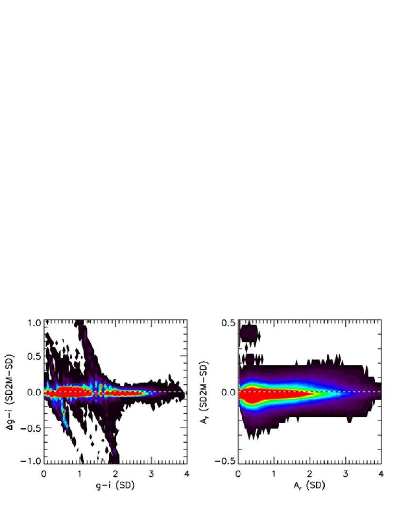
Figure 23.— A comparison of the best-fit $g-i$ (left panel) and $A_{r}$ (right panel) values obtained with a fixed $R_{V}=3.1$ for SDSS-2MASS sample from the SEGUE $l\sim 110^{\circ}$ stripe, using two different fitting methods. The abscissae show the best-fit values obtained using only-SDSS dataset (four fitted colors), and the ordinates correspond to the residuals of the SDSS-2MASS (seven fitted colors) minus the only-SDSS datasets. The number density of stars increases linearly from black to blue to red. The dashed lines are added to guide the eye.

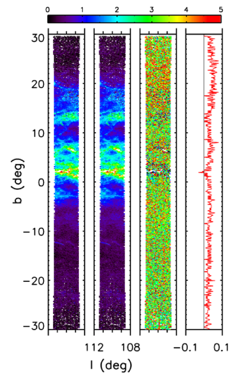
Figure 24.— Analysis of the differences in the best-fit $A_{r}$ between fits based on SDSS-2MASS dataset (first panel from the left) and those based on only-SDSS data (second panel). Only stars with best-fit $\chi^{2}_{pdf}<2$, $r<20$ and main-sequence distance $0.5-1$ kpc are used for the plot. The top legend shows the coloring code for these two panels, and each 6$\times$6 arcmin² pixel shows the median $A_{r}$ for stars with $\chi^{2}_{\mathrm{pdf}}<2$. The third panel shows the median difference between the two best-fit $A_{r}$ values (the second panel minus the first panel), with the color coding using the same palette, except that the limits are $\pm 0.1$ mag. The fourth panel shows the median difference in $A_{r}$ (i.e., the third panel) for 0.2^∘ wide bins of Galactic latitude.

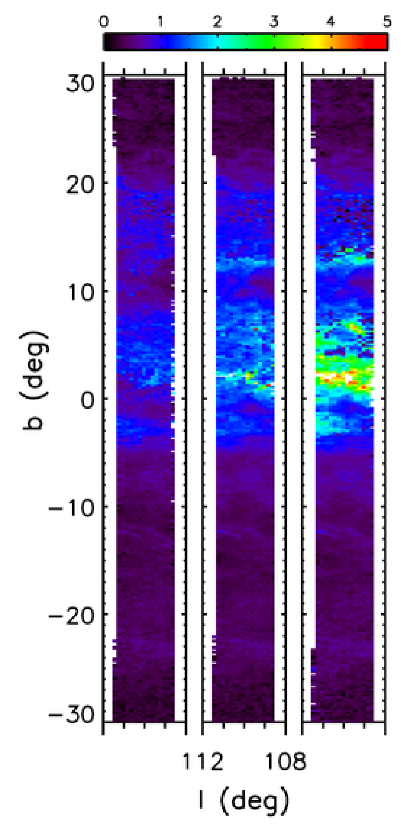
Figure 25.— The color-coded maps show the best-fit $A_{r}$ based on only-SDSS dataset for the SEGUE $l\sim 110^{\circ}$ strip. The legend shows the color scale, and each 12x12 arcmin² pixel shows the median $A_{r}$. The three panels correspond to main-sequence distance range: $0.3-0.6$ kpc (left), $1-1.5$ kpc (middle) and $2-2.5$ kpc (right). Only stars with best-fit $\chi^{2}_{pdf}<2$ and outside the red giant region (selected here by $A_{r}<1.5+1.5\,D_{\rm kpc}$) are used for the plot.

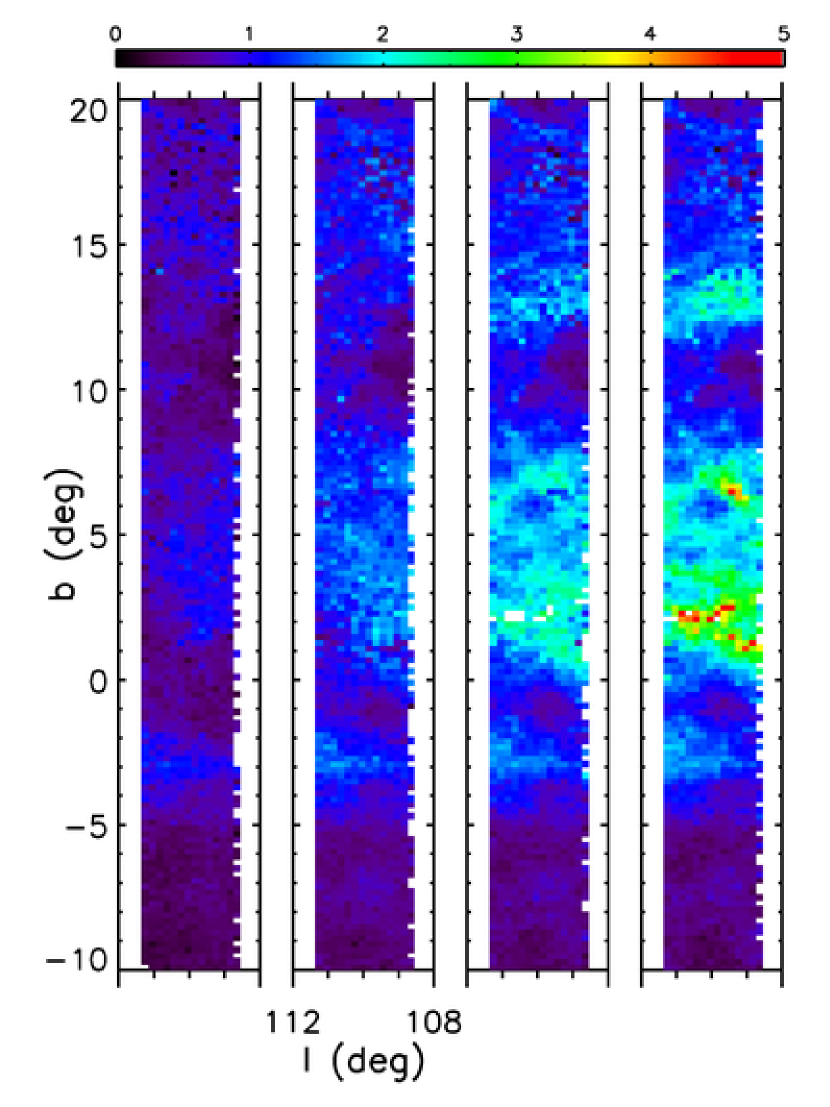
Figure 26.— Analogous to Figure 25, except using the SDSS-2MASS dataset and different distance slices (left to right: $0.1-0.5$ kpc, $0.5-0.7$ kpc, $0.7-0.9$ kpc, $0.9-1.1$ kpc). Note the abrupt increase in $A_{r}$ for stars towards $b\sim+2^{\circ}$ that are more distant than 0.9 kpc.

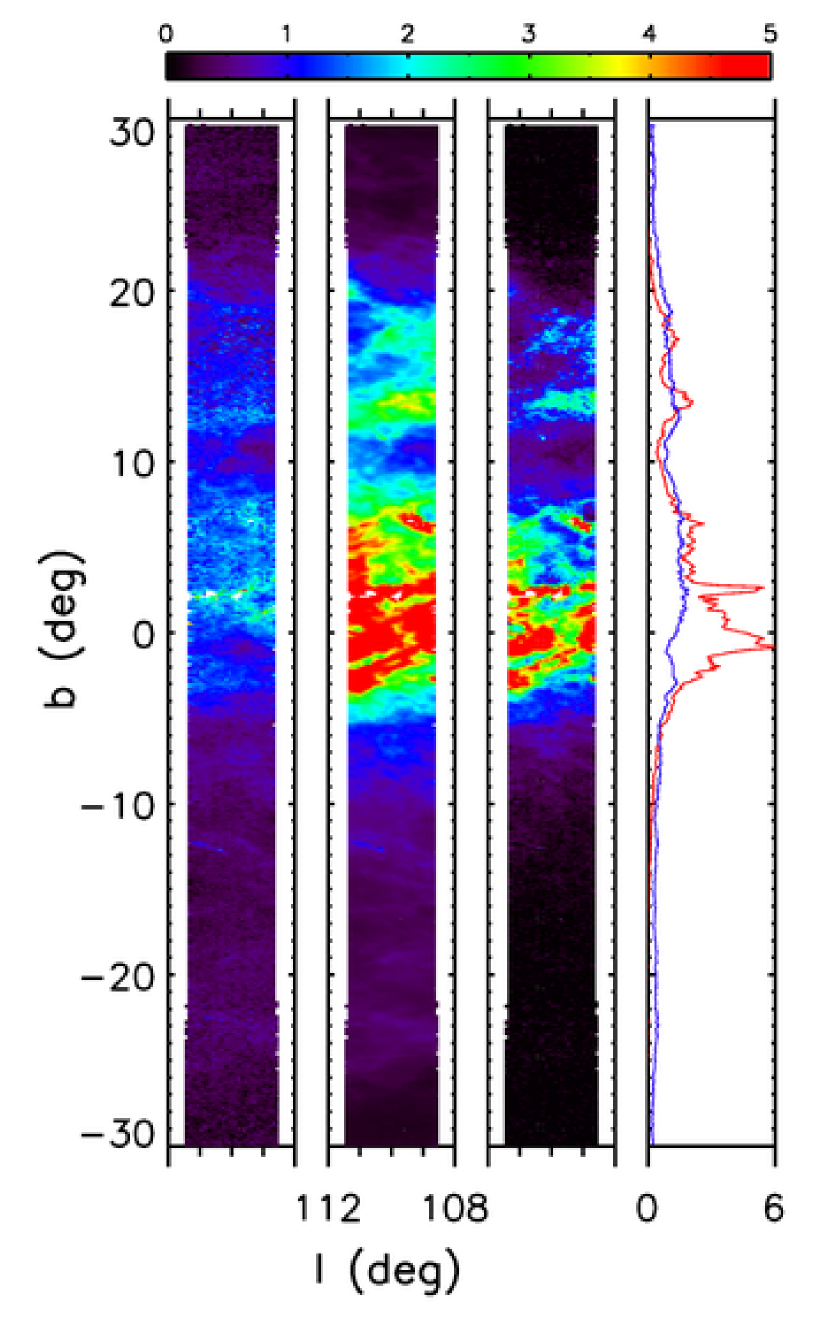
Figure 27.— Analysis of the differences between best-fit $A_{r}$ values (left panel, based on only-SDSS data; SDSS-2MASS version looks similar) and the SFD values (second panel) for stars with $\chi^{2}_{pdf}<2$ and main-sequence distance in the range $0.8-1.2$ kpc. The third panel shows the difference of the two $A_{r}$ values (the second panel minus the first panel). Each 6$\times$6 arcmin² pixel in the first three panels is color coded according to the top legend. The fourth panel shows the median best-fit $A_{r}$ (blue line) and the median SFD value (red line) for 0.2^∘ wide bins of Galactic latitude. If the SFD maps are correct, then the dust structures discernible in the two right panels at $b\sim 0^{\circ}$ and $b\sim+2^{\circ}$ must be more distant than $\sim$1 kpc. This conclusion is independently confirmed for the latter dust cloud in Figure 26.

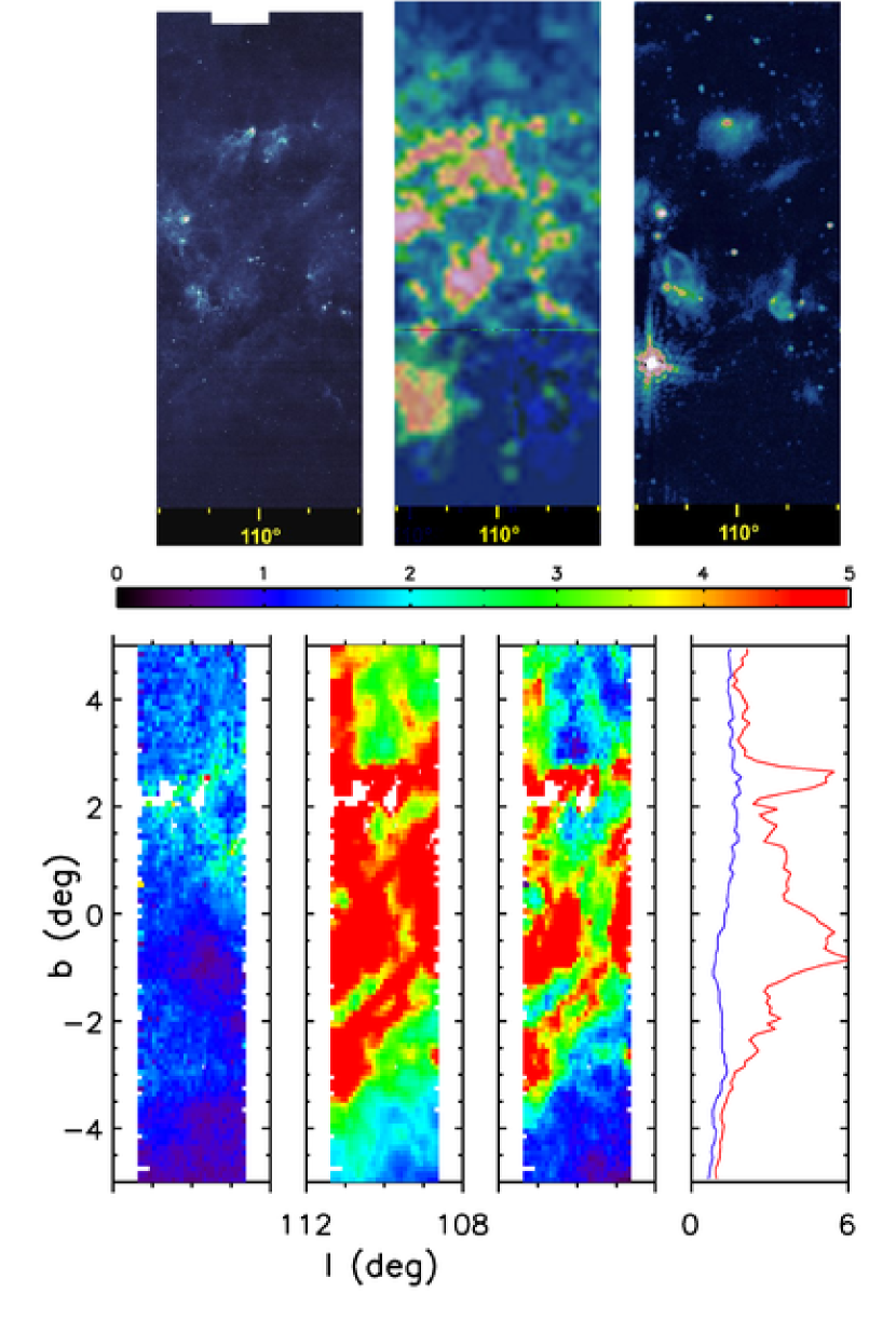
Figure 28.— The bottom four panels show the $|b|<5^{\circ}$ subregion of the panels shown in Fig. 27. The top three panels show the mid-IR (left), CO (middle) and radio continuum (right) maps on approximately the same scale (obtained using “The Milky Way Explorer” by Kevin Jardine). The few small irregular white regions in the bottom three maps do not contain any stars with good photometry. Assuming that the SFD map is not grossly incorrect, the dust extinction determined here implies that most of the molecular cloud structures seen in the top middle panel must be more distant than $\sim$1 kpc.

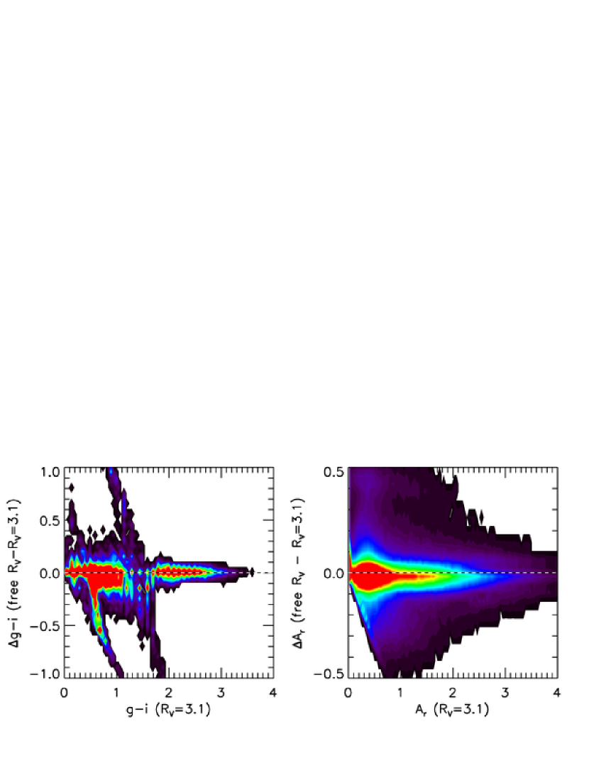
Figure 29.— A comparison of the best-fit $g-i$ (left panel) and $A_{r}$ (right panel) values for two different treatments of $R_{V}$, for stars in the $l=110^{\circ}$ SEGUE strip (using SDSS-2MASS data). Only stars with best-fit $\chi^{2}_{pdf}<2$, $r<20$ and $K<13.9$ (Vega) are used for the plot. The abscissae show the best-fit values obtained for a fixed $R_{V}=3.1$ and the ordinates correspond to the residuals of the differences in the best-fit values when $R_{V}$ is treated as a free-fitting parameter (“free $R_{V}$” $-$ “$R_{V}$=3.1”). The number density of stars increases from black to blue to red. The dashed lines are added to guide the eye.

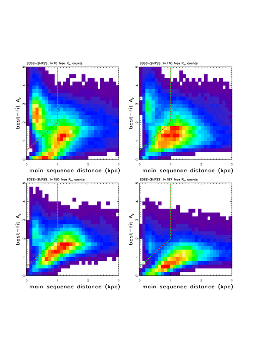
Figure 30.— The $A_{r}$ map analogous to Figure 21, except that $R_{V}$ is treated as a free parameter. Only stars with $|b|<5^{\circ}$, $\chi^{2}_{\mathrm{pdf}}<2$, $r<19$, and $K<15$ (on Vega scale) are used.

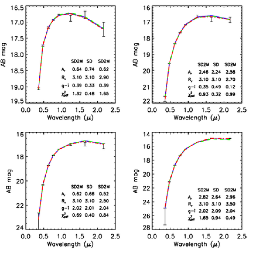
Figure 31.— A comparison of three different types of best-fit SEDs: using only SDSS data with fixed $R_{V}=3.1$ (blue line), and using joint SDSS-2MASS dataset with fixed $R_{V}$ (green line) and with free $R_{V}$ (red line). As demonstrated by the similarity of best-fit lines, the differences in best-fit parameters, listed in each panel, are due to degeneracies between intrinsic stellar color, amount of dust and $R_{V}$. The shown cases correspond to blue and red stars (top row vs. bottom row), and small and large $A_{r}$ (left column vs. right column).

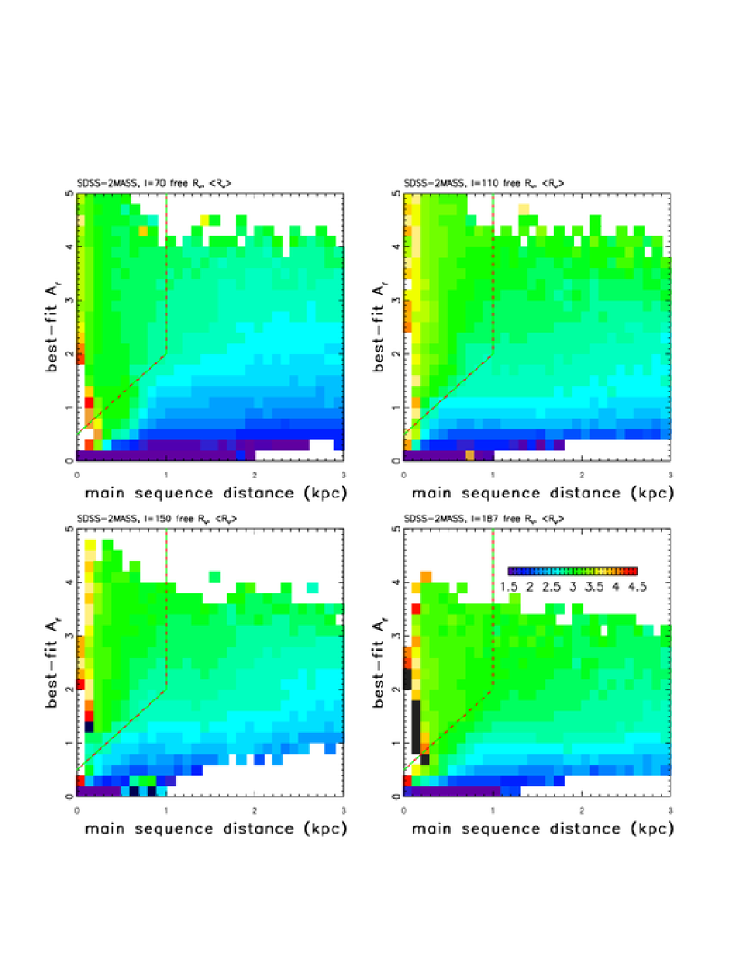
Figure 32.— Similar to Figure 21, except that $R_{V}$ is treated as a free parameter, and the color-coded map shows the median value of $R_{V}$ (ranging from blue for $R_{V}=1.5$ to red for $R_{V}=4.5$, green corresponds to $R_{V}=3$; see the legend in the bottom right panel). Only stars with $|b|<5^{\circ}$, $\chi^{2}_{\mathrm{pdf}}<2$, $r<19$, and $K<15$ (on Vega scale) are used. Note that red giant stars (top left corner) have consistently larger values of $R_{V}$, and that consistently $R_{V}<3$ when $A_{r}<1$ for main sequence stars. In other regions in this diagram where $R_{V}$ is determined robustly, $R_{V}=3.1$ cannot be ruled out in any of the ten SEGUE stripes at a precision level of $\sim 0.1-0.2$.

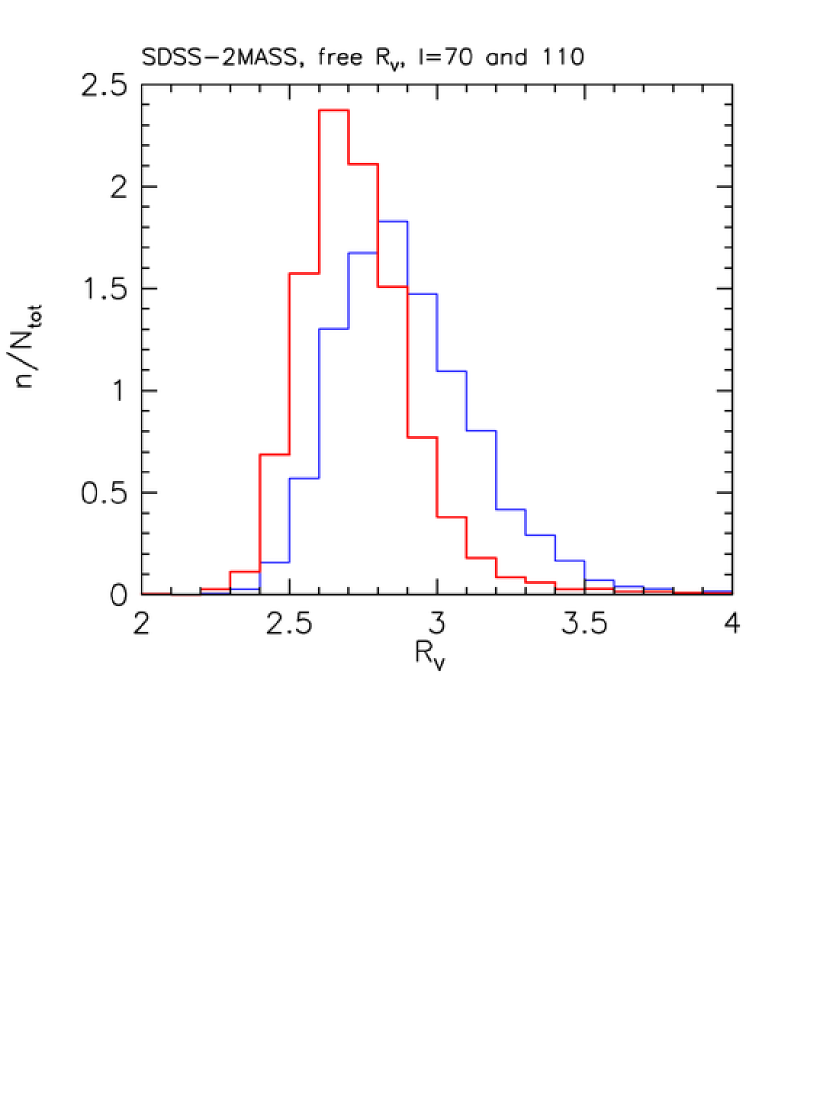
Figure 33.— A comparison of the best-fit $R_{V}$ values for SDSS-2MASS free-$R_{V}$ case and stars with distances in the 1.0-2.5 kpc range and $A_{r}>2.5$, selected from $l=70^{\circ}$ (red, left histogram) and $l=110^{\circ}$ (blue, right histogram) stripes (other selection criteria are the same as for stars plotted in Figure 32).

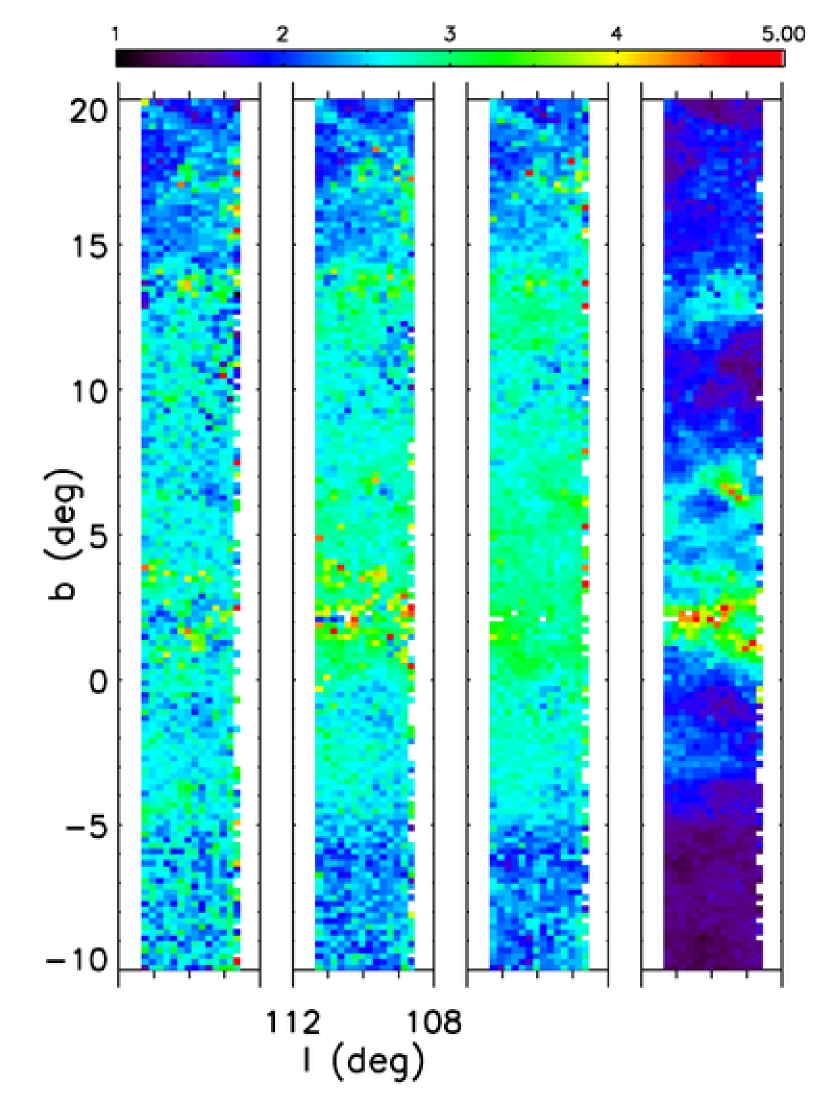
Figure 34.— The first three panels show the median $R_{V}$ obtained using SDSS-2MASS sample for the SEGUE $l=110^{\circ}$ strip, and for distance range $0.5-0.7$ kpc (first), $0.7-0.9$ kpc (second), and $0.9-1.1$ kpc (third). Only stars outside the “red giant” region, see Figure 21, and with $\chi^{2}_{pdf}<2$, $r<21$ and $K<14.3$ (Vega) are used for the plot. The pixel size is 6$\times$6 arcmin², and the $R_{V}$ coloring scheme is shown at the top. The fourth panel shows for reference the best-fit $A_{r}$, for the distance slice $0.9-1.1$ kpc. Note that $R_{V}$ is not reliable for $A_{r}<2$ (black and blue regions in the fourth panel).

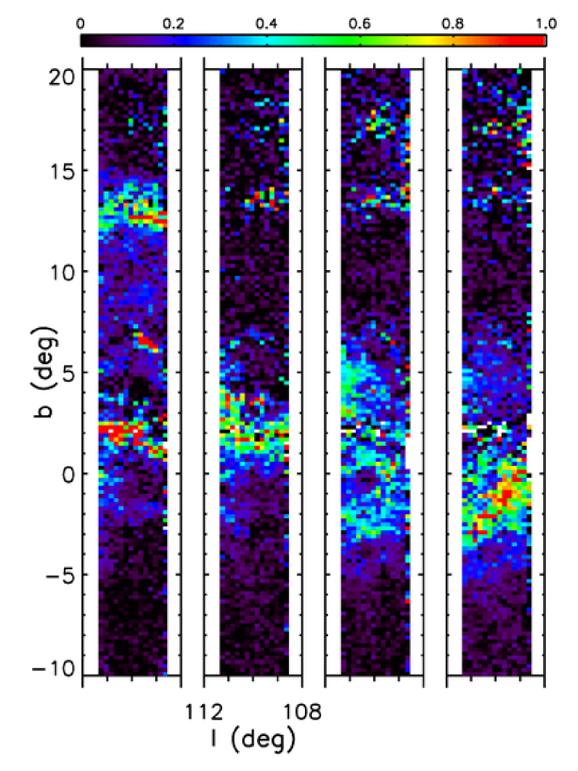
Figure 35.— Illustration of the three-dimensional dust distribution for SEGUE stripe $l\sim 110^{\circ}$ at mean distances of 1.0, 1.5, 2.0 and 2.5 kpc, using only-SDSS sample and fixed-$R_{V}$ fits. Unlike other figures that show the median $A_{r}$ along the line of sight, this figure shows the differences in the median $A_{r}$ (per 12$\times$12 arcmin² pixel) for samples at distances between the quoted distance and limiting distances 0.5 kpc larger and smaller than the mean distance (e.g., the first panel shows the difference between the median $A_{r}$ for 0.5-1.0 kpc and 1.0-1.5 kpc subsamples). It is easily discernible that the dust structures observed at $b\sim 2^{\circ}$ and $b\sim 13^{\circ}$ are confined to 1-1.5 kpc distance range, while the structure seen at $-3^{\circ}<b<0^{\circ}$ is due to dust at a distance of $\sim 2.5$ kpc (an analogous panel for a mean distance of 3.0 kpc shows that this structure is mostly confined to smaller distances). Note that the linear extent perpendicular to the line of sight of a given angular size is 2.5 times larger in the last than in the first panel.

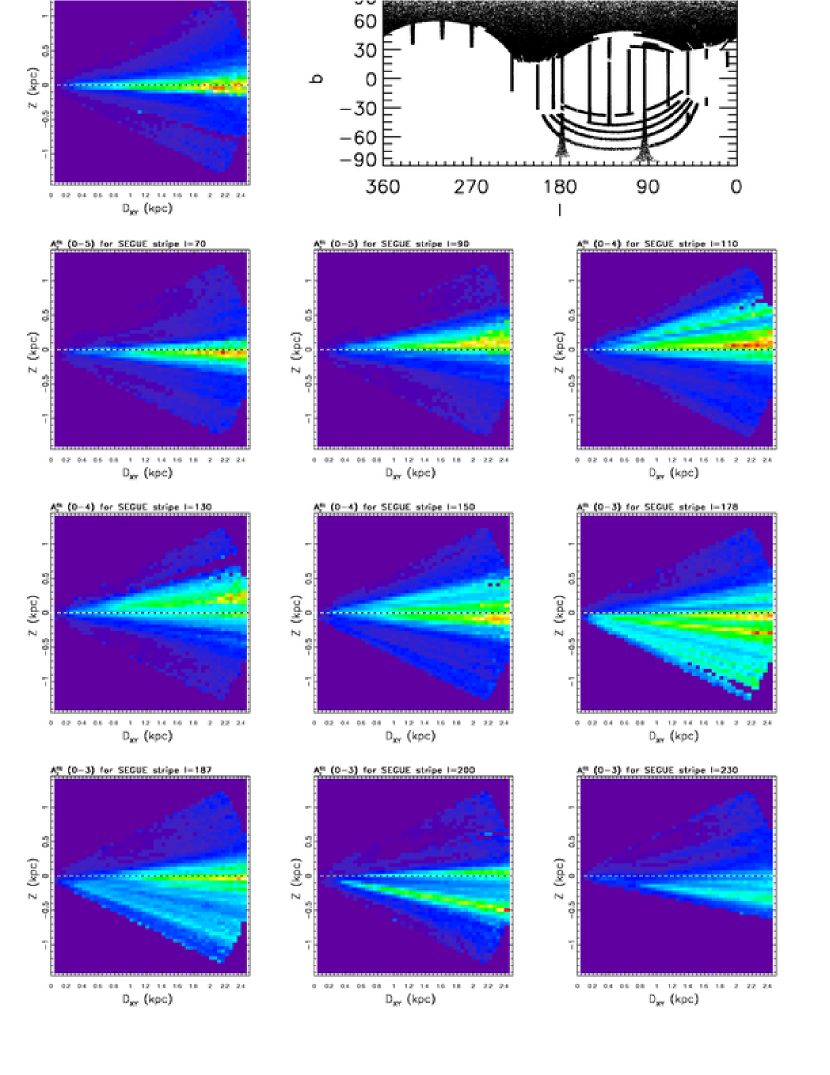
Figure 36.— The median best-fit $A_{r}$ (extinction along the line of sight) is shown as a function of distance from the Galactic plane, $Z$, and distance along the plane, $D_{xy}$, for 10 SEGUE stripes (this is not a cross-section of three-dimensional dust distribution!). The best-fit $A_{r}$ are based on the SDSS-2MASS dataset and fixed-$R_{V}$ fitting case, for stars with $\chi^{2}_{pdf}<2$ and $K<15$ (Vega). Each pixel is 50$\times$50 pc² and subtends 2.5 deg wide stripe in the perpendicular (longitude) direction. The color scheme increases linearly from blue to red with a varying maximum value: 5 for the first three panels, 4 for the next three, and 3 for the last four panels.

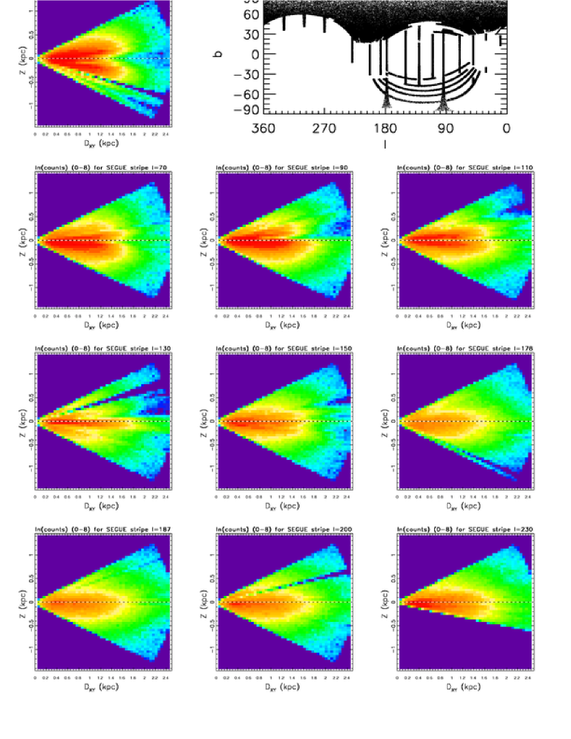
Figure 37.— The local volume number density of stars is shown as a function of distance from the Galactic plane, $Z$, and distance along the plane, $D_{xy}$, for the same samples as shown in Figure 36. The color scheme shows the counts on log scale with the same arbitrary normalization for all stripes. The fall-off of the stellar volume number density at distances beyond $\sim$1 kpc is due to the stellar color-dependent sample distance limit and does not reflect the disk structure. Note the variation of counts with Galactic longitude (the top four panels are closer to the Galactic center and contain more stars per unit volume).

References

- Abazajian et al. (2009) Abazajian, K. N., Adelman-McCarthy, J. K., Agüeros, M. A., et al. 2009, ApJS, 182, 543
- Amôres & Lépine (2005) Amôres, E. B. & Lépine, J. R. D. 2005, AJ, 130, 659
- Arce & Goodman (1999) Arce, H. G. & Goodman, A. A. 1999, ApJ, 512, L135
- Bailer-Jones (2011) Bailer-Jones, C. A. L. 2011, MNRAS, 411, 435
- Bond et al. (2010) Bond, N. A., Ivezić, Ž., Sesar, B., et al. 2010, ApJ, 716, 1
- Cardelli et al. (1989) Cardelli, J. A., Clayton, G. C., & Mathis, J. S. 1989, ApJ, 345, 245
- Covey et al. (2007) Covey, K. R., Ivezić, Ž., Schlegel, D., Finkbeiner, D., et al. 2007, AJ, 134, 2398
- Draine (2011) Draine, B. T. 2011, Physics of the Interstellar and Intergalactic Medium, ed. Draine, B. T.
- Eisenstein et al. (2006) Eisenstein, D. J., Liebert, J., Harris, H., et al. 2006, ApJS, 167, 40
- Finlator et al. (2000) Finlator, K., Ivezić, Ž., Fan, X., Strauss, M. A., et al. 2000, AJ, 120, 2615
- Fitzpatrick (1999) Fitzpatrick, E. L. 1999, PASP, 111, 63
- Fitzpatrick & Massa (2009) Fitzpatrick, E. L. & Massa, D. 2009, ApJ, 699, 1209
- Flaugher (2008) Flaugher, B. 2008, in A Decade of Dark Energy: Spring Symposium, Proceedings of the conferences held May 5-8, 2008 in Baltimore, Maryland. (USA). Edited by Norbert Pirzkal and Henry Ferguson. http://www.stsci.edu/institute/conference/spring2008
- Fukugita et al. (1996) Fukugita, M., Ichikawa, T., Gunn, J. E., et al. 1996, AJ, 111, 1748
- Girardi et al. (2005) Girardi, L., Groenewegen, M. A. T., Hatziminaoglou, E., & da Costa, L. 2005, A&A, 436, 895
- Gorbikov & Brosch (2010) Gorbikov, E. & Brosch, N. 2010, MNRAS, 401, 231
- Gunn et al. (1998) Gunn, J. E., Carr, M., Rockosi, C., et al. 1998, AJ, 116, 3040
- Gunn et al. (2006) Gunn, J. E., Siegmund, W. A., Mannery, E., et al. 2006, AJ, 131, 2332
- Helmi et al. (2003) Helmi, A., Ivezić, Ž., Prada, F., et al. 2003, ApJ, 586, 195
- High et al. (2009) High, F. W., Stubbs, C. W., Rest, A., Stalder, B., & Challis, P. 2009, AJ, 138, 110
- Hogg et al. (2001) Hogg, D. W., Finkbeiner, D. P., Schlegel, D. J., & Gunn, J. E. 2001, AJ, 122, 2129
- Ivezić et al. (2004) Ivezić, Ž., Lupton, R. H., Schlegel, D. J., et al. 2004, Astronomische Nachrichten, 325, 583
- Ivezić et al. (2008a) Ivezić, Ž., Sesar, B., Jurić, M., et al. 2008a, ApJ, 684, 287
- Ivezić et al. (2007) Ivezić, Ž., Smith, J. A., Miknaitis, G., Lin, H., et al. 2007, AJ, 134, 973
- Ivezić et al. (2008b) Ivezić, Ž., Tyson, J. A., Acosta, E., et al. 2008b, arXiv:0805.2366
- Jones et al. (2011) Jones, D. O., West, A. A., & Foster, J. B. 2011, AJ, 142, 44
- Jurić et al. (2008) Jurić, M., Ivezić, Ž., Brooks, A., et al. 2008, ApJ, 673, 864
- Kaiser et al. (2002) Kaiser, N., Aussel, H., Burke, B. E., et al. 2002, in Society of Photo-Optical Instrumentation Engineers (SPIE) Conference Series, Vol. 4836, Society of Photo-Optical Instrumentation Engineers (SPIE) Conference Series, ed. J. A. Tyson & S. Wolff, 154–164
- Knapp & Kerr (1974) Knapp, G. R. & Kerr, F. J. 1974, A&A, 35, 361
- Lombardi & Alves (2001) Lombardi, M. & Alves, J. 2001, A&A, 377, 1023
- Lombardi et al. (2011) Lombardi, M., Alves, J., & Lada, C. J. 2011, A&A, 535, A16
- Lupton et al. (2001) Lupton, R., Gunn, J. E., Ivezić, Z., Knapp, G. R., et al. 2001, in Astronomical Society of the Pacific Conference Series, Vol. 238, Astronomical Data Analysis Software and Systems X, ed. F. R. Harnden Jr., F. A. Primini, & H. E. Payne, 269–+
- Magnier et al. (2010) Magnier, E. A., Liu, M., Goldman, B., Monet, D. G., Chambers, K. C., & Kaiser, N. 2010, Highlights of Astronomy, 15, 818
- Majewski et al. (2011) Majewski, S. R., Zasowski, G., & Nidever, D. L. 2011, ApJ, 739, 25
- McGurk et al. (2010) McGurk, R. C., Kimball, A. E., & Ivezić, Ž. 2010, AJ, 139, 1261
- Meyer et al. (2005) Meyer, J. M., Ivezić, Ž., Finkbeiner, D. P., et al. 2005, in Bulletin of the American Astronomical Society, Vol. 37, American Astronomical Society Meeting Abstracts, 131.01
- O’Donnell (1994) O’Donnell, J. E. 1994, ApJ, 422, 158
- Padmanabhan et al. (2008) Padmanabhan, N., Schlegel, D. J., Finkbeiner, D. P., et al. 2008, ApJ, 674, 1217
- Peek & Graves (2010) Peek, J. E. G. & Graves, G. J. 2010, ApJ, 719, 415
- Pier et al. (2003) Pier, J. R., Munn, J. A., Hindsley, R. B., et al. 2003, AJ, 125, 1559
- Richards et al. (2001) Richards, G. T., Fan, X., Schneider, D. P., et al. 2001, AJ, 121, 2308
- Robin et al. (2003) Robin, A. C., Reylé, C., Derrière, S., & Picaud, S. 2003, A&A, 409, 523
- Sale et al. (2009) Sale, S. E., Drew, J. E., Unruh, Y. C., Irwin, M. J., Knigge, C., Phillipps, S., Zijlstra, A. A., Gänsicke, B. T., Greimel, R., Groot, P. J., Mampaso, A., Morris, R. A. H., Napiwotzki, R., Steeghs, D., & Walton, N. A. 2009, MNRAS, 392, 497
- Schlafly & Finkbeiner (2010) Schlafly, E. F. & Finkbeiner, D. P. 2010, ArXiv e-prints
- Schlafly et al. (2010) Schlafly, E. F., Finkbeiner, D. P., Schlegel, D. J., et al. 2010, ApJ, 725, 1175
- Schlegel et al. (1998) Schlegel, D. J., Finkbeiner, D. P., & Davis, M. 1998, ApJ, 500, 525
- Sesar et al. (2008) Sesar, B., Ivezić, Ž., & Jurić, M. 2008, ApJ, 689, 1244
- Sesar et al. (2007) Sesar, B., Ivezić, Ž., Lupton, R. H., Jurić, M., et al. 2007, AJ, 134, 2236
- Skrutskie et al. (1997) Skrutskie, M. F., Schneider, S. E., Stiening, R., Strom, S. E., et al. 1997, in Astrophysics and Space Science Library, Vol. 210, The Impact of Large Scale Near-IR Sky Surveys, ed. F. Garzon, N. Epchtein, A. Omont, B. Burton, & P. Persi, 25–+
- Smith et al. (2002) Smith, J. A., Tucker, D. L., Kent, S., et al. 2002, AJ, 123, 2121
- Smolčić et al. (2004) Smolčić, V., Ivezić, Ž., Knapp, G. R., et al. 2004, ApJ, 615, L141
- Stoughton et al. (2002) Stoughton, C., Lupton, R. H., Bernardi, M., et al. 2002, AJ, 123, 485
- Tucker et al. (2006) Tucker, D. L., Kent, S., Richmond, M. W., et al. 2006, Astronomische Nachrichten, 327, 821
- Wright et al. (2010) Wright, E. L., Eisenhardt, P. R. M., Mainzer, A. K., et al. 2010, AJ, 140, 1868
- Yanny et al. (2009) Yanny, B., Rockosi, C., Newberg, H. J., et al. 2009, AJ, 137, 4377
- Yasuda et al. (2007) Yasuda, N., Fukugita, M., & Schneider, D. P. 2007, AJ, 134, 698
- York et al. (2000) York, D. G., Adelman, J., Anderson, J. E., et al. 2000, AJ, 120, 1579