Description of the Totem experimental data on elastic $pp$-scattering at $\sqrt{s}=7$ TeV in the framework of unified systematic of elastic scattering data

V. Uzhinsky^, A. Galoyan

An unified systematic of elastic (anti)proton-proton scattering data is proposed based on a simple expression for the process amplitude – $f(q)=A\ [(\pi dq)/sh(\pi dq)][i\ J_{1}(Rq)/(Rq)+\rho J_{0}(Rq)+...]$. The parameters $R$ and $d$ are obtained at a fitting of (anti)proton-proton experimental data on differential cross sections from $P_{lab}\sim$ 1 GeV/c up to Tevatron energies. The fitting gives extra-ordinary good results, $\chi^{2}/NoF\sim$ 1 of below at $|t|<$ 1.75 (GeV/c)². An extrapolation of the parameter’s energy dependencies to the LHC energies allows a good description of the Totem data up to the second diffraction maximum. Predictions for other LHC energies are presented also.

The amplitude provides one with parameterizations of total and elastic cross sections. Its impact parameter representation corresponds to the 2-dimensional Fermi-function – $1/[1+exp((b-R)/d)]$, which is very useful for Glauber calculations of nucleus-nucleus cross sections at super high energies.

It is shown for the first time that experimental high $|t|$ elastic scattering data have a weak energy dependency. This allows to describe high $|t|$ tail of the Totem data.

Introduction

According to the experimental data on elastic (anti)proton-proton scattering data in the Coulomb-nuclear interference region, the nuclear elastic scattering amplitude in the momentum representation, $f(\vec{q})$, has a small real part and a large imaginary one. Correspondingly, the amplitude in the impact parameter representation, $\gamma(\vec{b})$, has a large real part and a small imaginary one. The amplitudes are connected by the Fourier-Bessel transform:

$$f(\vec{q})=\frac{i}{2\pi}\int\ e^{i\ \vec{q}\vec{b}}\gamma(\vec{b})d^{2}b=i\int^{\infty}_{0}b\ J_{0}(\vec{q}\vec{b})\ \gamma(\vec{b})db,$$ (1)

$$\gamma(\vec{b})=\frac{1}{2\pi i}\int\ e^{i\vec{q}\vec{b}}f(\vec{q})d^{2}q=\frac{1}{i}\int^{\infty}_{0}\ q\ J_{0}(\vec{q}\vec{b})\ f(\vec{q})dq,$$ (2)

$$\sigma^{tot}=4\pi\ Imf(0)=4\pi\ \int^{\infty}_{0}b\ Re\ \gamma(b)db,$$ (3)

$$\sigma^{el}=2\pi\int^{\infty}_{0}b\ |\gamma(b)|^{2}db,$$ (4)

$$d^{2}\sigma/dq^{2}=|f(\vec{q})|^{2},\ \ \ Ref(0)\sim 0\ \ \ Im\gamma(b)\sim 0,$$ (5)

where $\vec{q}$ is the momentum transfer, the corresponding 4-momentum transfer – $t=-\vec{q}^{2}$.

Any function existing on the semi-infinite interval, $[0-\infty]$, can be represented in a first approximation as

$$\gamma(b)\simeq a_{1}\ [\Theta(R_{1}-b)-\Theta(0-b)],$$

where

$$R_{1}^{2}=2\ \int^{\infty}_{0}b^{3}\ \gamma(b)db/\int^{\infty}_{0}b\ \gamma(b)db,$$

$$a_{1}=(2/R^{2})\ \int^{\infty}_{0}b\ \gamma(b)db.$$

In a next approximation it is needed to consider 2 functions:

$$\gamma_{(L1)}(b)=\gamma(b)-\Theta(R_{1}-b),\ \ \ b\leq R_{1},$$

$$\gamma_{(R1)}(b)=\gamma(b),\ \ \ \ \ \ \ \ \ \ \ \ \ \ \ \ \ \ \ \ b>R_{1}.$$

The function $\gamma_{(R1)}(b)$ can be approximated as,

$$\gamma_{(R1)}(b)=a_{2}\ [\Theta(R_{2}-b)-\Theta(R_{1}-b)],$$

$$R_{2}^{2}=2I_{3}/I_{1}-R_{1}^{2},\ \ \ a_{2}=\frac{I_{1}}{I_{3}/I_{1}-R_{1}^{2}},$$

$$I_{1}=\int_{R_{1}}^{\infty}b\gamma(b)db,\ \ \ I_{3}=\int_{R_{1}}^{\infty}b^{3}\gamma(b)db.$$

The procedure can be repeated one more giving new functions – $\gamma_{(L2)}(b)$ and $\gamma_{(R2)}(b)$. One can obtain the results continuing the procedure,

$$\gamma(b)=\sum_{i=1}^{\infty}a_{i}\ [\Theta(R_{i}-b)-\Theta(R_{i-1}-b)]\ +\ \sum_{i=1}^{\infty}\gamma_{(Li)}(b),\ \ \ R_{0}=0.$$ (6)

The corresponding $f(q)$ is (see [1]),

$$Imf(q)=\sum_{i=1}^{\infty}a_{i}[R_{i}^{2}\frac{J_{1}(R_{i}q)}{R_{i}q}-R_{i-1}^{2}\frac{J_{1}(R_{i-1}q)}{R_{i-1}q}]\ +\ ...$$ (7)

Each term in the second series in Eq. 6 can be decomposed on the wavelets [2], especially, on the Haar wavelets. This will lead to an appearance of new $\Theta$-functions. Each term of the series in Eq. 7 can be decomposed in the Talor series on $(R_{i}-R_{1})^{n}$ in the vicinity of $R_{1}$. Because derivatives of the Bessel functions, $J_{0}$ and $J_{1}$, are expressed through each other, the final expression will be:

$$f(q)=f_{1}(q)\frac{J_{1}(R_{1}q)}{R_{1}q)}\ +\ f_{2}(q)J_{0}(R_{1}q)\ +\ ...,$$ (8)

where $f_{1}$, $f_{2}$, …, are non-oscillating functions.

The first term of the Eq. 8 was considered [3, 4] many years ago in the Strong Absorption Model (SAM) in application to hadron-nucleus and nucleus-nucleus scattering at low energies. Various form of the smearing function, $f_{1}$, were proposed in that time without solid physical foundation. $f_{1}(q)=\pi dq/sh(\pi dq)$ was used in papers [4] by W.E. Frahn et al. Recently, this form of the smearing function was obtained [5] at the Fourier-Bessel transform of the symmetrized 2-dimensional Fermi-function,

$$\gamma(b)=\frac{1}{1+e^{(b-R)/d}}+\frac{1}{1+e^{-(b+R)/d}}-1$$

$$Imf_{SFF}(q)=R^{2}\frac{\pi dq}{sinh(\pi dq)}\frac{J_{1}(Rq)}{Rq}\ +\ \frac{1}{2q^{2}}\frac{\pi dq}{sinh(\pi dq)}\left(\frac{\pi dq}{tanh(\pi dq)}-1\right)\ J_{0}(Rq)+...$$ (9)

The symmetrized function is very close to the ordinary Fermi-function,

$$\gamma(b)=\frac{A}{1+e^{(b-R)/d}},$$ (10)

where we introduce the coefficient, $A$, to have more general expression. Usually it is assumed that $A=1$. The function (10) was used in the paper [6] by P. Brogueira and J. Dias de Deus for a description of elastic $pp$-data at $\sqrt{s}=$ 14, 20, 53 GeV, and $\bar{p}p$-data at $\sqrt{s}=$ 546, 630, 1800 GeV. ”Unexpected qualitative agreement with the data was found” by the authors.

Because the expression 8 is general, we accept as a working hypothesis that the elastic scattering amplitude can be described by the expression,

$$f(q)=A\frac{\pi dq}{sinh(\pi dq)}\left\{i\left[R^{2}\frac{J_{1}(Rq)}{Rq}\ +\ \frac{1}{2}R^{2}\left(\frac{\pi dq}{tanh(\pi dq)}-1\right)\ \frac{J_{0}(Rq)}{(Rq)^{2}}\right]\ +\ \right.$$ (11)

$$\left.\left(R^{2}+\pi^{2}d^{2}/3\right)\left(\rho-a_{1}(\pi dq)^{2}\right)J_{0}(Rq)/2\right\}.$$

The parameter $A$ is a normalization constant. We consider it as a free parameter in order to take into account possible normalization error of experimental data.

$\rho$ is a ratio of the real to imaginary parts of the elastic amplitude at zero momentum transfer. The functional form of the real part, $J_{0}(Rq)$, is obtained with a help of the derivative dispersion relations (see [7]) applying them to the Eq. 9 at $q\rightarrow 0$. The relations give also other terms which go to $0$ as $(\pi dq)^{2}$ at $q\rightarrow 0$. Thus we include them efficiently having the last term in Eq. 11.

The parameter $R$ is responsible for a position of the first diffractional minimum. The parameter $d$ determines the slope of the differential cross section. A filling of the diffractional dip is connected with the parameters $\rho$ and $a_{1}$. $\rho$ parameter is not enough to do this. Thus, we introduce a dependence of the ratio of the real to imaginary parts of the amplitude on the momentum transfer - $q$.

Below we present in Sec. 1 results of a fitting which we make to find the parameters $R$, $d$ and $a_{1}$. We have used here a lot of experimental data on the differential cross sections of elastic $\bar{p}p$- and $pp$-scatterings. It is found that the parameters have rather simple energy dependencies.

The dependencies are applied in Sec. 2 at an extension to the LHC energies. The extrapolated values of $R$, $d$ and $a_{1}$ together with the expression 11 allow to describe the Totem data. According to our estimation (see Sec. 1) the parameterization is valid at $|t|<$ 1.75 (GeV/c)², thus the data are described up to the second diffraction maximum.

In Sec. 3 we consider a behaviour of the differential cross sections of elastic scattering at large $|t|$. Here we present a collection of various experimental data which shows that the cross sections have a weak energy dependencies. We propose a simple parameterization of the high $|t|$ tail of the cross sections. This allows to describe the Totem data at large $|t|$.

At last, in Sec. 4 we consider possible applications of the proposed approach. As seems to us, the most important one is its application in calculation of the Glauber cross sections of hadron-nucleus and nucleus-nucleus interactions needed for cosmic ray studies. Usually, it is assumed in the calculations, that $\gamma(b)$ has the gaussian form. It would be well to use the Eq. 10.

An another application is a usage of the Eq. 10 in a calculation of quark-gluon string multiplicity distributions in hadron-nucleon, hadron-nucleus and nucleus-nucleus interactions within the framework of the Quark-Gluon-String Model (QGSM) [8]. The analogous application can be foreseen in the high energy model like HIJING [9] combined soft and hard interactions.

The list of the possible applications is not completed. We hope it will be extended in the future.

1 Fitting of experimental data

It is obvious that the proposed expression 11 cannot be applied at all $q$ because cross sections predicted by it decrease exponentially with a $q$ growth. At the same time it is known that experimental data show a fall down as $1/|t|^{6-8}$ where, as it is expected, hard QCD-processes dominate ($|t|=q^{2}$). Thus we have to restrict the application region of our approach. To find a ”border” between hard and soft interactions we have undertook a research, results of which are presented in Fig. 1.

The solid (black) line there shows a fitting results without restriction on $|t|$ with 5 free parameters ($A$, $R$, $d$, $\rho$ and $a_{1}$). As seen, the fitting reproduces the data at large $|t|$, but underestimates the data rather strongly at small $|t|$. At the maximum allowed $|t|=2$ (GeV/c)² we have the result presented by the dashed (green) line. In the case, the fitting curve starts to deviate from the data only at $|t|=1.75$ (GeV/c)². At $|t|_{max}=1.5$ (GeV/c)² there is no problems (see dotted (red) line). Thus, as a compromise, we have estimated $|t|_{max}$ as 1.75 (GeV/c)².

In the following we use a lot of experimental data from 1 GeV up to the Tevatron energies. Some part of them were taken from data-base [11] created by J.R. Cudell, A. Lengyel and E. Martynov. It was described in the paper [12]. A complete list of references is given in the Appendix. Because a correlation between the parameters was very strong at a fitting of the small scattering angle region, we selected data where the dip region was presented. This restricted the set of the experimental data.

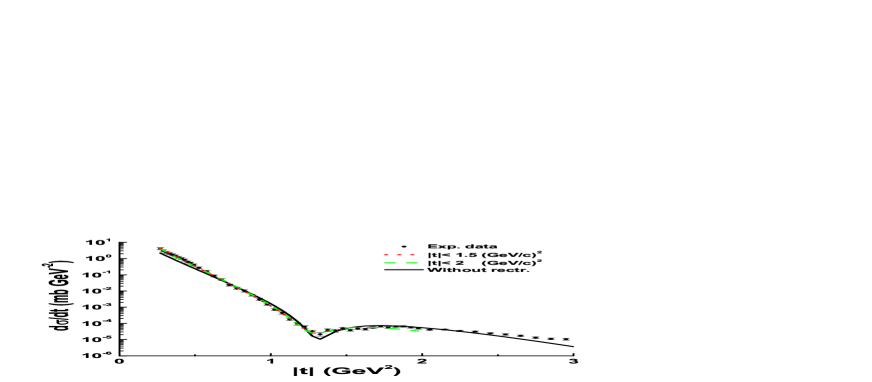
Figure 1: Differential cross section of the elastic $pp$- scattering at $\sqrt{s}=62.3$ GeV. The points are the experimental data [10]. Lines are the fitting results.

A good results of the fitting were obtained for $\bar{p}p$-interactions [13]. More complicated situation took place with the fitting of the $pp$-data. In order to reduce the number of the free parameters, we have fixed $\rho$ using the following parameterizations of the corresponding experimental data from the PDG data-base [14]:

$$\rho_{pp}=0.135-\frac{3}{\sqrt{s}}+\frac{4}{s}+\frac{80}{s^{3}}.$$ (12)

$$\rho_{\bar{p}p}=0.135-\frac{2.26}{\sqrt{s}}.$$ (13)

We assume that this allows us to attract indirectly an additional experimental information because $\rho$ values were measured in the independent experiments – in the Coulomb-nuclear interference region at very small $q$. In principle, $\rho$ can be obtained at the fitting using very exact measurements in the dip region. Such data were presented by the EDDA collaboration [15] for projectile proton momenta, $P_{lab}$, from 1.1 GeV/c up to 3.3 GeV/c. A clear change of the slope of the experimental cross sections was observed at $P_{lab}>$ 2 GeV/c and $\theta_{cms}>60^{o}$. Our obtained $\rho$ values for the data at $P_{lab}>$ 2 GeV/c are in a reasonable agreement with other experimental data [14]. Below 2 GeV/c the 4-parameter fit was unstable due to the parameter’s correlations. Thus we estimate the lower energy boundary of the application region of the present approach as 2 GeV/c for $pp$-interactions. For $\bar{p}p$-interactions the boundary can be smaller.

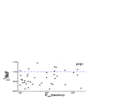
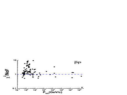
Figure 2: Quality of the fitting of $\bar{p}p$ and $pp$ experimental data.

With all the above given restrictions we have extra-ordinary good fit. $\chi^{2}/NoF=1156/1489\simeq 0.78$ for $pp$-interactions at $P_{lab}\geq 9.9$ GeV/c, and $\chi^{2}/NoF=856/675\simeq 1.27$ for $\bar{p}p$-ones at $P_{lab}\geq 8$ GeV/c. Thus, it seems to us, that we can say about the unified systematic of all high energy (anti)baryon-baryon elastic scattering data.

A quality of the fit is shown in Fig. 2. As seen, most of the $pp$-interactions data are described quite well. The situation is more complicated for the $\bar{p}p$-data especially at low energies. At high energies, the quality of the fitting of $\bar{p}p$-interaction data becomes better.

Some fitting results in a comparison with experimental data are presented in Fig. 3, 4. We show there the experimental data at all measured values of $|t|$ and our results extended outside the fitting region ($|t|<$ 1.75 (GeV/c)²) in order to demonstrate a necessary to include a description of the large angle scattering. As seen, we reproduce the cross sections for $\bar{p}p$-interactions in the fitted region of $|t|$. The dip position is reproduced also.

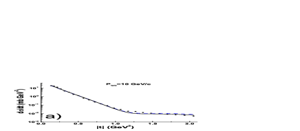
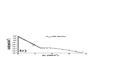
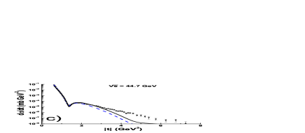
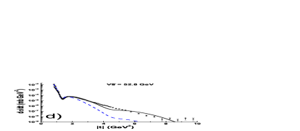
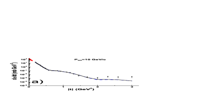
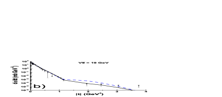
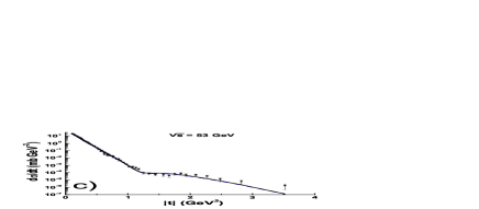
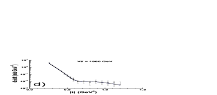
Figure 3: Differential cross sections of elastic proton-proton scatterings. The points are the experimental data (a - [16], b - [17], c - [10], d - [18]). The solid lines are the fitting results without the restriction on $|t|$.

Figure 4: Differential cross sections of elastic antiproton-proton scatterings. The points are the experimental data??? (a - [19], b - [20], c - [21], d - [22]). The solid lines are the fitting results without the restriction on $|t|$.

One can see that the diffraction minimum in $pp$-interactions connected with the first zero of $J_{1}(x)$ shifts to low values of $|t|$ with energy growth. This signals that $R$ is an increasing function of $s$. The filling of the dip is caused by a variation of $\rho$. At $P_{lab}>$ 1.5 GeV/c and $P_{lab}<$ 200 GeV/c $\rho$ is negative. At $P_{lab}\sim$ 200 GeV/c $\rho$ is closed to zero. At larger energy it is positive. So, the filling of the dip depend on energy.

As known, the slope parameter, $B=d\ ln(d\sigma/dt)/dt|_{t\rightarrow 0}$, is increasing function. It is mainly connected with $\pi dq/sinh(\pi dq)$, and with the parameter $d$. So, the parameter $d$ must be increasing function also. The same regularities can be seen for $\bar{p}p$-interactions.

The fitting results for $R$ and $d$ are presented in Fig. 5. They show that $R$ for $\bar{p}p$-interactions decreases with the energy growth starting from low energy, reaches a minimum at $\sqrt{s}\sim 30$ GeV, and continues the growth at higher energies. $R$ for $pp$-interactions in the studied energy range is practically constant.

The energy dependence of $d$ is more complicated. For $pp$-interactions in the considered energy range it is the increasing functions. $d$ for $\bar{p}p$-scattering has an interesting irregularity at very low energies. At high energies it reaches a constant value.

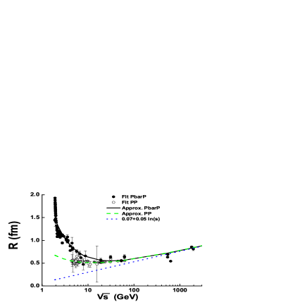
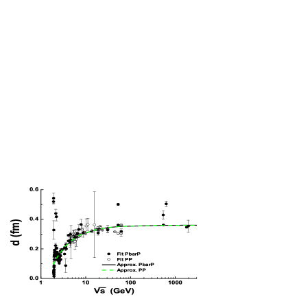
Figure 5: The fitting results for the parameters $R$ and $d$. The black points present the results for $\bar{p}p$-interactions, the open points – for $pp$-interactions.

For future applications we approximate the dependencies as:

$$R_{pp}=0.07+0.05\ln{s}+\frac{0.6}{s^{1/4}}+\frac{0.2}{s^{1/2}},\ \ \ (fm),$$ (14)

$$R_{\bar{p}p}=0.07+0.05\ln{s}+\frac{0.4}{s^{1/4}}+\frac{2}{s^{1/2}},\ \ \ (fm),$$ (15)

$$d_{pp}=d_{\bar{p}p}=0.36-\frac{0.5}{\sqrt{s}}.\ \ \ (fm).$$ (16)

The dependencies are shown in Fig. 5 by the solid and dashed lines. The asymptotical part, $0.07+0.05\ln{s}$, is presented by the dotted line.

The fitting results for the parameters $A$ and $a_{1}$ are shown in Fig. 6. As seen, the parameter $A$ fluctuates within $\pm 30$ % at low energies. It is close to unity at high energies, and there is a defined energy dependence of the parameter. Thus, we believe that the parameter does not reflect only uncertainty of the experimental data normalization, but it contains some information on physics of the processes.

If the parameter $A$ is below unity, it points out on a possible influence of the inelastic shadowing on the elastic scattering due to the processes of excitations and deexcitations of low mass difractive states during the scattering. A value of the parameter above the unity can be interpreted as a presence of additional processes like $\pi$-meson exchange, annihilation and so on which are not taken into account directly. The value above unity can violate the unitarity requirement according to which $|\gamma(b)|$ must be below unity. If $A\leq 1+e^{-R/d}$ there is no problem with the unitariry, but it will mean that the amplitude reaches the black disk limit in the central interactions. If $A>1+e^{-R/d}$ the simplest solution can be an application of any unitarisation scheme. We are going to study the subject in the future.

We show in Fig. 6a the function $1+e^{-R/d}$ for $pp$-interactions by the dashed line. It seems to us that taking into account the fluctuation of the fitting results for the $pp$-interactions at high energies we can assume that the black disk limit is reached in the $pp$-collisions in the central region.

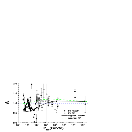
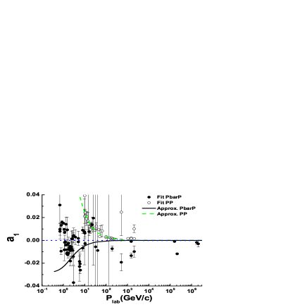
Figure 6: The fitting results for the parameters $A$ and $a_{1}$. The black points present the results for $\bar{p}p$-interactions, the open points – for $pp$-interactions.

As seen in Fig. 6, energy dependence of the parameter $a_{1}$ for $pp$-interaction is rather regular. We cannot say this for $\bar{p}p$-interactions.

For future applications we approximate the dependencies of the parameters $A$ and $a_{1}$ as:

$$A_{pp}=1+e^{-R/d},\ \ \ A_{\bar{p}p}=1+e^{-R/d}-0.6/s^{0.25},$$ (17)

$$a_{1,\ pp}=0.5/s,\ \ \ a_{1,\ \bar{p}p}=-0.1/s.$$ (18)

Using the expressions 12 – 18 we obtain a good description of the $\bar{p}p$- and $pp$-interaction data (see Appendixes). Especially, we have for $pp$-data $\chi^{2}/NoF=4866/1489\simeq 3.26$ at $P_{lab}\geq 9.9$ GeV/c, and for $\bar{p}p$-data – $\chi^{2}/NoF=3620/675\simeq 5.36$ at $P_{lab}\geq 8$ GeV/c having only one fitting parameter – $A$.

2 Description of the Totem data

The expressions 12, 14, 16 predict for the LHC energies the following values of the parameters:

$\sqrt{s}$(GeV)	$R$ (fm)	$d$ (fm)	$\rho$	$\sigma_{tot}$ (mb)	$\sigma_{el}$ (mb)
900	0.770	0.359	0.1316	71.5	16.9
7000	0.963	0.360	0.1346	90.9	22.7
10000	0.997	0.360	0.1347	94.8	24.0
14000	1.030	0.360	0.1348	98.8	25.3

Table 1: Parameters and estimated value for LHC

Using them we calculate total and elastic cross sections, $\sigma_{tot}$ and $\sigma_{el}$.

$$\sigma_{tot}=2\pi\ A\ (R^{2}+\pi^{2}d^{2}/3),$$ (19)

$$\sigma_{el}\simeq\pi\ A^{2}\ (R^{2}-19Rd/10+2\pi^{2}d^{2}/7).$$ (20)

The Totem collaboration [23] published the total and elastic cross sections which are $\sigma_{tot}=98.3\pm 0.2^{stat}\pm 2.8^{sys}$ (mb) and $\sigma_{el}=24.8\pm 0.2^{stat}\pm 1.2^{sys}$ (mb). They are above our predictions. To understand the difference, we calculate differential elastic scattering cross section according to our approach, and the cross section using the simple gaussian parameterization and the value of the slope parameter given by the Collaboration, $B=20.1\pm 0.2^{stat}\pm 0.3^{sys}$ (GeV^-2). They are presented in Fig. 7 by the solid and dashed lines, respectively.

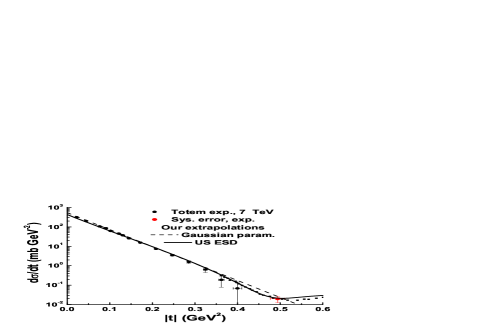
Figure 7: Differential cross section of $pp$ elastic scattering at 7 TeV. The points are the experimental data [24, 23]. The lines are our calculation.

As seen, first of all, the Collaboration fitted the differential cross section at $|t|<$ 0.35 (GeV${}^{-2})$ to obtain the slope and the cross sections (dashed line). Our prediction (solid line) catches the points at $|t|>$ 0.15 (GeV^-2, especially, in the region of the minimum. At $|t|$ below 0.15 (GeV${}^{-2})$ the prediction deviates regularly from the corresponding data. The data are above our curve. Maybe additional expansion terms are needed to be included in Eq. 11. The can give corrections at small $|t|$.

Our description of the data [24, 23] in the whole measured values of $t$ is presented in Fig. 8.

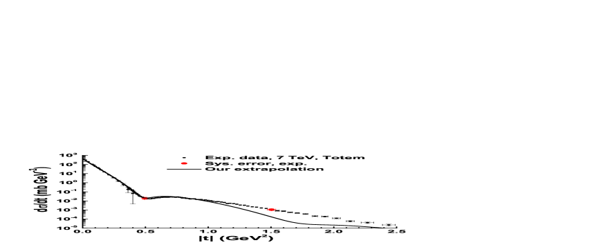
Figure 8: Differential cross section of $pp$ elastic scattering at 7 TeV. The points are the experimental data [24, 23]. The line is our calculation.

One can see that the forward scattering data are reproduced quite well. The dip is filled rather well. Its position is right. At the same time, the calculations deviate from the data starting from lower values of $|t|$ than it was at other energies. The high of the second diffractional maximum is mainly determined by the parameter $d$. The slope of the forward part of the spectra is connected with the parameter also. At chosen value of the parameter we overestimate a little bit the high of the maximum. We can describe better the forward part of the date varying $d$ in its accuracy limits making worse the description of the dip region, and vice-versa. We expect that an exactness of the parameter determination will be improved when the Totem collaboration will publish final data.

We have to note that an accuracy of the parameters entering in Eqs. 14 – 16, 18 is equal to $\pm 5$ %. We expect the same accuracy for the calculated differential cross section. The accuracy can be improved when new Totem data at other energies will be appeared.

In order to understand a quality of the calculations, let us compare our calculations with predictions of other models [25] presented by the Totem collaboration in the paper [24]. For this, we show the model predictions in the dip region and in the region of large $|t|$ in Fig. 9. Because we could not be able to take experimental errors in [24], we plotted the points without errors. Though, the systematic errors are rather large for a correct discrimination of the model, one can see that only our approach gives results that are quite closed to the data at small angles and in the dip region. The high of the second maximum is reproduced also in the approach. But instead of other models we predict too fast decreasing of the cross section above the diffraction maximum. The other models predict much slower decreasing of the cross sections. Here we have to note, that the models were tuned using much less set of experimental data. Additional to this, they included, directly or indirectly, the high momentum transfer scattering.

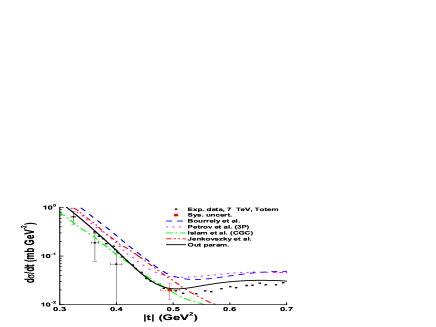
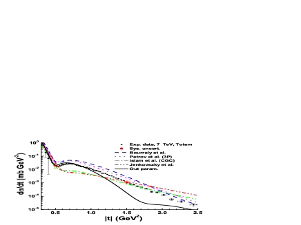
Figure 9: Comparison of model predictions presented in [24] with the Totem experimental data. The solid (black) lines show our calculations.

3 Description of the high momentum part of the data

The nature of processes with high momentum transfer are debated until now. It is commonly accepted that they can be described in QCD. There are a lot of publications on the subject. Instead of analyzing all of them in order to select a reliable one we turn to experimental data. In Fig. 10 we present some experimental data on elastic scattering at large $|t|$.

As seen, at $|t|>$ 2 (GeV/c)² all the cross sections have the same shape at $\sqrt{s}>$ 10 GeV. At the projectile momentum below 200 GeV/c they have strong energy dependence. To reproduce the high energy behavior of the cross sections we add to the imaginary part of the amplitude (11) a ”hard” scattering amplitude:

$$Imf_{hard}(q)=-0.05\ [1+tanh(Rq-5.5)]\frac{1}{(1+|t|/0.71)^{4}}.$$ (21)

The sign ”-” is needed to increase the cross sections in the second maximum where $J_{1}(Rq)$ is negative. The hyperbolic tangent imitates a smooth transition from soft to hard scatterings. According to Fig. 10 the border of the hard processes slowly moves to small momentum transfer with an energy growth. It can be if the border is connected with the radius of the soft interactions. Thus, we assume that the tangent argument is $Rq$. The value ”5.5” gives the exact position of the border. The last factor in Eq. 21 is the proton form-factor in a tuned power. All values in (21) are sampled only in order to reproduce the cross section behavior qualitative at $\sqrt{s}>$ 10 GeV. With all of these we have a description of the Totem data presented in Fig. 11.

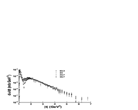
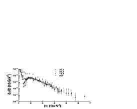
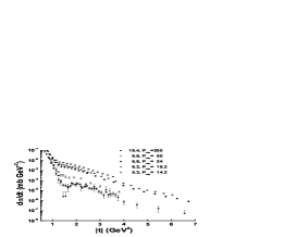
Figure 10: $pp$ elastic scattering data at large momentum transfer. Points are experimental data [10],[21],[18],[26],[17],[16],[27].

Of course, our parameterization of the high momentum part is not perfect one. But at least, it describes the previous experimental data, and we cannot simple disregard it. The behavior of the predictions in Fig. 11 is explained by the variation of $R$. As energy increases, $R$ is increased also, and the yield of the soft part in the high $|t|$ region decreases, the dip is shifted to the lower $|t|$, and the second maximum increases. If we are right, the future measurement of the Totem collaboration can show this. The measurement will give us more information about interplay of the soft and hard interactions.

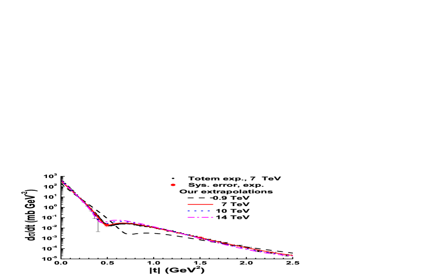
Figure 11: Description of the Totem data and our predictions for other LHC energies.

4 Concluding remarks

4.1 Total and elastic cross sections

According to Exps. (3) and (9) the total cross section is given by the expression:

$$\sigma_{tot}\simeq 2\pi\ A(R^{2}+\pi^{2}d^{2}/3).$$ (22)

For the elastic cross section we have the following expression an exactness of which is about few percent.

$$\sigma_{el}\simeq\pi\ A^{2}(R^{2}-19Rd/20+\pi^{2}d^{2}/7).$$ (23)

They together with Exps. (14) – (17) provide one with a good parameterization of the cross sections.

4.2 Eikonal representation

The profile-function (10) can be represented as an eikonal one:

$$\gamma(b)=1-\left[1-\frac{A}{1+e^{(b-R)/d}}\right]=1-e^{-\ln[(e^{R/d}+e^{b/d})/(e^{b/d}-1)]}.$$ (24)

Here we use the assumption that $A=1+e^{-R/d}$.

It can be used in the Quark-Gluon String Model [8] for a calculations of string multiplicity distributions.

$$P_{n}=\frac{1}{C}\int b\frac{\{2\ln[(e^{R/d}+e^{b/d})/(e^{b/d}-1)]\}^{n}}{n!}\ \ e^{-2\ln[(e^{R/d}+e^{b/d})/(e^{b/d}-1)]}\ db.$$ (25)

4.3 Application of USESD in calculations of hadron-nucleus and nucleus-nucleus properties.

An amplitude for an elastic scattering of an nucleus containing $B$ baryons on a target nucleus with mass number $A$ is given as [28]:

$$F_{BA}(\vec{q})=\frac{i}{2\pi}\ \int d^{2}b\ e^{i\vec{q}\vec{b}}\ \left\{1-\prod^{B}_{i=1}\prod^{A}_{j=1}\left[1-\gamma(\vec{b}+\vec{\tau}_{i}-\vec{s}_{j})\right]\right\}|\Psi_{B}|^{2}|\Psi_{A}|^{2}\ \left(\prod^{B}_{i=1}d^{3}\ t_{i}\right)\ \left(\prod^{A}_{j=1}d^{3}\ r_{j}\right)$$ (26)

$$=i\ \int^{\infty}_{0}bP_{BA}(b)\ J_{0}(qb)db,$$

where $\gamma$ is an amplitude of an elastic nucleon-nucleon scattering in the impact parameter representation, averaged over the spin and isospin degrees of freedom,

$$\gamma(\vec{b})=\frac{1}{2\pi i}\int d^{2}q\ e^{i\vec{q}\vec{b}}f(\vec{q}).$$

$\Psi_{A}\ (\Psi_{B})$ is the wave function of the target (projectile) nucleus in the ground state. Taking the origin of the coordinate system to coincide with the center of the nucleus, the nucleon coordinates ($\{\vec{r}_{A}\}$, $\{\vec{t}_{B}\}$) are decomposed into longitudinal ({$z_{i}$}) and transverse ($\{\vec{s}_{j}\}$, $\{\vec{\tau}_{i}\}$) components. The $z$-axis is directed along the projectile momentum. $\vec{b}$ is the impact parameter vector orthogonal to the momentum. $P_{BA}(b)$ is the profile function and $J_{0}$ is the Bessel function of zero order.

Quite often $\gamma$ is parameterized as:

$$\gamma(\vec{b})=\frac{\sigma^{tot}_{NN}\ (1-i\rho)}{4\pi\ \beta}\ e^{-\vec{b}^{2}/2\beta},$$ (27)

where $\sigma^{tot}_{NN}$ is the total cross section of the nucleon-nucleon interactions, $\rho$ is the ratio of the real to imaginary parts of the $NN$ elastic scattering amplitude at zero momentum transfer, and $\beta$ is a slope parameter of the $NN$ differential elastic scattering cross section. Then

$$f(\vec{q})=\frac{i}{4\pi}\sigma^{tot}_{NN}\ (1-i\rho)\ e^{-\beta\vec{q}^{2}/2},\ \ \$$ (28)

$\beta$ can be found as:

$$\beta=(\sigma^{tot}_{NN})^{2}(1+|\rho|^{2})/(16\ \pi\ \sigma^{el}_{NN}\ 0.3897).$$

Here, $\sigma^{el}_{NN}$ is the $NN$ elastic cross section and $0.3897$ is a coefficient required in order to express $\beta$ in units of $(GeV/c)^{-2}$, if the cross sections are given in millibarns.

The squared modulus of the wave function is usually written as:

$$|\Psi_{A}|^{2}=\delta(\sum_{i=1}^{A}\vec{r}_{i}/A)\ \prod_{i=1}^{A}\rho_{A}(\vec{r}_{i}).$$ (29)

$\rho_{A}$ coincides with the one-particle density of the nucleus if one neglects the center-of-mass correlation connected with the $\delta$ function.

We have used Exp. (27) at the calculation of the differential elastic scattering cross section at $\sqrt{s}=7$ TeV, results of which are shown in Fig. 7 as the dashed line (Gaussian param.). It is obvious, that it can describe the cross sections only at small value of $|t|$. It would be better to use Exp. (10) for more exact calculations as nucleon-nucleon interaction properties, as well as baryon-nucleus and nucleus-nucleus ones.

The task is very actual for calculations of wounded nucleon multiplicities in nucleus-nucleus interactions at high energies.

4.4 Comparison of USESD with other approaches

Many years ago T.-Y. Cheng, S.-Y. Chu and A.W. Hendry [29] successfully used 2-dimensional Fermi-function to describe $pp$ elastic scattering at all angles from 3 to 24 GeV/c. They analyzed polarized proton scattering by proton. Most probably is that they used numerical integration. We have used analytical expressions, and we have considered only unpolarized proton scattering.

In 2000 M. Kawasaki, T. Maehara and M. Yonezawa analyzing the general structure of the elastic scattering amplitude in the impact parameter representation proposed the following expression for the amplitude in the momentum representation [30]:

$$Im\ f(q)\propto R^{2}\left[\frac{J_{1}(Rq)}{Rq}\Phi_{0}(R,q)+\frac{J_{0}(Rq)}{\mu q}\Phi_{1}(R,q)\right],$$ (30)

where $\mu$ is a parameter. They proposed also a concrete form of the dumping functions:

$$\Phi_{0}(R,q)=Re\ \Gamma\left(1+i\frac{q}{\mu}\right),\ \ \ \Phi_{1}(R,q)=-Im\ \Gamma\left(1+i\frac{q}{\mu}\right).$$

They were trying to fit the high energy $\bar{p}p$- and $pp$-data [31, 32] but results were not impressive. Especially, in the paper [32] the authors fitted the differential cross sections of $pp$ elastic scattering at $\sqrt{s}\geq 23.5$ GeV and the $\bar{p}p$-data at $\sqrt{s}\geq 546$ GeV. Only small momentum transfer region, $0.02\leq|t|\leq 0.2$ (GeV/c)², was included in the fit.

In our paper we have considered much larger energy region and a larger region of the momentum transfer. We assume our results as promising ones. Thus a choice of the dumping functions is very important for a correct reproduction of experimental data.

P. Gauron, B. Nicolescu and E. Leader proposed in the paper [33] the following expressions for asymptotic parts of (anti) proton-proton elastic scattering amplitude:

$$\frac{1}{is}F_{+}(s,t)=F_{1}\ ln^{2}(\bar{s})\frac{2J_{1}(R_{+}\bar{\tau})}{R_{+}\bar{\tau}}\ e^{b^{+}_{1}t}+F_{2}\ ln(\bar{s})J_{0}(R_{+}\bar{\tau})\ e^{b^{+}_{2}t}+$$ (31)

$$F_{3}\left[J_{0}(R_{+}\bar{\tau})-R_{+}\bar{\tau}\ J_{1}(R_{+}\bar{\tau})\right]\ \ e^{b^{+}_{3}t},$$

$$\frac{1}{s}F_{-}(s,t)=O_{1}\ ln^{2}(\bar{s})\frac{sin(R_{-}\bar{\tau})}{R_{+}\bar{\tau}}\ e^{b^{-}_{1}t}+O_{2}\ ln(\bar{s})cos(R_{-}\bar{\tau})\ e^{b^{-}_{2}t}+O_{3}\ e^{b^{-}_{3}t},$$ (32)

where $\bar{s}=\frac{s}{s_{0}}e^{-i\pi/2}$; $\bar{\tau}=\left(-\frac{t}{t_{0}}\right)^{1/2}ln(\bar{s})$; $s_{0}=t_{0}=1$ GeV²; $F_{i}$, $O_{i}$, $b_{i}$, $R_{+}$ and $R_{-}$ are constants.

$$F_{pp}=F_{+}\ +\ F_{-},\ \ \ F_{\bar{p}p}=F_{+}\ -\ F_{-}.$$

The appearance of the exponents in the expressions is connected with the simplest assumption about the functional form of the residue functions. If one replaces the exponents by $\pi d\sqrt{-t}/sinh(\pi d\sqrt{-t})$ then the leading term of $F_{+}$ will be coincided with the first term of our expression (11). Thus our approach corresponds to the approach of the authors at defined assumptions on the residue functions. But instead of the authors we did not assume any energy dependence of our parameter $R$. We obtained it at the fitting of the experimental data.

If we suppose that $R=R_{0}+\Delta R$ where $\Delta R\propto s^{-\alpha_{R}}$, and expand the first term of Eq. 11 we will have yields of ”non-dominant Regge pole contributions” into the scattering amplitude.

Very often in a Regge-like analysis the elastic scattering amplitude of a process $1+2\rightarrow 1+2$ is represented as:

$$\gamma(b)=\frac{1}{C_{1}C_{2}}(1-e^{-\omega(b)}),$$ (33)

where

$$\omega(b)=\frac{\eta C_{1}C_{2}g_{1}(0)g_{2}(0)}{R_{1}^{2}+R_{2}^{2}+\alpha^{\prime}\xi^{\prime}}\ e^{\Delta\xi}\ e^{-b^{2}/4(R_{1}^{2}+R_{2}^{2}+\alpha^{\prime}\xi^{\prime})},$$ (34)

$\eta=1+icotan(\pi\alpha_{P}(0)/2)$ is a signature factor; $C_{1}$ ($C_{2}$) – shower enhancement coefficient in the interaction vertex of the first (second) particle with a reggeon/pomeron; $\alpha_{P}(0)=1+\Delta$ is an intercept of the reggeon/pomeron; $\xi=ln\ s_{12}$ is a logarithm of CMS energy squared; $\xi^{\prime}=\xi-i\pi/2$. It is assumed that Regge trajectories are linear, $\alpha(t)=1+\Delta+\xi^{\prime}t$. Non-linear trajectories were considered in [35]. It is assumed also that the residue functions have the gaussian shape – $g_{i}(t)=g_{i}(0)exp(R^{2}_{i}\ t)$, for simplicity.

It is complicated to find a correspondence between the eikonal 34 and our eikonal 24. Though, the structure of the eikonal 34 is rather simple – it is a product of a function of $b$, and a factor strongly dependented on the energy – $e^{\Delta\xi}$. For our eikonal at large $b$ and $C_{1}=C_{2}=1$, we have:

$$\omega(b)=\ln[(e^{R/d}+e^{b/d})/(e^{b/d}-1)]|_{b\rightarrow\infty}\simeq e^{-b/d}[e^{R/d}+1].$$

Thus the energy dependence of the eikonal is determined by $e^{R/d}\simeq s^{0.1/d}\simeq s^{0.28}$. Here we take into account that $R\propto 0.1\ln s$, and $d\propto 0.36$. So, an effective intercept in our model is 1.28. It is in a correspondence with results of papers [35, 36].

Summing up, we can say that our model is in the main stream of phenomenological analysis of the elastic scattering data. The model assumes the defined choice of the dumping functions, or the residue functions. A correct form of the functions is very important for high energy phenomenology.

The authors are thankful to the Geant4 hadronic working group for interest in the work.

Appendix A: Comparison of experimental data on $pp$-interactions with USESD parameterization

Figure 12: The points are the experimental data by R.M. Edelstein et al., Phys. Rev. D5 (1972) 1073.

Figure 13: The points are the experimental data by J.V. Allaby et al., Nucl. Phys. B52 (1973) 316.

Figure 14: The points are the experimental data by G.W. Brandenburg et al., Phys. Lett. 58B (1975) 367.

Figure 15: The points are the experimental data by K.J. Foley et al., Phys. Rev. Lett. 11 (1963) 425.

Figure 16: The points are the experimental data by K.J. Foley et al., Phys. Rev. Lett. 15 (1965) 45.

Figure 17: The points are the experimental data by J.V. Allaby et al., Nucl. Phys. B52 (1973) 316.

Figure 18: The points are the experimental data by D. Harting, Nuovo Cimento 38 (1965) 60.

Figure 19: The points are the experimental data by K.J. Foley et al., Phys. Rev. Lett. 11 (1963) 425.

Figure 20: The points are the experimental data by J.V. Allaby et al., Nucl. Phys. B52 (1973) 316.

Figure 21: The points are the experimental data by K.J. Foley et al., Phys. Rev. Lett. 11 (1963) 425.

Figure 22: The points are the experimental data by R.M. Edelstein et al., Phys. Rev. D5 (1972) 1073.

Figure 23: The points are the experimental data by .K.J. Foley et al., Phys. Rev. Lett. 11 (1963) 425

Figure 24: The points are the experimental data by D. Harting, Nuovo Cimento 38 (1965) 60.

Figure 25: The points are the experimental data by J.V. Allaby et al., Phys. Lett. B28 (1968) 67.

Figure 26: The points are the experimental data by .K.J. Foley et al., Phys. Rev. Lett. 11 (1963) 425

Figure 27: The points are the experimental data by R.M. Edelstein et al., Phys. Rev. D5 (1972) 1073.

Figure 28: The points are the experimental data by J.V. Allaby et al., Phys. Lett. B28 (1968) 67.

Figure 29: The points are the experimental data by J.V. Allaby et al., Nucl. Phys. B52 (1973) 316.

Figure 30: The points are the experimental data by R.M. Edelstein et al., Phys. Rev. D5 (1972) 1073.

Figure 31: The points are the experimental data by R. Rusack et al., Phys. Rev. Lett. 41 (1978) 1632.

Figure 32: The points are the experimental data by C. Bruneton et al., Nucl. Phys. B124 (1977) 391.

Figure 33: The points are the experimental data by Z. Asad et al., Nucl. Phys. B255 (1984) 273; C.W. Akerlof et al., Phys. Rev. D14 (1976) 2864; D.S. Ayres et al., Phys. Rev. D15 (1977) 3105.

Figure 34: The points are the experimental data by R. Rusack et al., Phys. Rev. Lett. 41 (1978) 1632.

Figure 35: The points are the experimental data by R. Rusack et al., Phys. Rev. Lett. 41 (1978) 1632.

Figure 36: The points are the experimental data by D.S. Ayres et al., Phys. Rev. D15 (1977) 3105.

Figure 37: The points are the experimental data by C.W. Akerlof et al., Phys. Rev. D14 (1976) 2864; R. Rubinstein et al., Phys. Rev.D30 (1984) 1413.

Figure 38: The points are the experimental data by D.S. Ayres et al., Phys. Rev. D15 (1977) 3105; R. Rusack et al., Phys. Rev. Lett. 41 (1978) 1632.

Figure 39: The points are the experimental data by R. Rusack et al., Phys. Rev. Lett. 41 (1978) 1632.

Figure 40: The points are the experimental data by D.S. Ayres et al., Phys. Rev. D15 (1977) 3105.

Figure 41: The points are the experimental data by D. Brick et al., Phys. Rev. D25 (1982) 2794.

Figure 42: The points are the experimental data by R. Rusack et al., Phys. Rev. Lett. 41 (1978) 1632.

Figure 43: The points are the experimental data by R. Rusack et al., Phys. Rev. Lett. 41 (1978) 1632.

Figure 44: The points are the experimental data by D.S. Ayres et al., Phys. Rev. D15 (1977) 3105.

Figure 45: The points are the experimental data by R. Rusack et al., Phys. Rev. Lett. 41 (1978) 1632.

Figure 46: The points are the experimental data by C.W. Akerlof et al., Phys. Rev. D14 (1976) 2864; R. Rubinstein et al., Phys. Rev.D30 (1984) 1413.

Figure 47: The points are the experimental data by A. Schiz et al., Phys. Rev. D24 (1981) 26; G. Fidecaro et al., Nucl. Phys. B173 (1980) 513.

Figure 48: The points are the experimental data by R. Rusack et al., Phys. Rev. Lett. 41 (1978) 1632.

Figure 49: The points are the experimental data by R. Rusack et al., Phys. Rev. Lett. 41 (1978) 1632.

Figure 50: The points are the experimental data by R. Rusack et al., Phys. Rev. Lett. 41 (1978) 1632.

Figure 51: The points are the experimental data by M.G. Albrow et al., Nucl. Phys. B108 (1976) 1.

Figure 52: The points are the experimental data by U. Amaldi and K.R. Schubert, Nucl. Phys. B166 (1980) 301.

Figure 53: The points are the experimental data by M.G. Albrow et al., Nucl. Phys. B108 (1976) 1.

Figure 54: The points are the experimental data by U. Amaldi and K.R. Schubert, Nucl. Phys. B166 (1980) 301.

Figure 55: The points are the experimental data by A. Breakstone et al. Nucl. Phys. B248 (1984) 253.

Figure 56: The points are the experimental data by U. Amaldi and K.R. Schubert, Nucl. Phys. B166 (1980) 301.

Figure 57: The points are the experimental data by E. Nagy et al., Nucl. Phys. B150 (1979) 221.

Figure 58: The points are the experimental data by A. Breakstone et al. Nucl. Phys. B248 (1984) 253; Phys. Rev. Lett. 54 (1985) 2180.

Figure 59: The points are the experimental data by S. Erhan et al., Phys. Lett. B152 (1985) 131; J.C.M. Armitage et al., Nucl. Phys. B132 (1978) 365.

Figure 60: The points are the experimental data by A. Breakstone et al. Nucl. Phys. B248 (1984) 253.

Figure 61: The points are the experimental data by N. Amos et al., Nucl. Phys. B262 (1985) 689.

Figure 62: The points are the experimental data by U. Amaldi and K.R. Schubert, Nucl. Phys. B166 (1980) 301.

Figure 63: The points are the experimental data by U. Amaldi and K.R. Schubert, Nucl. Phys. B166 (1980) 301.

Appendix B: Comparison of experimental data on $\bar{p}p$-interactions with USESD parameterization

Figure 64: The points are the experimental data by J.S. Russ et al., Phys. Rev. D15 (1977) 3139.

Figure 65: The points are the experimental data by D.P. Owen et al., Phys. Rev. 181 (1969) 1794.

Figure 66: The points are the experimental data by A. Berglund et al., Nucl. Phys. B176 1980) 346.

Figure 67: The points are the experimental data by G. Brandenburg et al., Phys. Lett. 58B (1975) 367.

Figure 68: The points are the experimental data by K.J. D. Birnbaum et al., Phys. Rev. Lett. 23 (1969) 663.

Figure 69: The points are the experimental data by B. Batyunya et al. Yad. Fiz. 44 (1986) 1489.

Figure 70: The points are the experimental data by Yu.M. Antipov et al., Nucl. Phys. B57 (1973) 333.

Figure 71: The points are the experimental data by M.Y. Bogolyubsky et al., Yad. Fiz. 41 (1985) 1210.

Figure 72: The points are the experimental data by Yu.M. Antipov et al., Nucl. Phys. B57 (1973) 333.

Figure 73: The points are the experimental data by R.L. Cool et al., Phys. Rev. D24 (1981) 2821.

Figure 74: The points are the experimental data by A. Breakstone et al., Nucl. Phys. B248 (1984) 253, Phys. Rev. Lett. 54 (1985) 2180.

Figure 75: The points are the experimental data by A. Breakstone et al., Nucl. Phys. B248 (1984) 253, Phys. Rev. Lett. 54 (1985) 2180.

Figure 76: The points are the experimental data by A. Breakstone et al., Nucl. Phys. B248 (1984) 253, Phys. Rev. Lett. 54 (1985) 2180.

Figure 77: The points are the experimental data by G. Arnison et al., Phys. Lett. B128 (1983) 336.

Figure 78: The points are the experimental data by M. Bozzo et al., Phys. Lett. B155 (1985) 197, Phys. Lett. B147 (1984) 385.

Figure 79: The points are the experimental data by D. Bernard et al., Phys. Lett. B198 (1987) 583, Phys. Lett. B171 (1986) 142.

Figure 80: The points are the experimental data by N. Amos et al., Nucl. Phys. B262 (1985) 689, Phys. Lett. B247 (1990) 127.

Figure 81: The points are the experimental data by the D0 Collaboration – D0 Note 6056-CONF.

Appendix C: Quality of the data fitting
$\chi^{2}$ presented below is obtained with values of the parameters given by Eqs. 12 – 16, 18. $N$ is number of experimental points. $N_{F}$ - the number of points included in the fitting.

Table 2: Fitting results for $pp$-interactions

$P_{lab}$	$\sqrt{s}$	$N$	$N_{F}$	$\chi^{2}/NoF$	A	$R$	$d$	$\rho$	$a_{1}$
(GeV/c)	(GeV)					(fm)	(fm)		(fm2)
9.9	4.523	28	28	0.560	1.180$\pm$ 0.018	0.547	0.249	-0.323	0.0244
10	4.543	24	21	8.66	0.746 $\pm$ 0.016	0.547	0.250	-0.322	0.0242
10.4	4.625	97	97	2.56	1.244 $\pm$ 0.002	0.545	0.252	-0.319	0.0234
10.8	4.705	13	13	2.70	1.177 $\pm$ 0.012	0.544	0.254	-0.315	0.0226
10.9	4.733	9	9	0.72	1.108 $\pm$ 0.014	0.544	0.254	-0.313	0.0223
12	4.939	25	18	8.48	0.845 $\pm$ 0.019	0.540	0.259	-0.303	0.0205
12.4	5.014	22	21	0.72	1.065 $\pm$ 0.012	0.539	0.260	-0.299	0.0199
12.8	5.088	13	13	2.96	1.180 $\pm$ 0.013	0.538	0.262	-0.296	0.0193
14.2	5.34	22	12	4.32	0.818 $\pm$ 0.021	0.535	0.266	-0.283	0.0175
14.8	5.444	12	12	1.98	1.159 $\pm$ 0.014	0.533	0.268	-0.278	0.0169
15.1	5.496	32	25	0.22	1.200 $\pm$ 0.019	0.533	0.269	-0.276	0.0166
16.7	5.762	12	12	1.22	1.154 $\pm$ 0.014	0.530	0.273	-0.263	0.0151
18.4	6.033	20	18	1.32	1.076 $\pm$ 0.016	0.527	0.277	-0.251	0.0137
19.2	6.156	27	19	14.4	0.899 $\pm$ 0.011	0.526	0.279	-0.245	0.0132
19.6	6.217	11	11	1.82	1.132 $\pm$ 0.014	0.526	0.280	-0.243	0.0129
20	6.277	30	28	2.92	1.043 $\pm$ 0.016	0.525	0.280	-0.240	0.0127
21.12	6.442	17	15	12.04	0.946 $\pm$ 0.011	0.524	0.282	-0.233	0.0121
24	6.849	35	20	5.62	1.000 $\pm$ 0.015	0.521	0.287	-0.217	0.0107
29.7	7.591	29	25	1.60	1.060 $\pm$ 0.018	0.517	0.294	-0.190	0.0087
35	8.221	21	19	1.30	1.120 $\pm$ 0.022	0.514	0.299	-0.171	0.0074
44.5	9.243	27	25	7.28	1.093 $\pm$ 0.004	0.511	0.306	-0.143	0.0059
50	9.787	33	27	11.06	1.106 $\pm$ 0.006	0.510	0.309	-0.130	0.0052
55.4	10.29	20	17	1.38	1.047 $\pm$ 0.022	0.510	0.311	-0.119	0.0047
65	11.13	20	17	1.14	1.134 $\pm$ 0.024	0.509	0.315	-0.102	0.0040
70	11.55	17	17	2.26	1.136 $\pm$ 0.006	0.509	0.317	-0.095	0.0037
100	13.78	81	69	1.22	1.147 $\pm$ 0.007	0.509	0.324	-0.062	0.0026
100	13.78	37	34	1.62	1.125 $\pm$ 0.006	0.509	0.324	-0.062	0.0026
130	15.69	11	11	0.34	1.137 $\pm$ 0.030	0.510	0.328	-0.040	0.0020
140	16.28	19	19	3.56	1.124 $\pm$ 0.006	0.510	0.329	-0.034	0.0019
150	16.85	31	26	0.60	1.107 $\pm$ 0.021	0.511	0.330	-0.029	0.0018
170	17.93	29	23	0.60	1.154 $\pm$ 0.024	0.512	0.332	-0.020	0.0016
175	18.19	15	15	2.82	1.139 $\pm$ 0.007	0.512	0.333	-0.018	0.0015
190	18.95	30	24	1.18	1.098 $\pm$ 0.023	0.513	0.334	-0.012	0.0014
200	19.44	90	58	1.44	1.104 $\pm$ 0.007	0.513	0.334	-0.009	0.0013
200	19.44	167	156	2.48	1.080 $\pm$ 0.002	0.513	0.334	-0.009	0.0013
210	19.91	29	23	0.72	1.095 $\pm$ 0.025	0.514	0.335	-0.006	0.0013
230	20.84	19	16	2.34	1.064 $\pm$ 0.030	0.515	0.336	0.000	0.0012
250	21.72	17	14	0.68	1.167 $\pm$ 0.033	0.516	0.337	0.005	0.0011
292	23.47	19	19	0.26	1.186 $\pm$ 0.024	0.518	0.339	0.014	0.0009
293.5	23.53	133	97	5.56	1.067 $\pm$ 0.003	0.518	0.339	0.015	0.0009
497	30.6	15	15	0.56	1.249 $\pm$ 0.027	0.527	0.344	0.041	0.0005
501.3	30.73	124	88	2.32	1.135 $\pm$ 0.003	0.527	0.344	0.042	0.0005
512	31.05	24	24	0.48	1.100 $\pm$ 0.015	0.528	0.344	0.043	0.0005
1064	44.74	65	26	3.80	1.032 $\pm$ 0.008	0.544	0.349	0.070	0.0002
1486	52.87	63	19	3.48	0.982 $\pm$ 0.014	0.553	0.351	0.080	0.0002
1497	53.07	55	41	1.20	1.027 $\pm$ 0.013	0.553	0.351	0.080	0.0002
1497	53.07	27	24	3.82	1.143 $\pm$ 0.009	0.553	0.351	0.080	0.0002
2048	62.06	23	23	0.58	1.094 $\pm$ 0.013	0.562	0.352	0.087	0.0001
2077	62.5	74	37	4.20	1.000 $\pm$ 0.014	0.563	0.352	0.088	0.0001
2081	62.56	49	49	13.6	0.996 $\pm$ 0.001	0.563	0.352	0.088	0.0001

Table 3: Fitting results for $\bar{p}p$-interactions

$P_{lab}$	$\sqrt{s}$	$N$	$N_{F}$	$\chi^{2}/NoF$	A	$R$	$d$	$\rho$	$a_{1}$
(GeV/c)	(GeV)					(fm)	(fm)		(fm2)
8.00	4.111	41	41	4.42	0.833 $\pm$ 0.0008	0.895	0.238	-0.320	-0.005916
9.71	4.483	10	5	1.90	0.618 $\pm$ 0.0427	0.855	0.249	-0.320	-0.004975
10.1	4.564	35	31	5.04	0.880 $\pm$ 0.0042	0.847	0.250	-0.320	-0.004801
10.4	4.625	61	61	3.68	0.881 $\pm$ 0.0008	0.842	0.252	-0.320	-0.004675
16.0	5.647	23	23	2.38	0.834 $\pm$ 0.0023	0.766	0.272	-0.265	-0.003136
22.4	6.626	44	44	1.28	0.910 $\pm$ 0.0047	0.716	0.285	-0.206	-0.002277
25.2	7.012	33	33	2.00	0.885 $\pm$ 0.0040	0.701	0.289	-0.187	-0.002034
32.1	7.882	52	52	4.98	0.893 $\pm$ 0.0035	0.673	0.297	-0.152	-0.001609
40.1	8.785	33	33	1.08	0.888 $\pm$ 0.0068	0.650	0.303	-0.122	-0.001296
191.1	19.1	27	23	2.28	0.974 $\pm$ 0.0182	0.562	0.334	0.016	-2.770E-4
510.2	31.0	22	22	1.44	1.076 $\pm$ 0.0080	0.550	0.344	0.062	-1.041E-4
	53.0	51	44	3.94	1.015 $\pm$ 0.0053	0.560	0.351	0.092	-3.560E-5
	62.3	23	23	1.12	1.068 $\pm$ 0.0063	0.566	0.352	0.099	-2.576E-5
	540	36	36	0.84	1.090 $\pm$ 0.0062	0.720	0.359	0.131	-3.429E-7
	546	121	121	17.24	1.143 $\pm$ 0.0018	0.721	0.359	0.131	-3.354E-7
	630	19	15	7.66	1.124 $\pm$ 0.0147	0.734	0.359	0.131	-2.520E-7
	1800	51	51	1.04	1.085 $\pm$ 0.0028	0.830	0.360	0.134	-3.086E-8
	1960	17	17	0.36	1.095 $\pm$ 0.0323	0.838	0.360	0.134	-2.603E-8

Appendix D: Attempt to fit the COSY data on $pp$-interactions – D. Albers et al.,Phys. Rev. Lett. 78 (1997) 1652.
We represent the elastic scattering amplitude in the energy range, 1 – 3 GeV/c as

$$F_{pp}=f(\theta)+f(\pi-\theta),$$

where $f(\theta)$ is given by Eq. 11. Below the lines are results of a fit with 4 free parameters – $A$, $R$, $d$ and $a_{1}$.

Figure 82: The points are the experimental data.

Figure 83: The points are the experimental data.

Figure 84: The points are the experimental data.

Figure 85: The points are the experimental data.

Figure 86: The points are the experimental data.

Figure 87: The points are the experimental data.

Figure 88: The points are the experimental data.

Figure 89: The points are the experimental data.

Figure 90: The points are the experimental data.

Figure 91: The points are the experimental data.

References

- [1] I.S. Gradstein, I.M. Ruzhik, ”Tables of Integrals, Series and Products”, 1980, New York, Academic.
- [2] A. Grossmann and J. Morlet, SIAM Math. Anal. 15 (1984) 723; ”Wavelet Analysis and Its Applications”, San Diego, Academ. Press Inc., 1992;
- [3] J.S. Blair, Phys. Rev. 95 (1954) 1218; J.A.McIntyre, K.H. Wang, L.C. Becker, Phys. Rev. 117 (1960) 1317; E.V. Inopin, Sov. Phys. JETP 21 (1965) 1090; T.E.O. Ericson, ”Preludes in Theoretical Physics”, Ed. A. De-Shalit, H. Feshbach, L. Van Hove, Amsterdam, 1966, p. 321; A.V. Shebeko, Sov. J. Nucl. Phys. 5 (1967) 543.
- [4] W.E. Frahn and R.H. Venter, Ann. Phys. 24 (1963) 234; W.E. Frahn, Nucl. Phys. A302 (1978) 267, Nucl. Phys. A302 (1978) 281.
- [5] D.W.L. Sprung and J. Martorell, J. Phys. A30 (1997) 6525; A31 (1998) 8973.
- [6] P. Brogueira and J. Dias de Deus, Eur. Phys. J. 37 (2010) 075006).
- [7] M.M. Block and R.N. Cahn, Rev. Mod. Phys. 57 (1985) 563.
- [8] A. Capella and J. Tran Thanh Van, Z. Phys. C10 (1981) 249; A. Capella, U. Sukhatme, C.-I. Tan, J. Tran Thanh Van, Phys. Rep. 236 (1994) 225; A.B. Kaidalov and K.A. Ter-Martirosyan, Phys. Lett. B117 (1982) 247.
- [9] X-.N. Wang and M. Gyulassy, Phys. Rev. D44 (1991) 3501; M. Gyulassy and X-.N. Wang, Comp. Phys. Commun. 83 (1994) 307.
- [10] U. Amaldi and K.R. Schubert, Nucl. Phys. B166 (1980) 301.
- [11] http://www.theo.phys.ulg.ac.be/cudell/data
- [12] J.R. Cudell, A. Lengyel and E. Martynov, Phys. Rev. D73 (2006) 034008.
- [13] A.S. Galoyan and V.V. Uzhinskii, JETP Lett. 97 (2011) 499.
- [14] Particle Data Group, http://pdg.lbl.gov/2009/hadronic-xsections/hadron.html
- [15] D. Albers et al.,Phys. Rev. Lett. 78 (1997) 1652.
- [16] J.V. Allaby et al., Nucl. Phys. B52 (1973) 316.
- [17] Z. Asad et al., Nucl. Phys. B255 (1984) 273; C.W. Akerlof et al., Phys. Rev. D14 (1976) 2864; D.S. Ayres et al., Phys. Rev. D15 (1977) 3105.
- [18] E. Nagy et al., Nucl. Phys. B150 (1979) 221.
- [19] A. Berglund et al., Nucl. Phys. B176 1980) 346.
- [20] R.L. Cool et al., Phys. Rev. D24 (1981) 2821.
- [21] A. Breakstone et al., Nucl. Phys. B248 (1984) 253; Phys. Rev. Lett. 54 (1985) 2180.
- [22] D0 Collaboration, D0 Note 6056-CONF.
- [23] TOTEM Collaboration, G. Antchev et al. Europhys. Lett. 96 (2011) 21002.
- [24] TOTEM Collaboration, G. Antchev et al. Europhys. Lett. 95 (2011) 41001.
- [25] M.M. Block and F. Halzen, Phys. Rev. D83 (2011) 077901; C. Bourrely et al., Eur. Phys. J. C28 (2003) 97; M. Islam et al., Mod. Phys. Lett. A24 (2009) 485; L. Jenkovzky et al., arXiv:1106.3299 [hep-ph]; V. Petrov et al., Eur. Phys. J. C28 (2003) 525.
- [26] R. Rubinstein et al., Phys. Rev.D30 (1984) 1413, Phys. Rev. Lett. 30 (1973) 1010.
- [27] J.V. Allaby et al., Phys. Lett. B28 (1968) 67.
- [28] V.Franco, Phys. Rev. 175 (1968) 1376.
- [29] T.-Y. Cheng, S.-Y. Chu and A.W. Hendry, Phys. Rev. D7 (1973) 86.
- [30] M. Kawasaki, T. Maehara and M. Yonezawa, Phys. Rev. D62 (2000) 074005.
- [31] M. Kawasaki, T. Maehara and M. Yonezawa, Mod. Phys. Lett. A19 (2004) 3001.
- [32] M. Kawasaki, T. Maehara and M. Yonezawa, Phys. Rev. D70 (2004) 114024.
- [33] P. Gauron, B. Nicolescu and E. Leader, Nucl. Phys. B299 (1988) 640.
- [34] A. Sibirtsev et al., Eur. Phys. J. A45 (2010) 357.
- [35] A.A. Godizov, Phys. Lett. B703 (2011) 331.
- [36] V.A. Petrov and A.V. Prokudin, Eur. Phys. J. C23 (2002) 135.