Abstract

Results of monitoring the H₂O and OH masers in W44C, located near the cometary HII region G34.3$+$0.15, are reported. Observations in the water-vapor line at $\lambda=1.35$ cm were carried out on the 22-meter radio telescope of the Pushchino Radio Astronomy Observatory (Russia) from November 1979 to March 2011, and in the hydroxyl lines at $\lambda=18$ cm on the Large Nançay radio telescope (France). Activity maxima and minima of the water maser alternated. The average period of the activity is $\sim 14$ years, consistent with results obtained earlier for a number of other sources associated with regions of active star formation. In periods of enhanced maser activity, two series of strong H₂O maser flares were observed, which were related to two different clusters of maser spots located at the front of a shock at the periphery of the ultracompact region UH II. These series of flares may be associated with cyclic activity of the protostellar object in UH II. In the remaining time intervals, there were mainly short-lived flares of single features. The Stokes parameters for the observations in the hydroxyl lines were determined. Zeeman splitting was observed in the profile of the 1667 MHz OH main line at a velocity of 58.5 km/s, and was used estimate the intensity of the line-of-sight component of the magnetic field (1.2 mG).

1 INTRODUCTION

The source G34.3$+$0.15 is in a region of active star formation, (distance 3.8 kpc) which hosts three compact and one extended HII regions [1] (Fig. 1). One of these (component C) is an ultracompact HII region with a cometary morphology, which is embedded in an ultracompact molecular core with a temperature of about 225 K and a hydrogen density of 10⁷ cm^-3 [2]. The maser emission of G34.3$+$0.15 (W44C) was discovered by Turner and Rubin [3], first in the main hydroxyl lines, 1665 and 1667 MHz, and then in the 22 GHz water line in 1971.

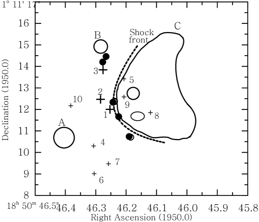
Figure 1: Schematic representation of the G34.3$+$0.15 region. The crosses show the positions of clusters of H₂O masers (the large crosses show the main H₂O clusters), and the circles the positions of the main OH emission regions.

According to the VLA observations of Fey et al. [4], there are three separate groups of H₂O maser spots in a $50^{\prime\prime}\times 30^{\prime\prime}$ area in the G34.3$+$0.15 complex. The largest number of maser spots coincides with the hot core of the molecular cloud, i.e., they are directly connected to the cometary-type HII region (component C). Two other groups of maser spots are separated from the hot core by $20^{\prime\prime}$ and $45^{\prime\prime}$; these are not associated with any continuum source. Their velocities do not differ strongly from those of the spots in the hot core. The H₂O maser spots associated with component C (the cometary HII region) form several clusters [5]. The three main clusters are extended in the radial direction relative to the center of the HII region.

Figure 2: Catalog of spectra of the H₂O maser emission toward G34.3$+$0.15. The double arrow shows the value corresponding to a division of the vertical axis. The radial velocity is given with respect to the LSR.

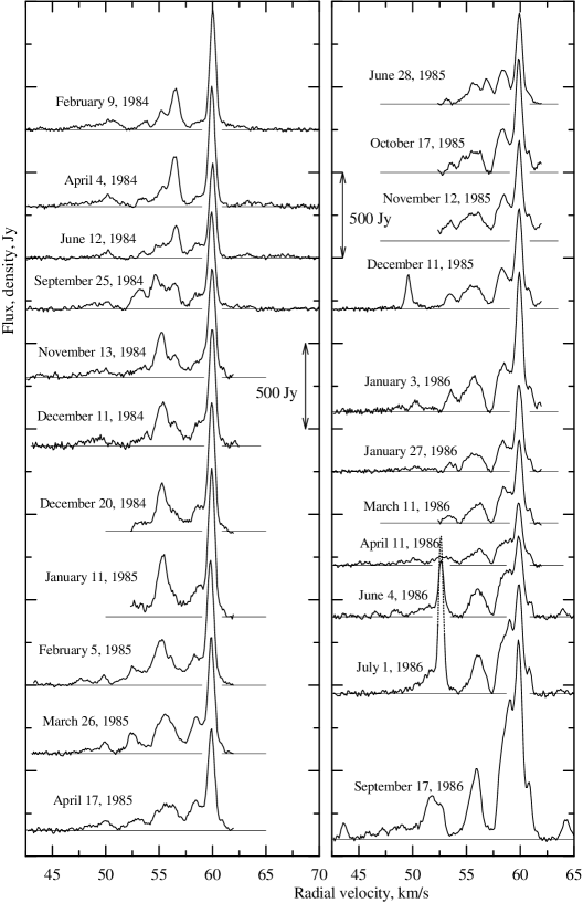
Figure 2: (Contd.)

Figure 2: (Contd.)

Figure 2: (Contd.)

Figure 2: (Contd.)

Figure 2: (Contd.)

Figure 2: (Contd.)

Figure 2: (Contd.)

Figure 2: (Contd.)

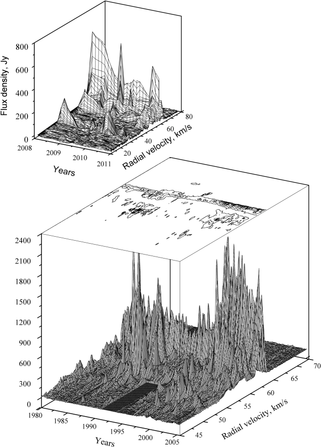
Figure 3: Three-dimensional representation of the catalog of H₂O maser spectra in G34.3$+$0.15.

Figure 4: Superposition of H₂O emission spectra for various time intervals (indicated on the graphs) and for the entire monitoring time (lower right-hand graph). All spectra are given on the same scale.

Figure 5: Spectra of OH maser emission in the 1665 and 1667 MHz lines for left-circular (L) and right-circular (R) polarizations for various observing epochs. The spectral resolution was 1 km/s on January 17 and 29, 1975; 0.138 km/s on January 6, 2008; and 0.068 km/s in 2010.

Figure 6: Stokes parameters for the 1665 and 1667 MHz OH emission on February 25, 2010.

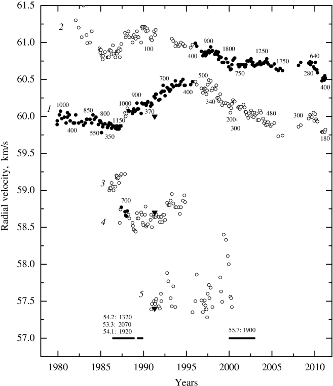
Figure 7: Evolution of H₂O emission features of the main cluster in the radial velocity-interval 57.2–61.2 km/s. The filled circles show features with the greatest flux densities at the corresponding observing epochs, and open circles features for the remaining epochs. Flux densities are given along the graphs of the evolution of features 1 and 2. The triangles show the positions of the emission features observed with the VLA by Fey et al. [4]. The horizontal line segments show the time intervals for strong flares at velocities of 53–56 km/s; the parameters of the flares (radial velocities in km/s and flux densities in janskys) are given.

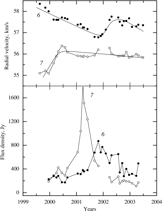
Figure 8: Evolution of the main H₂O emission features of cluster 2 during the flare of 2000–2002. The radial-velocity Variations are approximated by curves.

Figure 9: Evolution of the 1665 and 1667 MHz OH emission in W44C in 1970–2010 (data of [6–9, 14, 16, 21–23] and our observations on the Nançay radio telescope in 1975 and 2008–2010, open symbols).

Subsequent interferometric observations (see, e.g., [6–9]) showed that the H₂O and OH masers are arranged along a parabolic arc near the front of a bow shock at the eastern edge of the cometary HII region. The OH masers are closer to the edge of the cometary region than the H₂O masers, suggesting that the OH molecules are formed via the dissociation of H₂O molecules in the shock; the OH masers probably trace the position of a strong shock that separates the cool molecular cloud from a dense warm envelope encompassing the bow shock [9].

According to the 13-year (1987–1999) observations of Valdettaro et al. [10], there was fairly stable H₂O emission at a radial velocity of about 60 km/s, together with short-lived strong flares at other velocities. In addition, the integrated flux varied by at most a factor of three.

The observations in molecular lines, e.g., C³⁴S [11], ¹³CO, CS, and CH₃CN [12] revealed in this region the presence of a strong north–south radial-velocity gradient on a scale of $\sim 40^{\prime\prime}$. This testifies to the existence of a flow of molecular material in this direction. The velocity gradient was also detected from observations in the H93$\alpha$ recombination line [13].

We first observed W44C in all four 18-cm lines of the OH molecule on the Large radio telescope in Nançay (France) in 1974 [14]. W44C was also observed in the OH lines on the Nançay radio telescope at various later epochs. Since 1979, regular observations (monitoring) of W44C in the H₂O line has been carried out on the 22-m radio telescope in the Pushchino Radio Astronomy Observatory [15].

2 OBSERVATIONS AND DATA

The observations of the H₂O maser emission in the 1.35-cm line toward G34.3$+$0.15 were carried out on the 22-m radio telescope RT-22 in Pushchino from November 1979 to March 2011. The mean interval between observations was less than two months. The noise temperature of the system, with had a cooled FET front-end amplifier, was 150–250 K. An upgrade of the receiver in 2000 lowered the system noise temperature to 100-150 K, depending on weather conditions.

The signal analysis was carried out using a 96-channel (128-channel since July 1997) filter-bank spectrum analyzer with a resolution of 7.5 kHz (0.101 km/s in radial velocity in the 1.35-cm line). A 2048-channel autocorrelator with a resolution of 6.1 kHz (0.0822 km/s at 22 GHz) was used starting at the end of 2005. For a pointlike source, an antenna temperature of 1 K corresponds to a flux density of 25 Jy.

OH-line observations of W44C at 18 cm were conducted on the Large radio telescope of the Nançay Radio Astronomy Station of the Paris–Meudon Observatory (France) at various epochs. The telescope is a Kraus system two-mirror instrument that is able to observe radio sources near the meridian. Using a spherical mirror enables tracking of a radio source by moving the feed within $\pm 30^{\textrm{m}}/\cos\delta$ in hour angle relative the meridian. At declination $\delta=0^{\circ}$ the telescope beam at 18 cm is $3.5^{\prime}\times 19^{\prime}$ in right ascension and declination, respectively. The telescope sensitivity at $\lambda=18$ cm and $\delta=0^{\circ}$ is 1.4 K/Jy. The noise temperature of the helium-cooled front-end amplifiers is 35–60 K, depending on the observing conditions.

The spectral analysis was carried out using an 8192-channel autocorrelator spectrum analyzer. These channels can be divided into several batteries, each realizing an independent signal analysis in one of the two main OH lines (1665 and 1667 MHz) in one of four polarization modes. In our observations in 2008–2009, the spectrum analyzer was divided into eight batteries of 1024 channels each. The frequency bandwidth for each battery was 781.25 kHz, and the frequency resolution 763 Hz. In the 1665 and 1667 MHz lines, this corresponds to a radial-velocity resolution of 0.137 km/s. In the 2010 observations, the resolution was twice as good, 0.068 km/s.

A recent upgrade extended the capabilities for polarization studies [16]. Our 2008–2011 Observations appreciably supplement previous polarization measurements obtained using the Nançay radio telescope. The radio telescope simultaneously receives two perpendicular of linear polarization, which directly yield the intensities of the corresponding linear modes (L$0^{\circ}$, L$90^{\circ}$). Mixing of the signals from the perpendicular feeds with a phase delay of one quarter of a wavelength yields two orthogonal circular-polarization modes (LC, RC). Thus, the three Stokes parameters $I$, $V$, and $Q$ are actually observed simultaneously (with an appropriate choice of coordinate system). The Stokes parameter $U$ can be measured after rotation of the linear-polarization feeds by $45^{\circ}$.

Combining the polarization modes, we can derive all four Stokes parameters of the OH maser emission. The Stokes parameters are determined via the flux densities $F$ of the different polarizations in each frequency channel of the spectrum analyzer as follows [16]:

$$I=F(0^{\circ})+F(90^{\circ})=F(\textrm{RC})+F(\textrm{LC}),$$

$$Q=F(0^{\circ})-F(90^{\circ}),$$

$$U=F(45^{\circ})-F(-45^{\circ}),$$

$$V=F(\textrm{RC})-F(\textrm{LC}).$$

The degree of linear polarization is defined as

$$m_{\mathrm{L}}=\frac{\sqrt{Q^{2}+U^{2}}}{I},$$

the position angle of the linear polarization is

$$\chi=\frac{180^{\circ}}{\pi}\textrm{arctan}\,\left(\frac{U}{Q}\right)$$

and the degree of circular polarization is

$$m_{\mathrm{C}}=\frac{V}{I}.$$

The observational data were processed using the GILDAS software package (IRAM, Grenoble, France), which is available at the address http://www.iram.fr/IRAMFR/GILDAS/. In the processing, we took into account the effects of “spurious” polarization due to signal leakage from one linear-polarization channel to the other. The technique used is described in [17].

Figure 2 presents a catalog of H₂O spectra for the period from November 1979 to March 2011. Observations were not conducted for technical reasons from March 2006 to December 2007. The double arrow shows the value of a division of the vertical axis in janskys. The horizontal axis plots the velocity with respect to the Local Standard of Rest (LSR). For convenience, zero baselines are drawn in the spectra. All the spectra are shown on the same radial-velocity scale.

The catalog of the spectra is also shown as a three-dimensional (3D) graph plotting velocity, time, and flux density (Fig. 3). Constructing a 3D image requires a uniform grid in the velocity–time plane. Velocity intervals are identical, but time intervals are not, since the observations were not equally spaced in time. A more uniform grid was obtained by introducing additional spectra via a linear interpolation. The bottom graph presents the 3D map for 1980–2005 with a resolution of 0.101 km/s, and the top graph the 3D map for 2008–2010 with a resolution of 0.0822 km/s.

Figure 4 presents superpositions of the H₂O spectra for various time intervals and for the total observations time. The separation was determined by the evolution of the spectra. The intervals are indicated on each plot.

H₂O maser emission is observed within several distinct spectral intervals: below 51.6 km/s, 51.6–55.0, 55.0–57.9, 57.9–61.7 km/s, and above 61.7 km/s. The boundaries between them are determined by a pronounced minimum of emission at these velocities, shown by the vertical arrows on the last plot. The most stable emission was observed at 59–61.4 km/s.

The results of the OH-maser observations in the 1665 and 1667 MHz lines at various epochs are shown in Fig. 5. The observations were carried out with a resolution of 1 km/s in 1975, 0.137 km/s in 2008, and 0.068 km/s in 2010. The solid and dashed lines show the emission in the left-circular and right-circular polarization, respectively. The observing technique is described in [18].

The OH emission was essentially constant from 2008 to 2010. Therefore, we present the Stokes parameters $I$, $Q$, $U$, and $V$ only for the observations with a higher spectral resolution carried out on February 25, 2010 (Fig. 6).

3 DISCUSSION

Our analysis of the evolution of the H₂O maser emission during the 30 years of our monitoring has also considered spectra obtained on other radio telescopes and results of observations with a high angular resolution.

3.1 Identification of the Most Stable H₂O Maser Emission Features

Using the VLA observations of Fey et al. [4] and Hofman and Churchwell [5], we have identified main emission features in our monitoring spectra for epochs close to the VLA observations. No interferometric observations of the H₂O maser source in G34.3$+$0.15 were carried out during the period of high maser activity, complicating the identification of some strong flares. Furthermore, due to the low spectral resolution of the VLA observations of Fey et al. [4] (1.3 km/s), not all emission features are present in their maps. For instance, the feature responsible for the emission at 61.3 km/s, which was observed by us throughout almost all of our monitoring, is absent from the VLA images. If this emission belonged to a cluster other than feature 1, it would certainly have been detected by Fey et al. [4].

The most stable H₂O emission in W44C, observed at radial velocities of 59.6–61.5 km/s is identified with the main group of maser spots in W44C—cluster 1 [4, 5] (Fig. 1). Figure 7 shows the evolution of the main emission features of this cluster at radial velocities of 57.2–61.2 km/s. The filled circles show the features whose fluxes were highest at the corresponding observing epochs, while open circles show the remaining epochs. In 1998–2003, feature 1 was appreciably weaker than feature 2. Fluxes are given along the curves for the evolution of features 1 and 2. The triangles mark the positions of emission features from the VLA observations of Fey et al. [4]. The horizontal line segments show time intervals when strong flares occurred at radial velocities of 53–56 km/s; the parameters of these flares (radial velocities and fluxes) are given.

Features 1–3 are arranged radially with respect to the central star in W44C, in order of increasing radial velocity [4]. Some other emission features are identified with clusters of maser spots 2, 3, and 9 (Fig. 1), which are also located near the shock front.

3.2 Long-Term Evolution of the H₂O Maser

The position of the peak of the main emission of cluster 1 varied from 59.5 to 60.5 km/s in a complicated manner. Valdettaro et al. [10] showed that this emission is fairly stable. Our 30-year monitoring likewise indicates this emission to be stable, in the sense that it was observed throughout our monitoring. However, its evolution was complex. We have selected several components. The main ones (1 and 2) were observed throughout our monitoring, with the exception of 1979–1981 for feature 2. The intensity of each component separately varied fairly strongly: by about a factor five for feature 1 and by more than a factor of 20 for feature 2. The variations of the integrated flux of these features were considerably smaller. Thus, we may consider the H₂O maser emission source W44C to be fairly stable.

The highest activity of the H₂O maser took place in 1987–1988 and in 2001. This activity was minimum in 1980, 1992, and 2009, and the minima were more spread out in time than the maxima. Nevertheless, we suggest that the maxima alternated with an interval of 14 years and minima with intervals of 11.5 and 17.5 years. A formal calculation of the mean period of the integrated-flux variability yields a value of $\sim 14$ years.

3.3 H₂O Flare Emission

Flares of individual emission features occurred fairly frequently. However, strong flares (series of flares) exceeding 800 Jy were observed in only three time intervals (Fig. 4), at velocities of 52–57 km/s.

In the first interval (1986–1988) the flux density in flares reached 1800 Jy. At that time, the structure of the entire line profile changed, while the emission of the main components, 1 and 2, was preserved. It is important that, after the first series of flares, the radial-velocity drift of component 2 was small. The drift of component 1 is approximated well by a sine wave within 0.7 km/s. The main components of the flare are identified with the main cluster 1. All this could indicate a global character of the activity of the H₂O maser in W44C.

The flares in 2000–2002 were less prolonged. This emission is most likely identified with another cluster (cluster 2). The flux density in one of the flares reached 1900 Jy. At that time, no structural changes of the main emission of cluster 1 (velocity or flux density) took place. The flares probably had a local character, but occurred during a period of high activity of the entire maser source. The radial-velocity and fluxes variations of the two main components of this flare are shown in Fig. 8. The radial-velocity drift in the local rest frame is complex, and is approximated well by the fitted curves. An approach and subsequent recession of the features in the spectrum can be clearly traced.

Some weaker and shorter flares occurred during the monitoring, in a fairly broad interval of radial velocities.

The observed variability of the components could be a consequence of turbulent motions of matter on scales comparable to the size of maser spots and clusters of maser spots.

3.4 OH Emission

Owing to its one unpaired electron, the OH molecule has a large magnetic dipole moment, 1.66 Debye [19]. Therefore, the observed OH lines spectrum is strongly influenced by an external magnetic field. In a magnetic field, the main lines at 1665 and 1667 MHz split into three components: an unshifted ${\pi}$ component with linear polarization and two ${\sigma}$ components displaced upward and downward in frequency and elliptically polarized in opposite directions. In a longitudinal field with intensity $B$, the frequency separation between the ${\sigma}$ components is

$$\Delta\nu=\frac{5}{2}\frac{g_{J}\mu_{0}}{h}B$$

for the 1665 MHz line and

$$\Delta\nu=\frac{3}{2}\frac{g_{J}\mu_{0}}{h}B$$

for the 1667 MHz line, where $g_{J}$ is the Landé factor (0.935 for both lines), $\mu_{0}$ is the Bohr magneton, $h$ is Planck’s constant, $\mu_{0}/h=1.39967$ kHz/mG, and the separation of the $\sigma$ components in radial velocity is 0.590 km/(s mG) for the 1665 MHz line and 0.354 km/(s mG) for the 1667 MHz line [20].

Measuring the velocity difference of the oppositely polarized ${\sigma}$ components, we can determine the intensity of the longitudinal component of the magnetic field. The positions of the masers of a Zeeman pair on maps measured in the different polarizations coincide to within the errors (for the VLBI measurements, to within fractions of a millisecond). This condition follows from the nature of Zeeman splitting: both ${\sigma}$ components are radiated by each molecule simultaneously as a result of its precession in the magnetic field. VLBI observations of masers confirm that there is indeed positional coincidence of the ${\sigma}$ components, though their intensities are usually not equal. Basically, the total or partial suppression of one ${\sigma}$ component by the other is possible. In this case, only one $\sigma$ component with a high degree of circular polarization (up to 100%) is observed.

The general profile of the 1665 and 1667 MHz OH lines toward source C is formed mainly by emission from the regions near the main clusters of H₂O spots, namely, 1, 2, and 3. Thus, the most intense H₂O and OH maser emission arises in spatially nearby regions. As was noted in the Introduction, the most intense OH sources are located just upstream of the ionization front of the HII region W44C [6, 7].

Figures 5–6 present our 1665 and 1667 MHz OH lines data obtained on the Nançay radio telescope. Figure 99 shows the evolution of the 1665 and 1667 MHz emission in W44C in 1970–2010 according to [6–9, 14, 16, 21–23] and our own Nançay observations in 1974, 1975 and 2008–2010. Since the onset of OH line observations of W44C [21], the peak flux density of the most intense feature in the 1667 MHz line, at 58 km/s, has increased by more than an order of magnitude. The flux density in the 1665 MHz line has also increased. One peculiarity of W44C that distinguishes it from other OH masers in star-forming regions is the greater intensity of the 1667 MHz line as compared to the 1665 MHz line. In the majority of masers of this class, the 1665 MHz line is more intense than the 1667 MHz line. This difference may be related to the particulars of the OH maser pumping in W44C near the shock front of the cometary HII region.

4 MAIN RESULTS

Let us summarize the main results obtained from our 30-year monitoring of the water maser and long-term monitoring of the hydroxyl maser in G34.3$+$0.15.

1. We present here a catalog of H₂O maser spectra in the 1.35 cm line toward G34.3$+$0.15 for the period from November 1979 to March 2011 (Fig. 2), with a mean interval between observational sessions of about two months. The radial-velocity resolution was 0.101 km/s before and 0.0822 km/s after the end of 2005.

2. We have found an alternation of maxima and minima of the H₂O maser activity. A formal calculation of the mean period of activity yields $\sim 14$ years; however, this is consistent with our results for a number of other sources associated with regions of active star formation.

3. We have observed two series of strong flares of the H₂O maser emission, also with an interval of 14 years, which were associated with two different clusters of maser spots (1 and 2) localized at the shock front at the periphery of the ultracompact region UH II. These series of flares took place during periods of enhanced maser activity, and are probably related to cyclic activity of the protostellar object in UH II (component C). In the remaining time intervals, there were mainly short-lived flares of single features.

4. The observed character of the variability of the emission of individual H₂O maser components may be a consequence of turbulent (including vortical) motions of matter, within maser spots and clusters of spots located near the shock front.

5. Since the discovery of OH emission in W44C at the beginning of the 1970, the flux density of the OH lines has gradually increased, and has currently reached a maximum for the entire time covered by observations. This increase could be related to the propagation of a shock exciting maser emission deep within the molecular cloud.

6. We have estimated the intensity of the line-of-sight magnetic field to be –1.2mG from the splitting of the 1667 MHz OH maser feature at 58.6 km/s. The field is directed toward the observer, consistent with the general pattern of the magnetic field in the W44C region mapped by interferometric observations [9].

References

- [1] M. J. Reid and P. T. P. Ho, Astrophys. J. 288, 417 (1985).
- [2] D. O. S. Wood and E. Churchwell, Astrophys. J. Suppl. Ser. 69, 831 (1989).
- [3] B. E. Turner and R. H. Rubin, Astrophys. J. 170, L113 (1971).
- [4] A. L. Fey, R. A. Gaume, G. E. Nedoluha, and M. J. Claussen, Astrophys. J. 435, 738 (1994).
- [5] P. Hofner and E. Churchwell, Astron. and Astrophys. Suppl. Ser. 120, 283 (1996).
- [6] A. L. Argon, M. J. Reid, and K. M. Menten, Astrophys. J. Suppl. Ser. 129, 159 (2000).
- [7] X. Zheng, J. M. Moran, and M. J. Reid, Monthly Not. Roy. Astron. Soc. 317, 192 (2000).
- [8] X. Zheng, M. J. Reid, and J. M. Moran, Astron. and Astrophys. 357, L37 (2000).
- [9] N. Gasiprong, R. J. Cohen, and B. Hutawarakorn, Monthly Not. Roy. Astron. Soc. 336, 47 (2002).
- [10] R. Valdettaro, F. Palla, J. Brand, et al., Astron. and Astrophys. 383, 244 (2002).
- [11] R. Cesaroni, C. M. Walmsley, C. Kömpe, and E. Churchwell, Astron. and Astrophys. 252, 278 (1991).
- [12] E. Churchwell, C. M. Walmsley, and D. O. S. Wood, Astron. and Astrophys. 253, 541 (1992).
- [13] R. A. Gaume, A. L. Fey, and M. J. Claussen, Astrophys. J. 432, 648 (1994).
- [14] M. I. Pashchenko, Sov. Astron. Lett. 1, 241 (1975).
- [15] E. E. Lekht, M. I. Pashchenko, G. M. Rudnitskiĭ, and R. L. Sorochenko, Sov. Astron. 26, 168 (1982).
- [16] M. Szymczak and E. Gérard, Astron. and Astrophys. 423, 209 (2004).
- [17] V. I. Slysh, M. I. Pashchenko, G. M. Rudnitskiĭ, et al., Astron. Reports 54, 599 (2010).
- [18] M. I. Pashchenko, G. M. Rudnitskiĭ, and P. Colom, Astron. Reports 53, 541 (2009).
- [19] A. A. Radtsig and B. M. Smirnov, Handbook of Atomic and Molecular Physics (Moscow: Atomizdat, 1980). In Russian.
- [20] R. D. Davies, in: Galactic Radio Astronomy, Proc. IAU Symp. No. 60, Maroochydore, Queensland, Australia, 3–7 September 1973, eds F. J. Kerr, S. C. Simonson (Dordrecht, Holland–Boston: Reidel, 1974), p. 275.
- [21] B. E. Turner, Astron. and Astrophys. Suppl. Ser. 37, 1 (1979).
- [22] J. L. Caswell and R. F. Haynes, Austral. J. Phys. 36, 417 (1983).
- [23] R. A. Gaume and R. L. Mutel, Astrophys. J. Suppl. Ser. 65, 193 (1987).