Adopting the framework of two-coupled superconducting charges model, we discussed the information entropy of two qubits initially prepared in a mixed state and allowed to interact with their environment. The impact of the different parameters of the system is explicitly investigated. Present calculations show that a strong mutual entropy is obtained for a long interaction time when the two qubits are initially in a mixed state with the environment switched off. We have identified a class of two-qubit states that have a rich dynamics when the deviation between the characteristic energies of the qubits become minimum. It was found that the total correlation decreases abruptly to zero in a finite time due to the influence of the strong environment.

PACS: 32.80.-t; 42.50.Ct; 03.65.Ud; 03.65.Yz.

1 Introduction

In designing and analyzing cryptosystems and protocols, mathematical concepts are critical in supporting the claim that the intended cryptosystem is secure [1] and different concepts have important impact in this direction, e.g. the pseudo entropy as a measure of information content of ionic state due to ion-laser interaction in a single trapped ion has been used [2] superconductor-based quantum information processor [3], and optical properties of quantum charge qubits structures are currently in the focus of the research activity owing to their promising potentiality in different areas of present-day science and technology [4, 5]. One of the physical realizations of a solid-state qubit is provided by a Cooper pair box which is a small superconducting island connected to a large superconducting electrode, a reservoir, through a Josephson junction [6]. Superconducting charge qubits (Cooper pair boxes) are a promising technology for the realization of quantum computation on a large scale [7, 8, 9, 10].

On the other hand, one of the major challenges in the field of quantum information theory is to get a deep understanding of how local operations assisted by classical communication performed on a multi-level quantum system can affect the entanglement between the spatially separated systems. Despite a lot of progress in the last few years, it is still not fully understood. For instance, even for the simple question of whether a given state is entangled or not, no general answer is known [11]. An interesting question raised in [12] is whether there is any relationship between the uncertainty principle and entanglement or not. Recently, a general definition of entropy squeezing for a two-level system has been presented [13] and showed that the information entropy is a measure of the quantum uncertainty of atomic operators. Also, the number-phase entropic uncertainty relation for the multiphoton coherent state and nonlinear coherent state is studied and compared with an ordinary coherent state [14].

The purpose of this paper is to propose the quantum mutual entropy as a measure of the total correlation between two-coupled superconducting charge qubits, each qubit is based on a Cooper pair box connected to a reservoir electrode through a Josephson junction. Our approach in relating the correlation of the pair of two charge qubits system to the maximum entangled state generated has the merit of directly involving quantities having a clear physical meaning. Applying our criterion to the considered system we are able to fully exploit the novelty of our point of view to explain the ability to generate maximum entangled states and the corresponding correlation.

This paper is organized as follows: in Section 2, we will describe the Hamiltonian of the system of interest, and obtain the explicit analytical solution of the master equation describing the dynamics of two qubits in the presence of phase decoherence. In Section 3, we discuss the total correlation of the system by virtue of the mutual entropy in the absence or presence of the decoherence. Finally, Section 4 presents the conclusions and an outlook.

2 The model

We consider two charge qubits and couple them by means of a miniature on-chip capacitor [9, 15]. The read-out of each qubit, in this case, is done similar to the single qubit read-out and connect a probe electrode to each qubit. External controls that we have in the circuit are the dc probe voltages $V_{b_{1}}$ and $V_{b_{2}}$, $d_{c}$ gate voltages $V_{g_{1}}$ and $V_{g_{2}}$, and pulse gate voltage $V_{p}$. The information on the final states of the qubits after manipulation comes from the pulse-induced currents measured in the probes. By doing routine current– voltage–gate voltage measurements, we can estimate the capacitances. We then perform state manipulation and demonstrate qubit–qubit interaction. The Hamiltonian of the system in the charge representation can be written as [9]

$$\hat{H} = \hbar\sum_{n_{1}=0}^{\infty}\sum_{n_{2}=0}^{\infty}\eta_{1}(n_{1},n_{2})|n_{1},n_{2}\rangle\langle n_{1},n_{2}|$$

$$-\frac{E_{J_{1}}}{2}\left(|n_{1},n_{2}\rangle\langle n_{1}+1,n_{2}|+|n_{1},n_{2}+1\rangle\langle n_{1}+1,n_{2}+1|\right)$$

$$-\frac{E_{J_{2}}}{2}\left(|n_{1},n_{2}\rangle\langle n_{1},n_{2}+1|+|n_{1}+1,n_{2}\rangle\langle n_{1}+1,n_{2}+1|\right),$$

The parameter $\eta_{1}(n_{1},n_{2})=E_{c_{1}}\left(n_{g_{1}}-n_{1}\right)^{2}+E_{c_{2}}\left(n_{g_{2}}-n_{2}\right)^{2}+E_{m}\left(n_{g_{1}}-n_{1}\right)\left(n_{g_{2}}-n_{2}\right).$ Here, $n_{1}$ and $n_{2}$ ($n_{1},n_{2}=0,\pm 1,\pm 2,...$) define the number of excess Cooper pairs in the first and the second Cooper pair boxes respectively, and $n_{g_{1,2}}=(C_{g_{1,2}}V_{g_{1,2}}+C_{p}V_{p})/2e$ are the normalized charges induced on the corresponding qubit by the $d_{c}$ and pulse gate electrodes. The eigenenergies, $E_{k}$ $(k=0,1,2,...$), of the Hamiltonian in (2) form $2e$-periodic energy bands corresponding to the ground ($k=0$), first excited ($k=1$), etc. states of the system. The energy bands $E_{k}$ for the one-dimensional case were first introduced in Ref. [9, 15]. $E_{c_{1}}$, $E_{c_{2}}$ and $E_{m}$ give the characteristic energies of Cooper pair of the first qubit, Cooper pair charging energy of the second qubit and the coupling energy, respectively. $E_{c1,2}=\frac{4e^{2}C_{\varepsilon 2,1}}{2(C_{\varepsilon 1}C_{\varepsilon 2}-C_{m}^{2})},$ and $E_{m}=\frac{4e^{2}C_{m}}{C_{\varepsilon 1}C_{\varepsilon 2}-C_{m}^{2}},$where $C_{\varepsilon_{2,1}}$ are the sum of all capacitances connected to the corresponding Cooper pair box including the coupling capacitance $C_{m}$ and $e$ is the electron charge.

If the circuit is fabricated to have the following relation between the characteristic energies: $E_{J_{1,2}}\sim$ $E_{m}<E_{c_{1,2}}$, then one can use a four-level approximation for the description of the system ($|e_{1}e_{2}\rangle,|g_{1}e_{2}\rangle,|e_{1}g_{2}\rangle$ and $|g_{1}g_{2}\rangle$) around $n_{g_{1}}=n_{g_{2}}=0.5$ while other charge states are separated by large energy gaps. These four charge states can be used as a new basis for the Hamiltonian (2).

Decoherence is not always due to the interaction with an environment, but it may also be due, to the fluctuations of some classical parameter or internal variable of a system. This is a different form of decoherence, which is present even in isolated systems which is called non-dissipative decoherence. In this paper, we follow the standard procedure [16, 17, 18] to write the time evolution of the system density operator $\hat{\rho}(t)$ in the following form

$$\frac{d}{dt}\hat{\rho}(t)=-\frac{i}{\hbar}[\hat{H},\hat{\rho}]-\frac{\gamma}{2\hbar^{2}}[\hat{H},[\hat{H},\hat{\rho}]],$$ (2)

where $\gamma$ is the phase decoherence rate. Equation (2) reduces to the ordinary von Neumann equation for the density operator in the limit $\gamma\rightarrow 0.$ The equation with the similar form has been proposed to describe the intrinsic decoherence [19]. Under Markov approximations the  solution of the master equation can be expressed as follows

$$\rho(t)=\left(\begin{array}[]{c}\rho_{ee,ee}\\ \rho_{eg,ee}\\ \rho_{ge,ee}\\ \rho_{gg,ee}\end{array}\begin{array}[]{c}\rho_{ee,eg}\\ \rho_{eg,eg}\\ \rho_{ge,eg}\\ \rho_{gg,eg}\end{array}\begin{array}[]{c}\rho_{ee,ge}\\ \rho_{eg,ge}\\ \rho_{ge,ge}\\ \rho_{gg,ge}\end{array}\begin{array}[]{c}\rho_{ee,gg}\\ \rho_{eg,gg}\\ \rho_{ge,gg}\\ \rho_{gg,gg}\end{array}\right).$$ (3)

We use the notation $|ij\rangle=|i_{1}\rangle\otimes|j_{2}\rangle,$ $(i,j=e,g),$ where $|e_{1(2)}\rangle$ and $|g_{1(2)}\rangle$ are the basis states of the first (second) qubits and $\rho_{ij,lk}(t)=\langle ij|\rho(t)|lk\rangle$ corresponds the diagonal ($ij=lk$) and off-diagonal ($ij\neq lk)$ elements of the final state density matrix $\rho(t).$ From here on, for tractability of notation and without loss of generality, we denote by $\rho_{ij}(t)=\rho_{ij,ij}(t),$ the probability of finding the two-coupled qubits in the charge state $|ij\rangle.$

3 Information entropy

In the theory of open system or the reduction theory, one often considers two subsystem $\mathcal{H}_{1}$ and $\mathcal{H}_{2}$ represented by Hilbert space. Let $\mathfrak{S}(\mathcal{H}_{i}),\,\,(i=1,2)$ be state spaces (the set of all density operators). Also $\mathfrak{S}(\mathcal{H}_{1}\otimes\mathcal{H}_{2})$ denotes the state space in the composite system $\mathcal{H}_{1}\otimes\mathcal{H}_{2}$ [20]. The following decomposed states in composite system are called disentangled states :

$$|\Psi\rangle=|\psi_{1}\rangle\otimes|\psi_{2}\rangle,{\ \ \ \ \ \ }|\psi_{1}\rangle\in\mathfrak{S}(\mathcal{H}_{1}),{\ \ \ \ \ \ }|\psi_{2}\rangle\in\mathfrak{S}(\mathcal{H}_{2}).$$ (4)

However in general it is almost impossible to decompose the states in composite system like the above, that is, the following states exist :

$$|\Psi\rangle = \alpha|\psi_{1}\rangle\otimes|\psi_{2}\rangle+\beta|\phi_{1}\rangle\otimes|\phi_{2}\rangle,$$ (5)

$$|\psi_{1}\rangle,{\ \ \ }|\phi_{1}\rangle\in\mathfrak{S}(\mathcal{H}_{1}),\,\qquad\,|\psi_{2}\rangle,{\ \ \ \ }|\phi_{2}\rangle\in\mathfrak{S}(\mathcal{H}_{2})$$

$$|\alpha|^{2}+|\beta|^{2}=1,{\ \ \ \ \ \ \ \ }\alpha\neq 0,{\ \ \ \ \ \ }\beta\neq 0.$$

The above states which can not be described by product states of two subsystem, are called entangled states. For the entangled states $\mathcal{E}_{t}^{\ast}\rho\in\mathfrak{S}(\mathcal{H}_{1}\otimes\mathcal{H}_{2})$, the quantum mutual entropy is defined by the following formula as a distance (difference) from a disentangled state $tr_{\mathcal{H}_{1}}\varrho\otimes tr_{\mathcal{H}_{2}}\varrho\in\mathfrak{S}(\mathcal{H}_{1}\otimes\mathcal{H}_{2})$

$$I_{\mathcal{E}_{t}^{\ast}\rho}\left(\rho^{A},\rho^{B}\right)=tr\mathcal{E}_{t}^{\ast}\rho(\log\mathcal{E}_{t}^{\ast}\rho-\log(tr_{\mathcal{H}_{1}}\mathcal{E}_{t}^{\ast}\rho\otimes tr_{\mathcal{H}_{2}}\mathcal{E}_{t}^{\ast}\rho)).$$ (6)

Note that if the entangled state $\mathcal{E}_{t}^{\ast}\rho$ is a pure state, $S(\mathcal{E}_{t}^{\ast}\rho)=0$ and then $S(tr_{\mathcal{H}_{2}}\mathcal{E}_{t}^{\ast}\rho)=S(tr_{\mathcal{H}_{1}}\mathcal{E}_{t}^{\ast}\rho)$ by Araki-Lieb inequality [21], thus we have $I_{\mathcal{E}_{t}^{\ast}\rho}\left(\rho^{A},\rho^{B}\right)=2S(tr_{\mathcal{H}_{2}}\mathcal{E}_{t}^{\ast}\rho)$.

We now suppose that the initial state of the Cooper pairs is a mixed state:

$$\rho=\cos^{2}\left(\frac{\xi}{2}\right)\left|e_{1}e_{2}\right\rangle\langle e_{1}e_{2}|+\sin^{2}\left(\frac{\xi}{2}\right)\left|g_{1}g_{2}\right\rangle\langle g_{1}g_{2}|.$$ (7)

In what follows, we are going to derive a general form of the quantum mutual entropy $I_{\mathcal{E}_{t}^{\ast}\rho}\left(\rho^{A},\rho^{B}\right)$ for two charge qubits. Using equations (LABEL:fdens) and (7), one can write the von-Neumann entropy of the two-qubit state as

$$S(\mathcal{E}_{t}^{\ast}\rho)=-\sum_{i=1}^{4}\lambda_{i}^{(AB)}(t)\log_{2}\lambda_{i}^{(AB)}(t),$$ (8)

where $\lambda_{1}^{(AB)}(t)=\langle e_{1}e_{2}|\mathcal{E}_{t}^{\ast}\rho|e_{1}e_{2}\rangle,$ $\lambda_{2}^{(AB)}(t)=\langle g_{1}g_{2}|\mathcal{E}_{t}^{\ast}\rho|g_{1}g_{2}\rangle,$

$$\lambda_{3,4}^{(AB)}(t) = \frac{\langle e_{1}g_{2}|\mathcal{E}_{t}^{\ast}\rho|e_{1}g_{2}\rangle+\langle g_{1}e_{2}|\mathcal{E}_{t}^{\ast}\rho|g_{1}e_{2}\rangle}{2}$$

$$\pm\frac{1}{2}\sqrt{\left(\langle e_{1}g_{2}|\mathcal{E}_{t}^{\ast}\rho|e_{1}g_{2}\rangle+\langle g_{1}e_{2}|\mathcal{E}_{t}^{\ast}\rho|g_{1}e_{2}\rangle\right)^{2}+4|\langle e_{1}g_{2}|\mathcal{E}_{t}^{\ast}\rho|g_{1}e_{2}\rangle|^{2}}.$$

The von Neumann entropy of reduced density operator of the first qubit $S(\rho_{t}^{A})$ is given

$$S(\rho_{t}^{F})=-\sum_{i=1}^{2}\lambda_{i}^{(A)}(t)\log_{2}\lambda_{i}^{(A)}(t).$$ (9)

where $\lambda_{1}^{(A)}(t)=\langle e_{1}|\rho^{(A)}|e_{1}\rangle,$ $\lambda_{2}^{(A)}(t)=\langle g_{1}|\rho^{(A)}|g_{1}\rangle,$ while the von Neumann entropy of reduced density operator of the second qubit $S(\rho_{t}^{B})$ can be written as

$$S(\rho_{t}^{F})=-\sum_{i=1}^{2}\lambda_{i}^{(B)}(t)\log_{2}\lambda_{i}^{(B)}(t).$$ (10)

where $\lambda_{1}^{(B)}(t)=\langle e_{2}|\rho^{(B)}|e_{2}\rangle,$ and $\lambda_{2}^{(B)}(t)=\langle g_{2}|\rho^{(B)}|g_{2}\rangle.$

Thus we rigorously obtain the analytical expression of the quantum mutual entropy of the system under consideration in the following form (8) and (9)

$$I_{\mathcal{E}_{t}^{\ast}\rho}\left(\rho^{A},\rho^{B}\right) \equiv tr\mathcal{E}_{t}^{\ast}\rho(\log\mathcal{E}_{t}^{\ast}\rho-\log(\rho_{t}^{A}\otimes\rho_{t}^{B}))$$ (11)

$$= S(\rho_{t}^{(A)})+S(\rho_{t}^{(B)})-S(\mathcal{E}_{t}^{\ast}\rho)$$

$$- \sum_{i=1}^{2}\lambda_{i}^{(A)}(t)\log_{2}\lambda_{i}^{(A)}(t)-\sum_{i=1}^{2}\lambda_{i}^{(B)}(t)\log_{2}\lambda_{i}^{(B)}(t)$$

$$+\sum_{i=1}^{4}\lambda_{i}^{(AB)}(t)\log_{2}\lambda_{i}^{(AB)}(t).$$

Throughout this paper, we use the quantum mutual entropy equation (11) as a measure of the total correlation of two qubits. It turns out to be rather easy to derive an analytic expression for the quantum mutual entropy for any given system, since with the help of equation (11) it is possible to study the total correlation of any two-qubit system when the system starts from a mixed state. This measure is not only a function of interaction time but also a function of coupling energy, characteristic energies and initial state setting. We now turn to the task of numerically analyzing the effect of the system parameters on the total correlation and occupation probabilities of the four charge states. It is obvious that correlation does not appear when the coupling energy parameter $E_{m}=0$ because the two qubits state becomes separable and correlation is not generated. For $E_{m}\neq 0$, we found that correlation is produced between the qubits regardless of characteristic energies when the qubits are initially prepared in mixed state and $\gamma=0$ (see Figure 1).

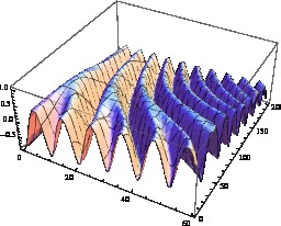
Figure 1: Numerical results for quantum mutual entropy as a function of the scaled time and coupling energy. The parameters used in these figures are $E_{J1}=E_{J2}=30,\gamma=0,$ and the initial state of the two qubits is maximally entangled.

It is shown that the qubits exist between the upper and lower states only with very small probability of being in the intermediate states and maximum entangled mixed states in the form $\rho=\frac{1}{2}\left(\left|e_{1}e_{2}\right\rangle\langle e_{1}e_{2}|+\left|g_{1}g_{2}\right\rangle\langle g_{1}g_{2}|\right)$ is obtained at some instances that corresponding to the maximum correlation, i.e. given enough time, the system will therefore reaches a state where both excited and ground states have equal occupation probabilities. Indeed in the limit that $\theta\sim 0,$ the quantum mutual entropy is only twice of the quantum von Numann entropy. In the general case ($i.e.,$ $\theta\neq 0$), the final state does not necessarily become a pure state, so that we need to make use of $I_{\mathcal{E}_{t}^{\ast}\rho}\left(\rho_{t}^{A},\rho_{t}^{F}\right)$ in the present model. Thus our initial setting enables us to discuss the variation of the quantum mutual entropy for different values of the mixed state parameter $\theta.$ A related model allowing an analytic treatment of the quantum entanglement as well as valuable insight, namely an ensemble of two identical qubits coupled to a cavity field has been discussed in  [22].

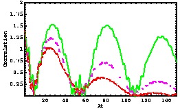
Figure 2: The time evolution of the quantum mutual entropy as a function of the scaled time and different values of the decoherence parameters, where, $\gamma=0.01$ (solid curve), $\gamma=0.1$ (dashed curve), $\gamma=0.5$ (dot curve). The other parameters are the same as figure 1.

Since one of our main goals is to analyze the different possible types of behavior in the coupled qubits dynamics, we have to identify the relevant parameters that determine the different behavior regimes. In Figure 2, we consider the quantum mutual entropy as a function of the scaled time for different values of the decoherence parameter $\gamma$. This case is quite interesting because the quantum mutual entropy function oscillates around the maximum and minimum values for small period of the interaction time and the local maximum decreases as time goes on. We have shown here a new phenomena where the periodic oscillations occur irrespective of the decoherence. A slight change in $\gamma$ therefore, dramatically alters the quantum mutual entropy. It should be noted that for a special choice of the decoherence parameter, the situation becomes interesting where, correlation decreases abruptly to zero in a finite time due to the influence of the strong environment. Nevertheless, the sharp peaks lie within the region between the two maximum values of the correlation occurring in a similar way for different values of the decoherence parameter but the local maximum is decreased, such that with higher $\gamma$ these oscillations of the quantum mutual entropy decay to local minimum which is close to zero. From our further calculations, we notice that if the difference between the two characteristic energies is substantially larger than the coupling energy, the effect of the decoherence on the total correlation dynamics diminishes rapidly. Then, we have emphasized and identified that for some higher values of $\gamma$ there were no persisting periods found to lie between the two maximum values. Similar effects have been observed in different systems experimentally [23] and theoretically [24].

From our further calculations, we see that the time evolution of total correlation for different values of the characteristic energies $E_{J_{1}}$ and $E_{J_{2}}$ when the charge qubits are initially prepared in a mixed state keeping the coupling energy fixed, the number of oscillations of the quantum mutual entropy is increased as the deviation between $E_{J_{1}}$ and $E_{J_{2}}$ is increased while its dynamics exhibits the same qualitative behaviors which has been observed in Figure 1. However, it is interesting to note that when characteristic energies take different values i.e. $E_{J_{1}}\neq E_{J_{2}}$ even with different values of the mixed state parameter $\theta$, the intermediate level always populated and oscillate around small values. Total correlation is maximized when the qubits are initially prepared in a mixed state and the deviation takes its minimum value ($E_{J_{1}}\simeq E_{J_{2}})$. Compared with Figure 1, the long levied maximum correlation is no longer exists in this case and increasing the deviation between the characteristic energies produces more oscillations from the early stage of interaction with sharp peaks of the local maximum of the correlation function. Because of different values of the characteristic energies which are control the qubits, the interaction becomes more complicated and brings about faster oscillations in quantum mutual entropy.

Our quantitative results are of potential use in the analysis of a broad class of relevant experimental situations dealing with quantum information theory. It is worth mentioning that the dynamics of coupled superconducting charges systems has always been of interest, but has recently attracted even more attention because of application in quantum computing. Several systems have been suggested as physical realizations of quantum bits allowing for the needed control manipulations, and for some of them the first elementary steps have been demonstrated in experiments [8].

4 Conclusion

Summarizing, we have analyzed the quantum correlation of a physically interesting system interacting with its environment in the context of two-coupled superconducting charges model. We have explicitly evaluated the exact solution of the density matrix of the system and worked out the effects of different parameters of the system as well as environmental parameter on the dynamics of the system. In particular, a considerable enhancement of maximum entangled mixed state generation of semiconductor qubits is obtained when even weak coupling energy is employed. We have identified the relation between the quantum mutual entropy as a measure of quantum correlation between the two charge qubits and maximum entangled state generation. This seems significant, and one then wonders whether the trend might continue with the general multi-level case. With an increase in exposure to the environment, and for small values of the coupling energy, we found faster decays of the total correlation when the qubits are initially prepared in mixed state. This fast decay rate of quantum correlation is a generic feature in a variety of physical processes where decoherence is important. This kind of numerical investigation constitutes the first quantitative characterization of the relation between the total correlation and maximum entangled state generation for the superconducting charges qubits.

References

- [1] Y. F. Chung, Z. Y. Wub and T. S. Chen, Information Sciences 178 (2008) 2044–2058
- [2] A.-S.F. Obada, S. Furuichi, H.F. Abdel-Hameed and M. Abdel-Aty, Information Sciences 162 (2004) 53–61
- [3] O. Astafiev, Yu. A. Pashkin, Y. Nakamura, T. Yamamoto, and J. S. Tsai, Phys. Rev. Lett. 96, 137001 (2006)
- [4] A. O. Niskanen, K. Harrabi, F. Yoshihara, Y. Nakamura, S. Lloyd, and J. S. Tsai Science, 316, 723 (2007)
- [5] J. Q. You and F. Nori, Physics Today, 58, 42 (2005); J. Q. You, J. S. Tsai, and F. Nori, Phys. Rev. B 73, 014510 (2006)
- [6] E. J. Griffith, C. D. Hill, J. F. Ralph, H. M. Wiseman and K. Jacobs, Phys. Rev. B 75, 014511 (2007)
- [7] K. B. Cooper, M. Steffen, R. McDermott, R. W. Simmonds, S.Oh, D. A. Hite, D. P. Pappas, and J. M. Martinis, Phys. Rev. Lett. 93, 180401 (2004).
- [8] Y. Nakamura, Y. A. Pashkin, and J. S. Tsai, Nature. 398, 786 (1999).
- [9] Yu. A. Pashkin, T. Yamamoto, O. Astafiev, Y. Nakamura, D. V. Averin, T. Tilma, F. Nori and J. S. Tsai, Physica C 426–431 1552 (2005).
- [10] Yu. A. Pashkin, T. Yamamoto, O. Astafiev, Y. Nakamura, D. V. Averin, J. S. Tsai, Nature 421, 823 (2003).
- [11] A. C. Doherty, P. A. Parrilo and F. M. Spedalieri, Phys. Rev. A 69, 022308 (2004)
- [12] O. Guhne and M. Lewenstein, Phys. Rev. A 70, 022316 (2004)
- [13] M. F. Fang, P. Zhou and S. Swain, J. Mod. Opt. 47, 1043 (2000)
- [14] A. Joshi, J. Opt. B: Quantum Semiclass. Opt. 3, 124 (2001)
- [15] D. V. Averin, A.B. Zorin and K. K. Likharev, JETP 61, 407 (1985).
- [16] H.-P. Breuer and F. Petruccione, The theory of open quantum systems, Oxford University Press, Oxford, (2002)
- [17] D. A. Lidar and K. B. Whaley, in Irreversible quantum dynamics edited F.Benatti and R. Floreanini, Spring Lecutre Notes in Physics,Vol. 62, Berlin (2003), p.83.
- [18] C. W. Gardiner and P. Zoller, Quantum Noise (Springer-Verlag, Berlin, 2000).
- [19] G.J. Milburn, Phys. Rev. A 44, 5401 (1991); S. Schneider and G.J. Milburn, Phys. Rev. A 57, 3748 (1998); S. Schneider and G.J. Milburn, Phys. Rev. A 59, 3766 (1999).
- [20] T. Yu and J. H. Eberly, Phys. Rev. Lett. 97, 140403 (2006); ibid Quantum Information and Computation, (2007) in press
- [21] H. Araki and E. Lieb, Commun. Math. Phys. 18, 160 (1970)
- [22] M. Abdel-Aty and A.-S. F. Obada, J. Math. Phys. 45, 4271 (2004)
- [23] M. P. Almeida, F. de Melo, M. Hor-Meyll, A. Salles, S. P. Walborn, P. H. Souto Ribeiro, L. Davidovich, Science, 316, 579 (2007)
- [24] J. H. Eberly and T. Yu, Science, 316, 555 (2007); A.-S. F. Obada and M. Abdel-Aty, Phys. Rev. B, 75, 195310 (2007)