Fundamental properties of five Kepler stars using global asteroseismic quantities and ground-based observations

Abstract

Context. We present an asteroseismic study of the solar-like stars KIC 11395018, KIC 10273246, KIC 10920273, KIC 10339342, and KIC 11234888 using short-cadence time series of more than eight months from the Kepler satellite. For four of these stars, we derive atmospheric parameters from spectra acquired with the Nordic Optical Telescope. The global seismic quantities (average large frequency separation and frequency of maximum power), combined with the atmospheric parameters, yield the mean density and surface gravity with precisions of 2% and $\sim$0.03 dex, respectively. We also determine the radius, mass, and age with precisions of 2–5%, 7–11%, and $\sim$35%, respectively, using grid-based analyses. Coupling the stellar parameters with photometric data yields an asteroseismic distance with a precision better than 10%. A $v\sin i$ measurement provides a rotational period-inclination correlation, and using the rotational periods from the recent literature, we constrain the stellar inclination for three of the stars. An Li abundance analysis yields an independent estimate of the age, but this is inconsistent with the asteroseismically determined age for one of the stars. We assess the performance of five grid-based analysis methods and find them all to provide consistent values of the surface gravity to $\sim$0.03 dex when both atmospheric and seismic constraints are at hand. The different grid-based analyses all yield fitted values of radius and mass to within 2.4$\sigma$, and taking the mean of these results reduces it to 1.5$\sigma$. The absence of a metallicity constraint when the average large frequency separation is measured with a precision of 1% biases the fitted radius and mass for the stars with non-solar metallicity (metal-rich KIC 11395018 and metal-poor KIC 10273246), while including a metallicity constraint reduces the uncertainties in both of these parameters by almost a factor of two. We found that including the average small frequency separation improves the determination of the age only for KIC 11395018 and KIC 11234888, and for the latter this improvement was due to the lack of strong atmospheric constraints.

Aims.

Methods.

Results.

1 Introduction

Stars like the Sun have deep convective envelopes where stochastic excitation gives rise to a rich spectrum of resonant oscillation modes (e.g. Brown & Gilliland 1994; Christensen-Dalsgaard 2005; Aerts et al. 2010). The frequencies of the modes depend on the journey that the waves make through the star, so that if the seismic signatures can be observed, they provide very accurate probes of the stellar interior (Ulrich, 1970; Leibacher & Stein, 1971; Christensen-Dalsgaard, 2007; Metcalfe et al., 2010; Deheuvels & Michel, 2010a; de Meulenaer et al., 2010; Van Grootel et al., 2010; Creevey & Bazot, 2011). The oscillations have tiny amplitudes, and with photometry they can only be revealed with very long high-precision time series from space, e.g. with CoRoT (Baglin, 2003; Appourchaux et al., 2008; García et al., 2009; Mosser et al., 2009; Deheuvels et al., 2010b; Mathur et al., 2010a).

The Kepler satellite (Borucki et al., 2010), which was launched in early 2009, is providing photometric data of outstanding quality on thousands of stars, see e.g. Bedding et al. (2010), Gilliland et al. (2010a), Hekker et al. (2010), Huber et al. (2010), Kallinger et al. (2010), and Stello et al. (2010). With an average cadence of 30 minutes, the primary objectives of the mission, to search for and characterise Earth-like planets, can be reached. For a smaller sample of stars ($\sim$512), the short cadence of one minute provides the time-sampling adequate for detecting oscillation signatures present in solar-like stars, thus enabling a characterization of such planet-hosting stars.

Due to the low amplitude of the oscillation modes, some of the individual frequencies ($\nu_{l,n}$ with degree $l$ and radial order $n$) may not be detectable. However, many analysis techniques allow one to determine seismic signatures in relatively low signal-to-noise ratio (S/N) power spectra (Huber et al., 2009; Mosser & Appourchaux, 2009; Roxburgh, 2009; Campante et al., 2010; Hekker et al., 2010; Karoff et al., 2010; Mathur et al., 2010b). These signatures are primarily i) the average large frequency separation $\langle\Delta\nu\rangle$ where $\Delta\nu_{l,n}=\nu_{l,n}-\nu_{l,n-1}$, and ii) the frequency corresponding to the maximum of the bell-shaped amplitude spectrum $\nu_{\rm max}$ (e.g. Huber et al. 2010). If the individual frequencies are available, then $\langle\Delta\nu\rangle$ can be determined with somewhat higher precision. Hekker et al. (2011) and Verner et al. (2011) compare $\langle\Delta\nu\rangle$, $\nu_{\rm max}$, and the uncertainties from a variety of established analysis techniques.

Anticipating the seismic quantities $\langle\Delta\nu\rangle$ and $\nu_{\rm max}$ to be measured for many stars, various pipeline methods based on stellar evolution and structure models have been developed to use these data to determine stellar properties, such as radius and mass, in an efficient and automatic manner. In the ideal case, this type of grid-based approach provides good estimates of the parameters for a subsequent detailed seismic study. However, when oscillation frequencies are not available, grid-based methods still provide reliable estimates of the mean density, surface gravity, radius, and mass. For example, Stello et al. (2009a) compared the radius determined from different automatic analyses using simulated data and find that the radius can be determined with a precision of 3%. Gai et al. (2011) made a detailed study of grid-based methods for asteroseismology using simulated data and also solar data. They investigated the errors in the parameters and concluded that the surface gravity can be determined with practically no systematic bias. Quirion et al. (2010) compared their automatic determination of stellar parameters with direct measurements of mass and radius for eight bright nearby targets (using interferometry and/or binaries), and found agreement to within 1$\sigma$ for all stars except one. Determining accurate stellar properties, in particular for single stars with $V\gtrsim 7$, is an important step towards understanding stellar structure and evolution all across the HR diagram, and seismic observations provide possibly the most accurate way of doing this. This, in turn, can help in studies such as galactic stellar populations, e.g. Miglio (2011); Mosser et al. (2011)

Several stars observed by Kepler were selected to be monitored at the short-cadence rate for the full duration of the mission in order to test and validate the time series photometry (Gilliland et al., 2010b). In this paper we study five of these stars which show clear solar-like oscillation signatures. We use the global seismic quantities to determine their surface gravity, radius, mass, and the age while also assessing the validity of grid-based analyses.

The five stars have the following identities from the Kepler Input Catalog (KIC): KIC 11395018, KIC 10273246, KIC 10920273, KIC 10339342, and KIC 11234888, hereon referred to as C1, C2, C3, C4, and C5, respectively, and their characteristics are given in Table 1. The Kepler short-cadence Q01234 (quarters 0 – 4) time series photometry provides the global seismic quantities. The atmospheric parameters were determined from both ground-based spectroscopic data — analysed by five different methods — and photometric data (Sect. 2). Five grid-based analysis methods based on stellar models are presented (Sect. 3) and used to determine $\log g$, the mean density, radius, mass, and age of each of the stars (Sect. 4). We also test the influence of an additional global seismic constraint, the mean small frequency separation $\langle\delta\nu_{02}\rangle$ where $\delta\nu_{0,n}=\nu_{0,n}-\nu_{2,n-1}$. Possible sources of systematic errors, such as the input atmospheric parameters, and using different physics in the models are discussed (Sect. 5) and then we assess the performance of each grid-based analysis method (Sect. 6). In Sect. 7 we combine the stellar properties determined in Sect. 4 with published results to provide an asteroseismic distance, to constrain the rotational period, and to estimate the inclination of the rotation axis. We also compare the asteroseismic age to that implied from a lithium abundance analysis.

Table 1: Basic data for the five solar-type stars.

Kepler ID	Adopted	Cat name	RA	DEC	$Kp$	Time series	Spectral
	Name		(hrs min sec)	(∘ ’ ”)	(mag)	(days)	Type⋆
KIC 11395018	C1	Boogie	19:09:55	49:15:04	10.762	252.71	G4-5IV-V
KIC 10273246	C2	Mulder	19:26:06	47:21:30	10.903	321.68	F9IV-V
KIC 10920273	C3	Scully	19:27:46	48:19:45	11.926	321.68	G1-2V
KIC 10339342	C4	Cleopatra	19:27:05	47:24:08	11.984	321.68	F7-8IV-V
KIC 11234888	C5	Tigger	19:07:00	48:56:07	11.926	252.71	…

^⋆ Spectral type determined from the ROTFIT method.

2 Observations

2.1 Seismic observations

The Kepler targets C1, C2, C3, C4, and C5 have been observed at short cadence for at least eight months (Q0–4) since the beginning of Kepler science operations on May 2, 2009. Observations were briefly interrupted by the planned rolls of the spacecraft and by three unplanned safe-mode events. The duty cycle over these approximately eight months of initial observations was above 90%. After 252 days, two CCD chips failed, which affected the signal for the targets C1 and C4. The time series were analysed using the raw data provided by the Kepler Science Operations Center (Jenkins et al., 2010), subsequently corrected as described by García et al. (2011). Campante et al. (2011) and Mathur et al. (2011) presented details on the data calibration, as well as an in-depth study of the time series for stars C1, C2, C3, and C5 using a variety of documented analysis methods. In this paper we use two methods to determine the global seismic quantities: an automatic pipeline package A2Z (Mathur et al., 2010b) and a fit to the individual frequencies.

2.1.1 Determination of seismic parameters using the A2Z package

The A2Z pipeline looks for the periodicity of p modes in the power density spectrum (PDS) by computing the power spectrum of the power spectrum (PS2). We assume that the highest peak in the PS2 corresponds to $\langle\Delta\nu\rangle$/2. We then take a 600 $\mu$Hz-wide box in the PDS, compute its PS2 and normalise it by the standard deviation of the PS2, $\sigma$. We repeat this by shifting the box by 60 $\mu$Hz and for each box, we look for the highest peak in the range [$\langle\Delta\nu\rangle$/2 - 10 $\mu$Hz, $\langle\Delta\nu\rangle$/2 + 10 $\mu$Hz]. The boxes where the maximum power normalised by $\sigma$ is above the 95% confidence level threshold delimit the region of the p modes, [$f_{\rm min}$,$f_{\rm max}$]. The uncertainty on $\langle\Delta\nu\rangle$ is taken as the value of the bin around the highest peak in the PS2 computed by taking the PDS between $f_{\rm min}$ and $f_{\rm max}$.

We estimate the frequency of maximum power, $\nu_{\rm max}$, by fitting a Gaussian function to the smoothed PDS between $f_{\rm min}$ and $f_{\rm max}$. The central frequency of the Gaussian is $\nu_{\rm max}$, and its uncertainty is defined as the smoothing factor, $1\times$$\langle\Delta\nu\rangle$, resulting in a precision of between 6% and 8%.

2.1.2 Determination of $\langle\Delta\nu\rangle$ from individual frequencies

The frequencies of the oscillation modes for C1, C2, C3, and C5, have recently been published by Mathur et al. (2011) and Campante et al. (2011). We list these frequencies in the appendix. (For C4 the S/N in the power spectrum is too low to accurately determine the frequencies.) Following the approach by White et al. (2011), we performed an unweighted linear least-squares fit to the $l=0$ frequencies as a function of radial order using the available range of frequencies [$f_{\rm min}$,$f_{\rm max}$]. The fitted gradient of the line is $\langle\Delta\nu\rangle$, and the uncertainties are derived directly from the fit to the data.

We used $\langle\Delta\nu\rangle$ determined from this method together with $\nu_{\rm max}$ from the A2Z pipeline as the seismic data for C1, C2, C3, and C5. For C4 we used both $\langle\Delta\nu\rangle$ and $\nu_{\rm max}$ from the A2Z pipeline. Table 2 lists the average seismic parameters, and these are in agreement with those given in Campante et al. (2011) and Mathur et al. (2011).

2.1.3 Mean small frequency separation

Because the individual frequencies are available, we can readily calculate the mean small frequency separation $\langle\delta\nu_{02}\rangle$, which serves as an extra constraint on the stellar parameters. However, calculating this quantity from the models implies a calculation of the theoretical oscillation frequencies for each model, which is not the main purpose of most of the pipelines decribed here, and it is generally an observable that is not available for stars with low S/N power spectra such as C4. We derived $\langle\delta\nu_{02}\rangle$ from the individual frequencies within the [$f_{\rm min},f_{\rm max}$] range and we list these values in Table 2, however, we only use it as a constraint on the models in Sect. 4.5.

2.1.4 Solar seismic parameters

We analysed the solar frequencies in the same way as the five Kepler stars. We derive $\langle\Delta\nu\rangle$ = 135.21 $\pm$ 0.11 $\mu$Hz using the frequency range [1000,3900] $\mu$Hz and the oscillation frequencies from Broomhall et al. (2009), while Mathur et al. (2010b) derived $\nu_{\rm max}$= 3074.7 $\pm$ 1.02 $\mu$Hz for the Sun. The uncertainty in $\nu_{\rm max}$ is lower than 1$\times$$\langle\Delta\nu\rangle$, and so we artificially increased the uncertainty to 145 $\mu$Hz (5%) for a more homogenous analysis, in line with its expected precision according to Verner et al. (2011). We also calculate $\langle\delta\nu_{02}\rangle$= 8.56 $\pm$ 0.28 $\mu$Hz.

Table 2: Mean seismic parameters determined from the Kepler data.

KIC ID	Star	$\langle\Delta\nu\rangle$	$\nu_{\rm max}$	$f_{\rm min}$, $f_{\rm max}$	$\langle\delta\nu_{02}\rangle$
		($\mu$Hz)	($\mu$Hz)	($\mu$Hz)	($\mu$Hz)
11395018	C1	47.52$\pm$0.15	834$\pm$50	686,972	4.77$\pm$0.23
10273246	C2	48.89$\pm$0.09	838$\pm$50	737,1080	4.40$\pm$0.44
10920273	C3	57.27$\pm$0.13	990$\pm$60	826,1227	4.76$\pm$0.14
10339342	C4	22.50$\pm$1.50	324$\pm$25	219,437	…
11234888	C5	41.81$\pm$0.09	673$\pm$50	627,837	2.59$\pm$0.40

2.2 Spectroscopic Observations

We observed the targets C1 – C4 using the FIES spectrograph on the Nordic Optical Telescope (NOT) telescope located in the Observatorio del Roque de los Muchachos on La Palma. The targets were observed during July and August 2010 using the medium-resolution mode (R = 46,000). Each target was observed twice to give total exposure times of 46, 46, 60, and 60 minutes respectively. This resulted in an S/N of $\sim$80, 90, 60, and 60 in the wavelength region of 6069 – 6076 Å. The calibration frames were taken using a Th-Ar lamp. The spectra were reduced using FIESTOOL.

The reduced spectra were analysed by several groups independently using the following methods: SOU (Sousa et al., 2007, 2008), VWA (Bruntt et al., 2010), ROTFIT (Frasca et al., 2006), BIA (Sneden, 1973; Biazzo et al., 2011), and NIEM (Niemczura & Połubek, 2005). Here we summarise the main procedures for analysing the spectroscopic data, and we refer readers to the appendix and the corresponding papers for a more detailed description of each method.

Two general approaches were taken to analyse the atmospheric spectra, both using the spectral region $\sim$4300–6680 Å. The first involved measuring the equivalent widths (EW) of lines and then imposing excitation and ionization equilibrium using a spectroscopic analysis in local thermodynamic equilibrium (SOU, BIA). The second approach was based on directly comparing the observed spectrum with a library of synthetic spectra or reference stars (see, e.g., Katz et al. 1998; Soubiran et al. 1998), either using full regions of the spectrum (ROTFIT), or regions around specific lines (VWA, NIEM). The atomic line data were taken from the Vienna Atomic Line Database (Kupka et al., 1999) and Castelli & Hubrig (2004). The MARCS (Gustafsson et al., 2008) and ATLAS9 (Kurucz, 1993) model atmospheres were used, and the synthetic spectra were computed with the SYNTHE (Kurucz, 1993) and MOOG (Sneden, 1973) codes. An automatic spectral type classification (cf. Table 1) is given by ROTFIT.

The derived atmospheric parameters for C1 – C4 for each method are given in Table 3, and Fig. 1 shows the fitted $T_{\rm eff}$ and $\log g$  for stars C1 and C2 (grey and black, respectively, top panel), and C3 and C4 (grey and black, respectively, bottom panel). Each symbol represents the results from one spectroscopic analysis: $\triangle$=SOU, $\square$=ROTFIT, $\displaystyle\diamond$=VWA, $\circ$=BIA, $\times$=NIEM. The figures emphasise the correlations between the two parameters, especially for C1 and C2: a lower $T_{\rm eff}$ is usually fitted with a lower $\log g$. The dotted lines represent the asteroseismic determination of $\log g$, as explained in Sect. 4.1. Considering the low S/N of the intermediate resolution spectra, we find that there is an overall good agreement (within 1–2$\sigma$) between the methods. However, it is also clear from Table 3 that there are some trends corresponding to the method used. For example, the BIA method gives a systematically higher $T_{\rm eff}$ than the VWA method, the ROTFIT method generally yields higher $\log g$ than the other methods, and the metallicity is on average higher when determined using EW methods (SOU, BIA) than with the line-fitting methods (NIEM, VWA, ROTFIT). A general comparison between the spectroscopic methods based on a much larger sample of stars with high resolution spectra is currently on-going, and will be reported elsewhere.

Table 3: Atmospheric parameters determined by various spectroscopic analyses of the same NOT spectra, and from photometric analysis of the KIC photometry (’P/A’).

		$T_{\rm eff}$	$\log g$	[Fe/H]	$\xi_{t}$	$v\sin i$
		(K)	(dex)	(dex)	(kms-1)	(kms-1)
C1
SOU		5717$\pm$68	3.96$\pm$0.11	+0.35$\pm$0.05	1.30$\pm$0.03	…
ROTFIT		5445$\pm$85	3.84$\pm$0.12	+0.13$\pm$0.07	…	1.1$\pm$0.8
VWA		5580$\pm$79	3.81$\pm$0.12	+0.19$\pm$0.06	1.40$\pm$0.13	…
BIA		5650$\pm$60	4.10$\pm$0.10	+0.36$\pm$0.10	1.20$\pm$0.20	…
NIEM		5700$\pm$100	4.10$\pm$0.20	+0.13$\pm$0.10	0.70$\pm$0.40	…
P/A		5660$\pm$57	…	…	…	…
C2
SOU		6165$\pm$77	4.01$\pm$0.11	–0.04$\pm$0.06	1.48$\pm$0.05	…
ROTFIT		5933$\pm$205	4.07$\pm$0.10	–0.21$\pm$0.08	…	3.2$\pm$1.5
VWA		6050$\pm$100	3.80$\pm$0.11	–0.18$\pm$0.04	1.50$\pm$0.10	…
BIA		6200$\pm$60	4.00$\pm$0.20	–0.04$\pm$0.07	1.50$\pm$0.20	…
NIEM		6200$\pm$100	3.90$\pm$0.20	–0.18$\pm$0.05	0.50$\pm$0.40	…
P/A		6380$\pm$76	…	…	…	…
C3
SOU		5770$\pm$75	4.08$\pm$0.11	+0.04$\pm$0.05	2.11$\pm$0.08	…
ROTFIT		5710$\pm$75	4.15$\pm$0.08	–0.02$\pm$0.07	…	1.5$\pm$2.2
VWA		5790$\pm$74	4.10$\pm$0.10	–0.04$\pm$0.10	1.15$\pm$0.10	…
BIA		5800$\pm$60	4.10$\pm$0.20	+0.03$\pm$0.07	1.20$\pm$0.20	…
NIEM		6000$\pm$100	3.80$\pm$0.20	–0.03$\pm$0.08	1.00$\pm$0.40	…
P/A		5880$\pm$53	…	…	…	…
C4
SOU		6217$\pm$82	3.84$\pm$0.11	–0.11$\pm$0.04	1.60$\pm$0.20	…
ROTFIT		6045$\pm$125	4.03$\pm$0.10	–0.23$\pm$0.08	…	4.0$\pm$2.8
VWA		6180$\pm$100	3.65$\pm$0.10	–0.15$\pm$0.10	1.75$\pm$0.10	…
BIA		6200$\pm$100	3.70$\pm$0.20	–0.06$\pm$0.08	1.60$\pm$0.20	…
NIEM		6200$\pm$100	3.70$\pm$0.20	–0.17$\pm$0.06	0.50$\pm$0.40	…
P/A		6280$\pm$63	…	…	…	…
C5
P/A		6240$\pm$60	…	…	…	…

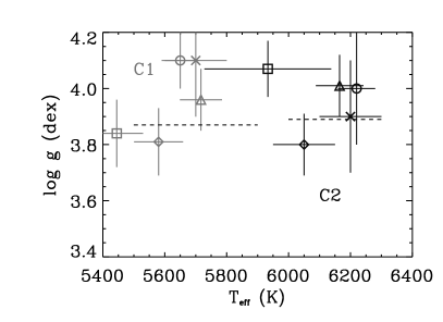
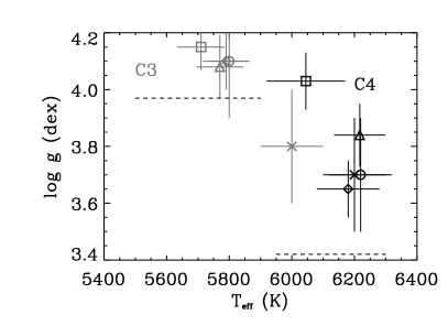
Figure 1: $T_{\rm eff}$ and $\log g$ derived from five spectroscopic analyses. Each symbol represents the results from one analysis method: $\triangle$=SOU, $\square$=ROTFIT, $\diamond$=VWA, $\circ$=BIA, $\times$=NIEM. The dashed lines show the $\langle\log g_{\rm MR}\rangle$ values derived from the seismic data alone (see Sect. 4.1).

2.3 Photometrically derived atmospheric parameters

Ground-based SLOAN-$griz$ photometry is available for a large number of stars in the field of view. The Kepler Input Catalog (KIC) lists the magnitude in the wide Kepler band pass, $Kp$, as well as the $griz$ magnitudes and the stellar parameters ($T_{\rm eff}$, [Fe/H], $\log g$, radius $R$) derived using these data. However, the primary purpose of the KIC was to allow discrimination of dwarfs from other classes of stars to aid in the selection of planet-hosting candidates. It has become clear since the time series data became available that the KIC $T_{\rm eff}$ are not always accurate on a star-to-star basis (Molenda-Żakowicz et al., 2010a, b; Lehmann et al., 2011). $T_{\rm eff}$ were, therefore, re-calculated by Pinsonneault & An (2011) using SLOAN photometry and the YREC models (An et al., 2009; Demarque et al., 2008), and cross-checking the results using the infra-red flux method calibration based on 2MASS photometry (Casagrande et al., 2010). The $T_{\rm eff}$ and uncertainties are listed in Table 3 with the heading ’P/A’.

3 Seismic methods

The nearly uninterrupted short-cadence Kepler time series yield power spectra that exhibit some signatures of oscillations. Even from low S/N power spectra, the global seismic quantities $\langle\Delta\nu\rangle$ and $\nu_{\rm max}$  can easily be determined without having to measure individual frequencies. In preparation for the hundreds of stars in the Kepler data where these seismic parameters are readily available, several pipeline codes have been developed to use stellar models to infer the surface gravity $\log g$, mean density $\langle\rho\rangle$, radius $R$, mass $M$, and age $\tau$ of stars from the global seismic quantities supplemented with atmospheric parameters, such as $T_{\rm eff}$. In this analysis we used the following methods which are discussed below: CESAM2k/Mumbai (Mazumdar, 2005), Yale-Birmingham (Basu et al., 2010; Gai et al., 2011), RADIUS (Stello et al., 2009a; Metcalfe et al., 2010), SEEK (Quirion et al., 2010), and RadEx10 (Creevey in prep.). We used five different analysis methods in order to test the validity of our results, and to assess the performance of each code for producing reliable stellar parameters.

3.1 CESAM2k/Mumbai

The analysis using the CESAM2k stellar evolution code (Morel & Lebreton, 2008) is based on the comparison of both seismic and non-seismic observations ($q$={$\langle\Delta\nu\rangle$,$\nu_{\rm max}$, $T_{\rm eff}$,$\log g$,[Fe/H],$\langle\delta\nu_{02}\rangle$}) with those calculated from a grid of stellar evolution models. This version of CESAM2k uses the OPAL equation of state (Rogers & Nayfonov, 2002) and the OPAL opacities (Iglesias & Rogers, 1996) supplemented by the low temperature opacities of Alexander & Ferguson (1994). The solar mixture is given by Grevesse & Sauval (1998) and the NACRE nuclear reaction rates (Angulo, Arnould, & Rayet, 1999) are used. Convection is described by the standard mixing length theory (Böhm-Vitense, 1958). The models also include microscopic diffusion of helium and heavy elements, following the prescription of Proffitt & Michaud (1991) for masses $\leq 1.3$ M_⊙.

The grid of models used in this analysis spans the mass range of 0.80 M_⊙ to 1.70 M_⊙, in steps of 0.02 M_⊙. The initial metallicities of the models $Z_{\rm i}$ range from 0.005 to 0.030 in steps of 0.005, and for each value of $Z_{\rm i}$, five different combinations of ($X_{\rm i}$, $Y_{\rm i}$) are used, where $Y_{\rm i}$ is the initial helium fraction. Three mixing length parameters $\alpha=1.8,1.9,2.0$ are considered, and for stars with convective cores, we used convective overshoot to the extent of $\alpha_{\rm ov}\times H_{\rm P}$ ($H_{\rm P}$ = pressure scale height), with $\alpha_{\rm ov}$ = {$0.00,0.05,0.10,0.15,0.20,0.25$}. The stellar evolutionary tracks start from the zero age main sequence (ZAMS) and continue until $\log(T_{\rm eff})\approx 3.715$, which corresponds to on or near the red giant branch. For each model during the evolution, oscillation frequencies for low degree modes ($\ell=0,1,2,3$) are computed under the adiabatic approximation using the Aarhus pulsation package, ADIPLS (Christensen-Dalsgaard, 2008b).

For every star, the average large frequency separation was computed between the same frequency limits as used in the observed data for the corresponding star and run. The average was calculated by integrating the individual frequency separation as a function of frequency between the given limits and dividing by the frequency range. The frequency of maximum amplitude, $\nu_{\rm max}$, has been calculated using the scaling relation provided by Kjeldsen & Bedding (1995):

$$\nu_{\rm max}\simeq\frac{M/M_{\odot}}{(R/R_{\odot})^{2}\sqrt{T_{\rm eff}/5777\,{\rm K}}}3,050\mu{\rm Hz}$$ (1)

We constructed a reduced $\chi^{2}_{R}$ using the available data as follows:

$$\chi^{2}=\sum_{i=1}^{n_{\mathrm{par}}}\left(\frac{q_{i,\mathrm{obs}}-q_{i,\mathrm{mod}}}{\sigma_{i,\mathrm{obs}}}\right)^{2},$$ (2)

where the sum is over all the available constraints $q_{i}$, and $\chi^{2}_{R}$ takes into account the number of constraints. The subscripts “obs” and “mod” refer to the observed and model values, respectively. The quoted uncertainty in the $i$th observed data is denoted by $\sigma_{i,\mathrm{obs}}$. We sought the minima of $\chi^{2}_{R}$ to provide estimates of the stellar parameters. The quoted values of the parameters and their uncertainties are the midpoints and half the span of the ranges of parameters for which $\chi^{2}_{R}\leq 1$.

3.2 Yale-Birmingham

The Yale-Birmingham (Basu et al., 2010) code as described by Gai et al. (2011) is a grid-based method for determining a star’s mass, radius, and age. The grid of models was constructed using the Yale Rotation and Evolution Code (Demarque et al., 2008) in its non-rotating configuration. The input physics includes the OPAL equation of state tables, the OPAL temperature opacities supplemented with low temperature opacities from Ferguson, Alexander, & Allard (2005), and the NACRE nuclear reaction rates. All models include gravitational settling of helium and heavy elements using the formulation of Thoul, Bahcall, & Loeb (1994). We use the Eddington $T(\tau)$ relation (here $\tau$ means optical depth), and the adopted mixing length parameter is $\alpha=1.826$. An overshoot of $\alpha_{\rm ov}=0.2$ was assumed for models with convective cores. The grid consists of 820,000 individual models with masses ranging from 0.8 to 3.0 $M_{\odot}$ in steps of 0.2$M_{\odot}$. These models have [Fe/H] ranging from +0.6 to $-0.6$ dex in steps of 0.05 dex. We assume that [Fe/H] = 0 corresponds to the solar abundance ($Z_{\odot}/X_{\odot}=0.023$) as determined by Grevesse & Sauval (1998). The model value for $\nu_{\rm max}$ is calculated using Eq. (1), and $\langle\Delta\nu\rangle$  is determined using

$$\frac{\langle\Delta\nu\rangle}{\langle\Delta\nu\rangle_{\odot}}\simeq\sqrt{\frac{\rho}{\rho_{\odot}}}=\left(\frac{M}{M_{\odot}}\right)^{\frac{1}{2}}\left(\frac{R}{R_{\odot}}\right)^{-\frac{3}{2}}$$ (3)

where $\langle\Delta\nu\rangle_{\odot}$ = 134.9 $\mu$Hz (see Kjeldsen & Bedding 1995).

The Yale-Birmingham pipeline finds the maximum likelihood of a set of input parameters calculated with respect to the grid of models. The estimate of the parameter is obtained by taking an average of the points that have the highest likelihood. We average all points with likelihoods over 95% of the maximum value of the likelihood functions. For a given observational (central) input parameter set, the first key step in the method is generating 10,000 input parameter sets by adding different random realizations of Gaussian noise to the actual (central) observational input parameter set. The distribution of any parameter, say radius, is obtained from the central parameter set and the 10,000 perturbed parameter sets form the distribution function. The final estimate of the parameter is the median of the distribution. We used 1$\sigma$ limits from the median as a measure of the uncertainties.

The likelihood function is formally defined as

$$\mathcal{L}=\left(\prod^{n}_{i=1}\frac{1}{\sqrt{2\pi}\sigma_{i}}\right)\times\exp(-\chi^{2}/2),$$ (4)

where $\chi^{2}$ is given in Eq. 2, and $q$ $\equiv$ {$T_{\rm eff}$, [Fe/H], $\Delta\nu$, $\nu_{\rm max}$}. From the form of the likelihood function in Eq. 4 it is apparent that we can easily include more inputs, or drop some inputs depending on the availability of data.

3.3 RADIUS

The RADIUS pipeline (Stello et al., 2009a) is based on a large grid of ASTEC models (Christensen-Dalsgaard, 2008a) using the EFF equation of state (Eggleton et al., 1973). We used the opacity tables of Rogers & Iglesias (1995) and Kurucz (1991) (for $T<10^{4}$ K), with solar mixture of Grevesse & Noels (1993). Rotation, overshooting, and diffusion were not included. The grid was created with fixed values of the mixing-length parameter, $\alpha=1.8$, and the initial hydrogen abundance of $X_{\mathrm{i}}=0.7$. The resolution in $\log(Z/X)$ was 0.1 dex between $0.001<Z<0.055$, and the resolution in mass was $0.01\,M_{\odot}$ from 0.5 to $4.0\,M_{\odot}$. The evolution begun at the ZAMS and continued to the tip of the red giant branch. To convert between the model values of $Z$ and the observed [Fe/H], the pipeline used $Z_{\odot}=0.0188$ (Cox, 2000).

Each output parameter was determined by selecting the set of models that were within $\pm 3\sigma$ of the observed input data. We pinpointed a single best-fitting model using a $\chi^{2}$ formalism and the 1$\sigma$ uncertainty is estimated as 1/6 of the maximum range of the values of the selected models. The pipeline as described in detail by Stello et al. (2009a) had some slight modifications; for example, the large frequency separation was derived by scaling the solar value (see Eq. 3) instead of calculating it directly from the model frequencies.

3.4 SEEK

The SEEK procedure (Quirion et al., 2010) also makes use of a large grid of stellar models computed with the ASTEC code. This version of ASTEC uses the OPAL equation of state (Rogers, Swenson, & Iglesias, 1996) along with the OPAL plus Ferguson & Alexander opacity tables (Iglesias & Rogers, 1996; Alexander & Ferguson, 1994), the element to element ratios in the metallic mixture of Grevesse & Sauval (1998), and convection is treated with the mixing-length formulation of Böhm-Vitense (1958); the mixing length to pressure scale height ratio $\alpha$, characterizing the convective efficacy, is treated as a variable parameter in the SEEK fits. Neither diffusion nor overshooting is included. Oscillation frequencies for each model are calculated using the ADIPLS (Christensen-Dalsgaard, 2008b) code.

Two subgrids were created: the first subgrid comprises tracks with all combinations of $Z$ = [0.005, 0.01, 0.015, 0.02, 0.025, 0.03], $X_{\rm i}$ = [0.68, 0.70, 0.72, 0.74], and $\alpha$ = [0.8, 1.8, 2.8] while the second subset has $Z$ = [0.0075, 0.0125, 0.0175, 0.0225, 0.0275], $X_{\rm i}$ = [0.69, 0.71, 0.73], $\alpha$ = [1.3, 2.3]. Every subset is composed of 73 tracks spanning from 0.6 to 1.8 M_⊙ in steps of 0.02 M_⊙  and from 1.8 to 3.0 M_⊙ in steps of 0.1, and each track was evolved until just after the base of the giant branch or $\tau$ = 15$\times 10^{9}$ yrs. The metallicity combinations correspond to –0.61$\leq$ [Fe/H] $\leq$ 0.20.

SEEK compares an observed star with every model of the grid and makes a probabilistic assessment of the stellar parameters, with the help of Bayesian statistics. Its aim is to draw the contour of good solutions which is located around $\chi^{2}_{R}$. The priors used in that assessment are flat for the age, the metallicity, the initial helium ratio, and the mixing length parameter. The only non-flat prior is related to the initial mass function and makes use of the Chabrier (2001) IMF model, where $\xi(M)=0.019M^{n}$, with $n=-1.55$ for $M\leq 1.0M_{\odot}$ and $n=-2.70$ when $M>1.0M_{\odot}$. The details of the SEEK procedure, including the choice of priors, and an introduction to Bayesian statistics can be found in Quirion et al. (2010).

3.5 RadEx10

RadEx10 is a grid-based approach to determining the radius, mass, and age using some or all of the following as input {$\langle\Delta\nu\rangle$,$\nu_{\rm max}$,$T_{\rm eff}$,$\log g$,[Fe/H]}. It is based on the ASTEC code and uses the EFF equation of state of Eggleton et al. (1973) without Coulomb corrections, the OPAL opacities (Iglesias & Rogers, 1996) supplemented by Kurucz opacities at low temperatures, and solar mixture from Grevesse & Noels (1993). The nuclear reaction rates came from Bahcall & Pinsonneault (1992), convection is described by the mixing-length theory of Böhm-Vitense (1958), convective core overshooting is included with $\alpha_{\rm ov}$ set to 0.25, and diffusion effects are ignored.

The grid considers models with masses from 0.75 – 2.0 M_⊙ in steps of 0.05 M_⊙, ages from ZAMS to subgiant, $Z_{\rm i}$ spans 0.007 – 0.027 in steps of $\sim 0.003$, while $X_{\rm i}$ is set to 0.70: this corresponds to $Y_{\rm i}=0.263-0.283$. The mixing length parameter $\alpha=2.0$ is used, which was obtained by calibrating the solar data. To obtain the stellar properties of mass, radius, and age, we perturb the observations using a random Gaussian distribution, and compare the perturbed observations to the model observables to select an optimal model. The $R$, $M$, $\tau$, and their uncertainties are defined as the mean value of the fitted parameter from 10,000 realizations, with the standard deviations defining the 1$\sigma$ uncertainties.

4 Stellar properties

4.1 Constraining $\log g$ with seismic data

The quantity $\langle\Delta\nu\rangle$ is proportional to the mean density of the star (see eq. [3]) and $\nu_{\rm max}$ also scales with $R$ and $M$ (see eq. [1]). By making an assumption that these stars have roughly solar $T_{\rm eff}$ with a large uncertainty, the seismic data alone should give a robust estimate of $\log g$ by using the scaling relations for $\nu_{\rm max}$ and $\langle\Delta\nu\rangle$ and solving for $R$ and $M$. The first two data columns in Table 4 show $\log g$ and its uncertainty, denoted by the subscript ’$\nu$’, when we use the seismic data and a $T_{\rm eff}$ estimate of 6000 K $\pm$ 500.

The grid-based methods described in Sect. 3 also used $\langle\Delta\nu\rangle$ and $\nu_{\rm max}$ from Table 2 as the only input observational data to their codes to obtain a model asteroseismic value of $\log g$. In this case we restricted the model $T_{\rm eff}$ to less than 8000 K. Table 4 shows the mean value of $\log g$, $\langle\log g_{\rm MR}\rangle$, obtained by combining the results from the five methods. We indicate that these are model-determined values by the subscript ’MR’. As can be seen, there is very good agreement between the model-independent and model-dependent values of $\log g$.

Figure 2 shows the difference between the asteroseismic $\log g$ value returned by each method, $\log g_{i}$, and $\langle\log g_{\rm MR}\rangle$. From left to right on the x-axis we show the results from SEEK, RADIUS, RadEX10, Yale-Birmingham, and CESAM2k/Mumbai (note the abbreviated labelling on the x-axis). For each seismic method, we show the differences in $\log g$ from left to right for stars C1, C2, C3, C4, C5, and the Sun. For the CESAM2k/Mumbai method ‘CMum‘, we show results for C1, C2, and C3 only, and these are labelled accordingly to avoid confusion.

The fitted $\log g$ values for each star and each method differ by $\sim$0.05 dex, excluding C4, with the largest differences seen primarily between the RADIUS and Yale-Birmingham methods, but still matching within 2$\sigma$. For C4 SEEK and RadEx10 give the largest dispersions, this difference reaching 0.13 dex. However, C4 is a very evolved MS star ($\log g$$\sim$3.50 dex) and the results for RadEx10 are biased, since this grid concentrates mostly in the MS and just beyond. If we ignore the result for RadEx10, we find a maximum difference between the results of 0.07 dex. The differences of 0.05 and 0.07 dex are still in much better agreement than the spectroscopic methods.

We also see that the statistical errors given by each method vary between 0.01 – 0.05 dex. However, all of the results fall to within 2$\sigma$ of the mean value. Each reported uncertainty is not underestimated, but some grids take into account some other variables, e.g. different mixing-length parameters, that will increase the reported value. For example, the uncertainties reported by Yale-Birmingham and RADIUS are indeed correct, however, because their grids are based on different physics and sets of parameters, they obtain results that differ by more than 1$\sigma$. Gai et al. (2010) did a systematic study of the uncertainties in stellar parameters determined by grid-based methods, including the Yale-Birmingham grid. Their study included a detailed investigation of the errors in $\log g$, and they found typical statistical uncertainties of $\leavevmode\nobreak\ 0.014$ dex when $T_{\rm eff}$ is included, in agreement with those reported here. They also tested the systematic errors by using different grids and different parameters (e.g. a different mixing-length parameter) and found that for stars similar to those used in this paper i.e. with similar $\langle\Delta\nu\rangle$, the half-width at half-maximum of the distribution of systematic errors is around $3$% in $\log g$ (see their Fig. 19, panel b). For a $\log g$ value of around 3.8, this would imply $\sigma\leq 0.1$ dex, in agreement with the differences in $\log g$ reported above.

As another example, the CESAM2k/Mumbai method reports results that take into account different values of the convective core overshoot parameter in the models. The inclusion of more parameters/physics will yield a more conservative error.

While distinguishing between the statistical uncertainties and the systematic errors is not always clear, we can be confident that combining the results from different grids provides a reliable determination of $\log g$ while the dispersion among the results is representative of a typical systematic error found by using different sets of physics and parameters. In order to provide accurate results with a conservative error we adopt the results from SEEK, whose uncertainty is larger than the dispersion among the fitted results. In Table 4, last three columns, we give an estimate of the systematic error, $\sigma_{\rm sys}={\rm max}\{|\log g_{\rm SEEK}-\log g_{i}|\}$, and the $\log g$ values and uncertainties provided by SEEK.

Table 4: Surface gravity obtained from $\langle\Delta\nu\rangle$ and $\nu_{\rm max}$ using scaling relations and stellar models, denoted by subscripts ’$\nu$’ and ’MR’, respectively.

Star	$\log g$ν	$\sigma_{\nu}$	$\langle\log g_{\rm MR}\rangle^{a}$	$\sigma_{\rm sys}$	$\log g$${}_{\rm MR}^{b}$	$\sigma_{\rm stat}^{b}$
	(dex)	(dex)	(dex)	(dex)	(dex)
C1	3.88	0.02	3.88	0.05	3.87	0.07
C2	3.88	0.03	3.89	0.04	3.89	0.06
C3	3.95	0.03	3.98	0.05	3.97	0.06
C4	3.47	0.04	3.49c	0.13c	3.42	0.06
C5	3.78	0.04	3.82	0.05	3.80	0.07
Sun	…	…	4.42	0.02	4.43	0.02

${}^{a}\langle\log g_{\rm MR}\rangle$ is the mean value of $\log g$ provided by all of the model results.
^b$\log g$_MR and $\sigma_{\rm stat}$ are the SEEK values.
^c Discarding the value from RadEx10 yields $\langle\log g\rangle$ = 3.46 and $\sigma_{\rm sys}$ = 0.07 dex.

4.2 Radius and mass

The atmospheric parameters $T_{\rm eff}$ and [Fe/H] are needed to derive the radius and mass of the star. Using the $\log g$ values obtained in Sect. 4.1 we selected one set of spectroscopic constraints as the optimal atmospheric parameters, and to minimise the effect of the correlation of spectroscopically derived parameters. We chose the set whose $\log g$ values matched closest globally to the asteroseismically determined ones. By inspecting Tables 3 and 4 we found that the VWA method has the overall closest results in $\log g$. We therefore combined these spectroscopic data with $\langle\Delta\nu\rangle$ and $\nu_{\rm max}$ from Table 2 and used these as the observational input data for the seismic analysis. For C5 we used the photometric $T_{\rm eff}$.

In Fig. 3 we show the deviation of the fitted radius of each method $R_{i}$ from the mean value $\langle R\,\rangle$ in units of %, with the mean radius in units of R_⊙ given in Table 5. The representation of the results is the same as in Fig. 2 i.e. from left to right for each method, we show C1, C2, C3, C4, C5, and the Sun. Most of the results are in agreement with the mean value at a level of 1$\sigma$, and the uncertainties vary between approximately 1 and 4 % (see Sect. 4.1). To be consistent, we adopt the SEEK method as the reference one. This choice is also justified by the following reasons: i) SEEK covers the largest parameter space in terms of mass, age, metallicity, and mixing-length parameter, ii) it has also been tested with direct measurements of mass and radius of nearby stars, iii) and it determines a best model parameter for each property (e.g. luminosity, initial metal mass fraction, and uncertainties), which allows us to make further inferences as well as investigate the systematics. In addition, it does not use the scaling relations, which may introduce a systematic bias on the order of 1% in the stellar parameters e.g. Stello et al. (2009b). We used the results from the other pipelines as a test of the systematic errors.

Figure 2: Comparison of each seismic method’s asteroseismic values of $\log g$ to the mean value $\langle\log g_{\rm MR}\rangle$ of the four or five methods. Each method is abbreviated and labelled on the x-axis, and for each method the results are shown from left to right for C1, C2, C3, C4, C5, and the Sun. The CMum (CESAM2k/Mumbai) method shows results for C1, C2, and C3 only.

Figure 3: Comparison of each seismic method’s determination of $R$ with the mean value $\langle R\,\rangle$ using both spectroscopic and seismic constraints. See caption of Fig. 2 for details.

Table 5: Radius determination from the SEEK method (first half of table) and combining all methods (second half of table) using spectroscopic and asteroseismic data.

Star	$R$	$\sigma$	$\sigma$	$\langle R\,\rangle$	$\sigma_{\rm sys}$	$\sigma_{\rm sys}$	$\sigma_{\rm sys}/\sigma_{i}$
	(R⊙)	(R⊙)	(%)	(R⊙)	(R⊙)	(%)
C1	2.23	0.04	2	2.21	0.06	3	2.3
C2	2.11	0.05	2	2.19a	0.22a	11	2.4
C3	1.90	0.05	3	1.88	0.07	4	1.2
C4	3.81	0.20	5	3.95b	0.38	10	2.2
C5	2.44	0.14	6	2.47	0.12	5	1.0
Sun	0.99	0.03	3	1.00	0.01	1	1.0

^a discarding the RADIUS result yields a value of 2.15 R_⊙ $\pm$ 0.09.
^b discarding the value from RadEx10 yields $\langle R\,\rangle=4.0$.

In Table 5 we list the $R$ values found using SEEK, the uncertainties $\sigma$, the mean value of $R$ obtained by combining the results from all of the grids $\langle R\,\rangle$, $\sigma_{\rm sys}={\rm max}\{|R_{\rm SEEK}-R_{i}|\}$ given in units of R_⊙, and $\sigma_{\rm sys}$ normalised by $\sigma_{i}$ i.e. ${\rm max}\{|(R_{\rm SEEK}-R_{i})/\sigma_{i}|\}$. Using SEEK with its reference set of physics, we determine the radius of each star with a typical statistical precision of 3%. If we use the results from the other pipelines as a measure of the systematic error, then we report an accuracy in the radius of between 3 and 5% for C1, C3, C5, and the Sun. The RADIUS method reports a radius that differs by 11% from the radius of the SEEK method for C2, but this difference corresponds to only 2.4$\sigma$ from the fitted $R$. Without this value $\sigma_{\rm sys}$ reduces to 5%. However, we have no justification to remove this value or discard the possibility that this is closer to the correct value. We remove the RadEx10 value for C4, but this results in an insignificant change ($<1$%). The method responsible for the largest deviation from the SEEK results for C4 is the Yale-Birmingham method, although they agree just above their 1$\sigma$ level. In the final column of the table we show the maximum deviation of the fitted radius from the SEEK radius but in terms of the uncertainty given by each pipeline method $\sigma_{i}$. Here we see that all of the results are consistent with SEEK to 2.4$\sigma$.

Table 6 reports the values of the mass determined by SEEK, and the other seismic methods, using the same format as Table 5. The statistical uncertainties are of the order of 8%, and the systematic errors are typically 5-12%, with each grid-based method reporting the same fitted mass to within 2.4$\sigma$. The fitted mass is highly correlated with the fitted radius, and thus most of the same trends are found among each pipeline method for both radius and mass. A much larger uncertainty in mass is reported for C5, and this is due to the lack of a metallicity constraint.

Table 6: Mass determination from the SEEK method (first half of table) and combining all methods (second half of table) using spectroscopic and asteroseismic data.

Star	$M$	$\sigma$	$\sigma$	$\langle M\,\rangle$	$\sigma_{\rm sys}$	$\sigma_{\rm sys}$	$\sigma_{\rm sys}/\sigma_{i}$
	(M⊙)	(M⊙)	(%)	(M⊙)	(M⊙)	(%)
C1	1.37	0.11	8	1.35	0.09	7	2.0
C2	1.26	0.10	8	1.37a	0.43a	34	2.4
C3	1.25	0.13	11	1.23	0.06	5	1.0
C4	1.79	0.12	7	1.84b	0.09b	5	1.5b
C5	1.44	0.26	18	1.50	0.18	12	1.6
Sun	0.97	0.06	7	1.01	0.08	9	1.0

^a discarding the RADIUS result yields a value of 1.32 R_⊙ $\pm$ 0.14.
^b discarding the value from RadEx10.

4.3 $\log g$ and $\langle\rho\rangle$ using combined seismic and spectroscopic data

Combining $\langle\Delta\nu\rangle$ and $\nu_{\rm max}$ with the VWA spectroscopic values of $T_{\rm eff}$ and the photometric value for C5, we calculated model-independent values of $\log g$ just as explained in Sect. 4.1. We also calculated the mean density of the star using $\langle\Delta\nu\rangle$. Table 7 lists these properties, again denoted by ’$\nu$’ to indicate that they are obtained directly from the data. We also give the model-dependent values of $\log g$_MR and $\langle\Delta\nu\,\rangle_{\rm MR}$ as reported by SEEK.

Both the $\log g$ and $\langle\rho\rangle$ values are in good agreement when derived directly from the data and when using stellar models. For $\log g$ there is agreement to 1.5$\sigma$, and for $\langle\rho\rangle$ the agreement is within 2.5$\sigma$. These values represent a relative precision of 2% for $\langle\rho\rangle$, with the exception of C4. In this case, the model $\langle\rho\rangle$ provides a more precise value than when using the seismic data alone, because the inclusion of atmospheric data helps to narrow down the range of possible values, when the uncertainty in $\langle\Delta\nu\rangle$ is large. The calculated solar value of 1,400 kg m^-3 is in excellent agreement with the true solar value (1,408 kg m^-3).

Comparing $\log g$_ν from Tables 4 and 7 we find values that differ by at most 0.02 dex ($<1\sigma$). This implies that by making a reasonable assumption about $T_{\rm eff}$, $\log g$ can be well estimated using only $\langle\Delta\nu\rangle$ and $\nu_{\rm max}$, or $\nu_{\rm max}$ alone.

Again, inspecting $\log g$ from Tables 4 and 7, but this time using the SEEK model-dependent values (’$\log g$_MR’) we also find that, apart from C4, the derived $\log g$ values are consistent with and without the atmospheric constraints, but the uncertainties in the latter reduce by a factor of 2 – 3. For C4 there is a difference of 0.1 dex between the two values, a change of nearly 2$\sigma$. As noted before this discrepancy is due to the relatively larger uncertainty in $\langle\Delta\nu\rangle$ when no atmospheric constraints are available.

Comparing SEEK to the other pipeline results for $\log g$, we find $\sigma_{\rm sys}$ of 0.02, 0.05, 0.01, 0.04, 0.02, and 0.02 dex, respectively. For the Kepler stars, these differences are smaller than $\sigma_{\rm SEEK}$ except for C2. The agreement between the $\log g$ values from the five seismic methods supports the results that we present, and we can be confident that any of the pipeline results using both seismic and atmospheric parameters can determine $\log g$ with a minimal systematic bias, just as Gai et al. (2011) showed.

We also find that the VWA spectroscopic values of $\log g$ agree with the model-dependent ones to within 1$\sigma$ for C1 and C2, and within 1.5$\sigma$ for C3 and C4.

Table 7: Surface gravity and stellar mean density obtained from scaling relations (’$\nu$’) and stellar models (’MR’) using both seismic and atmospheric constraints.

Star	$\log g$ν	$\log g$MR	$\langle\rho\rangle_{\nu}$	$\langle\rho\rangle_{\rm MR}$
	(dex)	(dex)	(kg m-3)	(kg m-3)
C1	3.86 $\pm$ 0.03	3.88 $\pm$ 0.02	175 $\pm$ 2	174 $\pm$ 4
C2	3.88 $\pm$ 0.03	3.88 $\pm$ 0.02	185 $\pm$ 1	189 $\pm$ 2
C3	3.94 $\pm$ 0.03	3.97 $\pm$ 0.03	254 $\pm$ 1	257 $\pm$ 5
C4	3.47 $\pm$ 0.03	3.52 $\pm$ 0.04	39$\pm$ 16	46 $\pm$ 4
C5	3.79 $\pm$ 0.04	3.82 $\pm$ 0.03	135 $\pm$ 1	140 $\pm$ 2
Sun	…	4.43 $\pm$ 0.01	…	1400 $\pm$ 18

4.4 Age

Determining the ages of the stars is a more complicated task since the value of the fitted age depends on the fitted mass and the description of the model. Figure 4 shows the fitted mass versus fitted age for stars C1 and C3 using five and four seismic methods, respectively (the CESAM2k/Mumbai method did not fit these data for C3 and C4). For both stars a correlation between the two parameters can be seen; a lower fitted mass will be matched to a higher age and vice versa. However, the uncertainties from the SEEK method ($\sim 1$ Gyr for a mass of 1.37 M_⊙ and $\sim 2$ Gyr for a 1.25 M_⊙ star) do capture the expected correlation with mass.

It is known that one of the physical ingredients to the models that has a large effect on the age of the star is the convective core overshoot parameter (see Sect. 5.2 below) where fuel is replenished by mixing processes that in effect extends the lifetime of the star. The CESAM2k/Mumbai method includes several values for this parameter among its grid of models, and this method fits an age of 5.3 Gyr for C1 (the SEEK method fits 3.9 Gyr). However, the fitted mass of the star is also lower than the SEEK one, and if we consider the uncertainty arising from the correlation with the age, then 5.3 Gyr is not outside of the expected range. For C2 the fitted mass for CESAM2k/Mumbai is 1.20 M_⊙ (SEEK = 1.26 M_⊙), and the fitted age is 4.4 Gyr (SEEK = 3.7 $\pm$ 0.7 Gyr). The difference between the fitted ages is 1$\sigma$, again not showing any difference due to the adopted values of the convective core overshoot parameter.

The final value of the age depends on the adopted model (stellar properties and physical description), but what seems to emerge from these data is that all of the stars are approaching or have reached the end of the hydrogen burning phase. In Table 8 we summarise the stellar properties obtained by adopting $\langle\Delta\nu\rangle$ and $\nu_{\rm max}$ from Table 2, the VWA spectroscopic constraints from Table 8, and the photometric $T_{\rm eff}$ for C5, while using the SEEK method (left columns) and combining the results from four (C3, C4, C5, Sun) and five (C1, C2) grid-based methods (right columns). We see that the mean values of the combined seismic methods results in stellar properties consistent within 1.5$\sigma$ of the SEEK results.

Table 8: Stellar properties obtained using $\langle\Delta\nu\rangle$, $\nu_{\rm max}$, and the atmospheric constraints from VWA for C1 – C4 and P/A for C5, from SEEK (first half of table) and by combining the results from all of the pipelines (second half of table).

Star	$\log g$	$R$	$M$	$\tau$	$\langle\log g\rangle$	$\langle R\,\rangle$	$\langle M\,\rangle$
	(dex)	(R⊙)	(M⊙)	(Gyr)	(dex)	(R⊙)	(M⊙)
C1	3.88$\pm$ 0.02	2.23$\pm$ 0.04	1.37$\pm$ 0.11	3.9$\pm$  1.4	3.87	2.21	1.35
C2	3.88$\pm$ 0.02	2.11$\pm$ 0.05	1.26$\pm$ 0.10	3.7$\pm$  0.7	3.89	2.19	1.37
C3	3.97$\pm$ 0.03	1.90$\pm$ 0.05	1.25$\pm$ 0.13	4.5$\pm$  1.8	3.97	1.88	1.23
C4	3.52$\pm$ 0.04	3.81$\pm$ 0.19	1.79$\pm$ 0.12	1.1$\pm$  0.2	3.52	3.95	1.87
C5	3.82$\pm$ 0.03	2.44$\pm$ 0.14	1.44$\pm$ 0.26	2.6$\pm$  0.9	3.82	2.47	1.50
Sun	4.43$\pm$ 0.01	0.99$\pm$ 0.03	0.97$\pm$ 0.06	9.2$\pm$  3.8	4.43	0.99	0.97

Figure 4: Fitted age versus mass for stars C1 ($\diamond$) and C3 ($\square$)

4.5 Including $\langle\delta\nu_{02}\rangle$ in the seismic analysis

With the individual oscillation frequencies available, the value of $\langle\delta\nu_{02}\rangle$ can be easily calculated. This observable can be particularly useful for determining the stellar age because it is determined by the sound-speed gradient in the core of the star, and as hydrogen is burned, a positive sound-speed gradient builds up. Three of the pipeline codes presented here do not allow one to use this value because it relies on the calculation of oscillation frequencies for every model in the grid, unlike $\langle\Delta\nu\rangle$ which can be derived from a scaling relation (c.f. Eq.3). We included $\langle\delta\nu_{02}\rangle$ as an extra constraint in SEEK to study the possible changes in the values and uncertainties of the stellar properties.

In Table 9 we list $\log g$, $R$, $M$, $\tau$, and the uncertainties without (first line for each star) and with (second line for each star) $\langle\delta\nu_{02}\rangle$ as an observational constraint. The first line for each star shows the same values as those presented in Table 8, and we repeat it here to make the comparison easier for the reader. For C1 we obtained a more precise determination of the age. For C2 and C3, no improvements in the parameters were found. For C5, all of the parameter uncertainties reduce by a factor of three, and the values of the parameters change by 1$\sigma$. The usefulness of $\langle\delta\nu_{02}\rangle$ here can most probably be explained by the lack of a metallicity constraint on the models. For the Sun we also found that the age improved from an estimate of 9.2 Gyr to 4.9 Gyr, very close to the accepted value. This last result can be explained by the fact that the stellar ’observables’ change on a much slower scale than for a more evolved star and hence provide weaker constraints.

Table 9: Comparison between fitted stellar properties using SEEK without (top lines) and with (bottom lines) $\langle\delta\nu_{02}\rangle$ as a seismic constraint.

Star	$\log g$	$R$	$M$	$\tau$
	(dex)	(R⊙)	(M⊙)	(Gyr)
C1	3.88$\pm$ 0.02	2.23$\pm$ 0.04	1.37$\pm$ 0.11	3.9$\pm$  1.4
	3.87$\pm$ 0.02	2.22$\pm$ 0.05	1.34$\pm$ 0.11	4.5$\pm$  0.5
C2	3.88$\pm$ 0.02	2.11$\pm$ 0.05	1.26$\pm$ 0.10	3.7$\pm$  0.7
	3.88$\pm$ 0.02	2.11$\pm$ 0.05	1.25$\pm$ 0.10	3.7$\pm$  0.6
C3	3.97$\pm$ 0.03	1.90$\pm$ 0.05	1.25$\pm$ 0.13	4.5$\pm$  1.8
	3.97$\pm$ 0.02	1.90$\pm$ 0.06	1.23$\pm$ 0.11	5.0$\pm$  1.9
C5	3.82$\pm$ 0.03	2.44$\pm$ 0.14	1.44$\pm$ 0.26	2.6$\pm$  0.9
	3.85$\pm$ 0.01	2.56$\pm$ 0.05	1.71$\pm$ 0.09	1.6$\pm$  0.2
Sun	4.43$\pm$ 0.01	0.99$\pm$ 0.03	0.97$\pm$ 0.06	9.2$\pm$  3.8
	4.43$\pm$ 0.01	1.01$\pm$ 0.03	1.01$\pm$ 0.04	4.9$\pm$  0.5

5 Sources of systematic errors

5.1 Using different spectroscopic constraints

We adopted the VWA spectroscopic constraints because their $\log g$ values were in best agreement with the asteroseismic ones given in Table 4, and later confirmed in Sect. 4.3. However, the VWA parameters may not be the optimal ones, and so we should investigate possible systematic errors arising from using the other atmospheric parameters from Table 3. We repeated the analysis using $\langle\Delta\nu\rangle$ and $\nu_{\rm max}$ with each set of atmospheric constraints to derive radius and mass. In Table 10 we give the six sets of observational data for star C1, and we label these S1 – S6. We also give the fitted radius and mass with uncertainties for each of these sets using the SEEK method.

Inspecting sets S1 – S5 we see that the largest differences between the fitted properties is 0.05 R_⊙ and 0.12 M_⊙($\sim$1$\sigma$), using sets S1 and S2. These differences can be attributed to both the input $T_{\rm eff}$ and [Fe/H] each contributing about equal amounts. At the level of precision of the spectroscopic $\log g$, this value has very little or no role to play in determining the radius and the mass, due to the tight constraints from the seismic data.

The results using S6, however, change by more than 1$\sigma$. This is clearly due to lacking metallicity constraints, and because C1 is considerably more metal-rich than the Sun. If the star had solar metallicity, the results would be comparable between each set. For example, for C3 which has solar metallicity we find a comparable radius using the photometric data (1.89 R_⊙) and the spectroscopic data (1.85 – 1.93 R_⊙). For C2 which has sub-solar metallicity we find the opposite trend to C1; the fitted radius is 2.18 R_⊙ without a metallicity constraint, while adopting the lower metallicity values yields smaller radii of 2.11 and 2.13 R_⊙. This same trend is found using the results from the other pipelines.

While the absence of a metallicity constraint in general increases the uncertainties e.g. from 0.05 to 0.11 R_⊙ for C1, with similar values found for C2 and C3, its absence will also bias the final fitted value of radius and hence mass, although still within its given uncertainty. For C4 the fitted radius varies by about 2% correlating directly with the input $T_{\rm eff}$ but the statistical uncertainty is 4 – 5%. In this case the absence of a metallicity measurement is unimportant, due to the error in $\langle\Delta\nu\rangle$ being a factor of 10 larger than for the other stars.

Table 10: Input spectroscopic observations (analysed along with the seismic data) for star C1 and the SEEK determination of mass and radius.

Set #	$T_{\rm eff}$	$\log g$	[Fe/H]	$R$	$\sigma_{\rm R}$	$M$	$\sigma_{\rm M}$
	(K)	(dex)	(dex)	(R⊙)		(M⊙)
S1	5717	3.96	+0.35	2.25	0.03	1.45	0.10
S2	5445	3.84	+0.13	2.20	0.05	1.33	0.10
S3	5580	3.81	+0.19	2.23	0.04	1.37	0.11
S4	5650	4.10	+0.36	2.25	0.04	1.44	0.10
S5	5700	4.10	+0.13	2.23	0.06	1.39	0.13
S6	5660	…	…	2.13	0.11	1.21	0.20

5.2 Different descriptions of the input physics

We reported the fitted properties (mass, radius, and age) and uncertainties for stars C1 – C5 in Table 8 using the reference method SEEK and the mean values obtained by combining the results from the four or five pipelines. We analysed the data using five grid-based seismic methods to test for the reliability of the results. Because the five methods are based on different sets of physics and input parameters, we can consider the scatter of the results from these pipelines as indicative of the systematic error that we can expect. Testing all of the possible sources of systematic errors in the most correct manner would imply generating numerous new grids with every combination of physics, stellar evolution codes, and parameters, and using the same analysis method that SEEK uses. While this is beyond the scope of this paper, and beyond the idea behind using grid-based methods, we can, however, investigate systematics by varying a few of the most important physical ingredients of the models, for example, the convective core overshoot parameter, and the inclusion/exclusion of diffusion. We keep in mind that the SEEK method covers almost the full range of possible mass, age, initial metal fraction, and mixing-length parameter for these stars, and the other pipelines use different combinations of EOS, opacities, nuclear reaction rates, and diffusion of elements (for some codes), and these should cover most of the systematics that one would expect to find.

We begun with a stellar model which is described by one set of stellar parameters P. SEEK provides central parameters defined by their distribution in the $\chi^{2}$ plane, so we used the SEEK parameters as a starting point to determine a single best-fitting model using the Levenberg-Marquardt minimisation algorithm, and the same input physics as SEEK. Because we have only five observations ($T_{\rm eff}$, $\log g$, [Fe/H], $\langle\Delta\nu\rangle$, $\nu_{\rm max}$) and in principle five fitting parameters ($M$, $\tau$, $Z_{\rm i}$, $X_{\rm i}$ or $Y_{\rm i}$, $\alpha$), we decided to fix the initial hydrogen mass fraction, which in effect allows $Y_{\rm i}$ to vary slightly, such that $Y_{\rm i}$ has near solar value, $Y_{i}=0.273-0.278$ (Serenelli & Basu, 2010). Table 11 lists the values of the best fitted parameters using the original input physics in SEEK and then for cases 1a – 1d and 2a – 2d, which are described below.

Once we have found P we change the physical description of the model by including convective core overshoot and setting its parameter to $\alpha_{\rm ov}=0.25$, and we search again for a new set of parameters that describe the observations best. We do this in various ways using the same minimisation algorithm. The first time we fit the same four parameters (case 1a), the second time we fit $\tau$, $Z_{\rm i}$ and $\alpha$ (case 1b), then we fit $M$, $Z_{\rm i}$ and $\alpha$ (case 1c), and finally we fit the parameters $M$ and $\alpha$ only (case 1d). If we fit both the mass and age together (case 1a), then we will determine a good model, but it is not possible to test if the new fitted mass and age are due to the ’correlation’ term between the parameters, or due to the new description of the model. For this reason we fix the mass and search for a set of parameters including the age that adequately fit the observations (case 1b) and vice versa (case 1c). This yields an estimate of the systematic error on the age/mass parameter for a fixed mass/age. We also include case (case 1d) to eliminate the $M$–$Y_{\rm i}$ correlation e.g. Metcalfe et al. (2009); Ozel et al. (2011). We repeat the same exercise while also including He diffusion as described by Michaud & Proffit (1993). These cases are denoted by 2a – 2d.

Table 11: The best-fitting parameters for star C1 found by using a minimisation algorithm with SEEK physics with some changes in the model.

Description	$M$	$R$	$\tau$	$Y_{\rm i}$	$Z_{\rm i}$	$\alpha$	$\chi^{2}_{R}$
	(M⊙)	(R⊙)	(Gyr)
	1.359	2.253	3.93	0.2706	0.0294	1.21	1.26
(1a) $\alpha_{\rm ov}=0.25$	1.386	2.275	3.81	0.2745	0.0255	1.33	1.73
(1b) $\alpha_{\rm ov}=0.25$	…	2.248	3.70	0.2774	0.0226	1.28	1.89
(1c) $\alpha_{\rm ov}=0.25$	1.386	2.264	…	0.2739	0.0261	1.39	1.49
(1d) $\alpha_{\rm ov}=0.25$	1.417	2.290	…	…	…	1.35	1.18
(2a) $\alpha_{\rm ov}=0.25$, He diff	1.379	2.265	3.74	0.2746	0.0254	1.30	1.75
(2b) $\alpha_{\rm ov}=0.25$, He diff	…	2.250	3.55	0.2763	0.0237	1.18	0.98
(2c) $\alpha_{\rm ov}=0.25$, He diff	1.379	2.271	…	0.2745	0.0255	1.40	1.22
(2d) $\alpha_{\rm ov}=0.25$, He diff	1.429	2.295	…	…	…	1.53	0.80

Inspecting Table 11, we find a maximum difference of 5% in mass and 1.8% in radius (case 2d), while the largest difference in the fitted age is found for case (2b) resulting in a 10% difference from the original fitted value. These systematic errors are much smaller than the uncertainties given by SEEK in Table 8. While we do not claim that these values are typical values for all combinations of physical descriptions in the models, these results indicate that the uncertainties are realistic. We may find larger differences using the more evolved stars, but the uncertainties for these stars are also generally larger.

6 Comparison of five grid-based approaches

Using the five Kepler stars and the Sun as test cases for grid-based analyses we have shown the following:

6.1 Surface gravity

If the seismic data alone are used to determine $\log g$ using stellar models, then we can expect to find systematic differences between the pipelines due to the different combinations of input physics. The difference between all of the results is at most 0.07 dex, which still provides a very strong constraint on $\log g$. Combining the results from all of the pipelines yields $\log g$ values in better agreement with those calculated directly from the seismic data (without models) when we make a modest assumption about $T_{\rm eff}$. When both atmospheric and seismic constraints are available, all of the pipelines yield consistent results for $\log g$, fitting to within at most 2$\sigma$ (or 0.05 dex) of either the SEEK result, the mean value from all the pipelines, or the model-independent value.

6.2 Radius and mass

The determination of mass, $M$, depends mostly on the value of the fitted radius, $R$, because the seismic data constrains the $M-R$ correlation. For this reason, similar trends are found for both $R$ and $M$. The systematic error ($\sigma_{\rm sys}$), defined here as the maximum difference in fitted values between SEEK and the other pipelines, was found to agree within $\sim$2$\sigma$. We also found that in general for the radius $\sigma_{\rm sys}$ increases with the evolutionary state of the star, i.e. 2% for the Sun which is mid-MS, and 10% for the most evolved star in this study (C4).

We adopted SEEK as the reference method, which has been validated with independent measurements of nearby stars, and we find that for each star, the mean parameter value obtained by combining the results from all of the pipelines agrees to within 1$\sigma$ of the SEEK results, e.g. $R_{\rm SEEK}-\langle R\,\rangle<1\sigma$ for all stars. This seems to imply that adopting an average value of the stellar parameters from several grid-based methods may be the optimal value to use. Nevertheless, all of the grids provide radius and mass values consistent within 2.4$\sigma$.

6.3 Age

In Fig. 4 we showed the fitted mass versus age for stars C1 and C3 using all of the methods for C1 and four methods for C3. While the returned value of the age depends upon the description of the physics and the mass of the star, in general we found the differences among the derived age is due to the mass-age correlation. Both the RADIUS and Yale-Birmingham pipelines provide the smallest uncertainties for C1. These are probably underestimated if one is to consider all possible sources of systematic errors.

When $\langle\delta\nu_{02}\rangle$ is available it is optimal to use the methods based on oscillation frequencies (SEEK, CESAM2k/Mumbai) in order to decrease the uncertainty in the age, especially for the less evolved MS stars e.g. for the Sun we find 9.2 $\pm$ 3.8 Gyr without $\langle\delta\nu_{02}\rangle$ and 4.9 $\pm$ 0.5 Gyr including it. However, the actual fitted value of age does not change very much for the more evolved MS stars analysed here.

7 Additional stellar properties from complementary data

7.1 Determination of distance

Table 12: Photometric data for C1 – C5 from the literature.

Star	$V^{a}$	$V^{b}$	$V^{c}$	E($B-V$)d
	(mag)	(mag)	(mag)	(mag)
C1	…	10.942	10.901	0.028
C2	10.871	10.840	10.959	0.056
C3	11.684	11.635	12.004	0.070
C4	11.982	11.885	12.160	0.075
C5	…	…	12.049	0.062

^a Urban et al. (1998) ^b Kharchenko (2001) ^c Droege et al. (2006) ^d KIC

The luminosities corresponding to the models from Table 8 yield values of the absolute bolometric magnitude $M_{\rm bol}$. To obtain the absolute $V$ magnitude $M_{V}$ we interpolate the tables from Flower (1996) for the values of $T_{\rm eff}$ given by VWA in Table 3 (and the photometric value for C5) to obtain the bolometric correction BC, and apply this correction to $M_{\rm bol}$. In Table 12 we list the apparent $V$ magnitudes from various sources. To account for reddening we use the standard extinction law A_V = 3.1$\times$E($B-V$), where 3.1 is a typical value (Savage & Mathis, 1979) and E($B-V$) are obtained from the KIC. We note that the adopted E($B-V$) should be used with caution (Molenda-Żakowicz et al., 2009). The distance modulus is calculated from $M_{V}$ and the de-reddened $V$, to give the asteroseismic distance $d$ in parsecs using $d=10^{0.2(V-M_{V})+1}$. In Table 13 we list the model $L$, $M_{V}$, the de-reddened $V$ magnitude adopting the values from Droege et al. (2006) $V_{\rm der}$, and the distance $d_{06}$, with the uncertainties arising from the luminosity uncertainty. The column with heading $d_{01}$ shows the distance using $V$ from Kharchenko (2001). We are able to determine distances to these stars with a precision of less than 10%. However, for C2 and C4 we find a discrepancy of 14% and 12% due to the different reported magnitudes.

We can also calculate the distance using one of the surface brightness relations from Kervella et al. (2004) (Table 5), if we know the radius. We used the relationship for $T_{\rm eff}$ and $V$; $\log\theta=3.0415(\log T_{\rm eff})^{2}-25.4696\log T_{\rm eff}+53.7010-0.2V_{\rm der}$, where $\theta$ is the angular diameter in milliarcseconds. Using the Droege et al. (2006) magnitudes, the fitted radii, and the observed $T_{\rm eff}$, we calculated the distance according to this relation $d_{\rm SB}$ (also given in Table 13), and these were found to agree with those using the distance modulus.

Table 13: Model luminosities $L$, absolute $V$ magnitudes $M_{V}$, de-reddened magnitudes $V_{\rm der}$, and asteroseismic distances from the standard distance modulus equation ($d_{06,01}$) and surface brightness relation $d_{\rm SB}$.

Star	$L$($\sigma_{\rm L}$)	$M_{V}$	$V_{\rm der}$	$d_{06}$	$d_{01}$	$d_{\rm SB}$
	(L⊙)	(mag)	(mag)	(pc)	(pc)	(pc)
C1	4.2 (1.1)	3.300	10.814	318${}^{+39}_{-45}$	324${}^{+40}_{-46}$	318$\pm$  20
C2	5.3 (1.1)	2.967	10.785	366${}^{+36}_{-40}$	347${}^{+34}_{-38}$	371$\pm$  24
C3	3.6 (1.2)	3.427	11.787	470${}^{+73}_{-86}$	396${}^{+61}_{-73}$	475$\pm$  31
C4	20.0 (1.1)	1.510	11.927	1212${}^{+33}_{-34}$	1068${}^{+29}_{-30}$	1231$\pm$  95
C5	7.8 (1.1)	2.526	11.857	735${}^{+50}_{-54}$	…	741$\pm$  61

7.2 Rotational period and inclination

The value of $v\sin i$ can be determined from the spectroscopic analysis (see Table 3). Combining this with $R$ allows us to constrain the stellar rotational period $P_{\rm ROT}$ – inclination $i$ relation. We use the $v\sin i$ values from ROTFIT to determine this relationship. With no observational constraints on $i$ for any star and having uncertainties in $v\sin i$ of the same order as its value for C3 (implying possibly $v\sin i$ $\sim 0$ kms^-1), the lower bound on $P_{\rm ROT}$ is unconstrained for all of the stars, while the upper bound is poorly restricted for C3. We can place an upper bound on $P_{\rm ROT}$ for C1, C2, and C4 of 384, 64, and 168 days, respectively.

Both Campante et al. (2011) and Mathur et al. (2011) analysed the low range of the frequency spectrum to look for signatures of a rotation period. They estimate $P_{\rm ROT}$ for C1, C2, and C3 of $\sim$ 36, 23, and 27 days, respectively, consistent with our results. Adopting these values as $P_{\rm ROT}$ constrains the stellar inclination angle $i=20^{\circ+18}_{\leavevmode\nobreak\ -15}$ for C1, $i=44^{\circ+46}_{\leavevmode\nobreak\ -23}$ for C2, and $i=25^{\circ+65}_{\leavevmode\nobreak\ -20}$ for C3.

7.3 Lithium content and age estimate

We noted that two of the investigated stars, namely C1 and C3, clearly display an Li i $\lambda$6707.8 Å  photospheric absorption line in the FIES spectra (Fig. 5), while for the remaining two stars the lithium line is not detectable. Lithium is burned at relatively low temperatures in stellar interiors ($\sim 2.5\,\times\,10^{6}$ K). As a consequence, it is progressively depleted from the stellar atmospheres of late-type stars when mixing mechanisms pull it deep into their convective layers. Therefore, its abundance can be used for estimating the stellar age, as shown by Sestito & Randich (2005) for stars belonging to 22 open clusters spanning the age range 0.005–8 Gyr.

We measured the equivalent width of the lithium line, correcting for the small contribution of the nearby Fe-I $\lambda$6707.4 Å  line as suggested by Soderblom et al. (1993), and found $W_{\rm Li}=102\pm 10$ mÅ  and $W_{\rm Li}=55\pm 10$ mÅ for C1 and C3, respectively. For C2 and C4, we estimated an upper limit for the lithium equivalent width $W_{\rm Li}<10$ mÅ as the product of the error of the normalised flux per spectral point and the integration width ($\simeq 1$ Å).

We derived a lithium abundance $\log n({\rm Li})=2.6\pm 0.1$ and $\log n({\rm Li})=2.4\pm 0.1$ for C1 and C3 by interpolation of the NLTE curves of growth tabulated by Pavlenko & Magazzù (1996), where by definition $\log n({\rm H})=12$. For C2 and C4, the lithium abundance is $\log n({\rm Li})<1.9$. The correlation of lithium abundance and age established by Sestito & Randich (2005, see their Fig. 7), suggests an age of 0.1 – 0.4 Gyr and 1 – 3 Gyr for C1 and C3, respectively, while their Table 3 suggests an age for C2 and C4 corresponding to the most evolved clusters in their study (M67 at 5 Gyr). The asteroseismic ages of 3 Gyr for C2 and 1 Gyr for C4 imply at least evolved MS stars for masses of 1.4 and 1.9 M_⊙, respectively.

New $W_{\rm Li}$ measurements for solar-like stars in galactic open clusters in the age range 1–8 Gyr, have shown that the low solar lithium abundance is not the standard for a star of that age and mass (Randich, 2010). In particular, Pasquini et al. (2008) found a spread of lithium abundance in stars of the solar-age cluster M 67, ranging from $\sim$0.4 to $\sim$2.0 dex. Randich (2010) also found that the average abundance for various clusters of similar age varies. For stars in the $T_{\rm eff}$ range 5750–6050 K, some evidence of bimodality in lithium depletion after 1 Gyr seems to emerge from these new data, with some clusters following the solar behaviour of abundance decay and other ones forming a plateau with $\log n({\rm Li})=2.2-2.4$. It is now unclear what the driving mechanism for depletion is, but it appears that some other parameter apart from mass and age is playing a role.

This could reconcile the lithium abundance $\log n({\rm Li})=2.4\pm 0.1$ of C3 with the higher age derived by asteroseismology. However, for C1, whose temperature is significantly lower (more lithium depletion), the lithium abundance of $\log n({\rm Li})=2.6\pm 0.1$ is not compatible with the age of 4 Gyr deduced by asteroseismology. We note that C1 is the most metal-rich star studied in this paper.

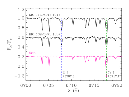
Figure 5: A region of the optical spectra which contains the Lithium $\lambda$6707.8 Å line. From top to bottom we show the spectra from C1, C3 and a high-resolution solar spectrum (Ganymede taken in 2007 with HARPS).

8 Summary and Conclusions

In this work we analysed the five solar-type stars KIC 11395018, KIC 10273246, KIC 10920273, KIC 10339342, and KIC 11234888, referred to as C1 – C5, respectively, based on more than eight months of short-cadence Kepler data. The global seismic quantities ($\langle\Delta\nu\rangle$ and $\nu_{\rm max}$) coupled with atmospheric parameters derived from photometry and spectra taken with the NOT telescope yield stellar properties with an average precision of 2% in mean density, $\sim$0.03 dex in surface gravity, 2–5% in radius, 7–11% in mass, and 35% in age (Table 14).

We used five grid-based approaches based on stellar models to estimate systematic errors, since the grids are all based on different physics and evolution codes. We found an agreement between all of the methods to within 2.4$\sigma$ for mass and radius, and these values were often comparable to the statistical uncertainties (see Tables 5 and 6). However, we also tested some specific sources of systematic errors arising from including convective core overshoot and settling of helium. We found that the fitted stellar parameters (radius, mass, and age) changed by an amount smaller than the statistical uncertainties reported in Table 14. These changes were also smaller than the dispersion among the results from the five grid-based methods, and we can therefore conclude that using several different methods provides an estimate of the systematic errors. However, since the value of the age is highly model-dependent, and we only tested two physical ingredients in the models, the systematic errors in the age could be larger. In Table 15 we summarise the estimates of the systematic errors $\sigma_{\rm sys}$ from various sources.

The spectroscopic data were analysed by five groups independently, each providing atmospheric parameters that varied by more than 200 K in $T_{\rm eff}$ and 0.2 dex for [Fe/H]. The differences obtained can be attributed to the quality of the spectroscopic data (low S/N and intermediate resolution). However, we found that the results are in general correlated (Fig. 3), indicating that with higher resolution and higher S/N data, the results should be in much better agreement. The different results obtained, however, also allowed us to study the influence of these atmospheric parameters for determining the radius and mass of the stars. We found that the fitted radius depends on both the adopted $T_{\rm eff}$ and [Fe/H], and the different values led to a discrepancy of about 2.5% in stellar radius and 8% in stellar mass. In the absence of an [Fe/H] measurement we found biased results in the fitted radius and mass for stars with non-solar metallicity (metal-rich C1 and metal-poor C2), and larger uncertainties. Higher-quality spectra should be obtained for these targets in the near future to match the exceedingly high quality of the Kepler data.

We investigated the role of including $\langle\delta\nu_{02}\rangle$ as an observational constraint with $\langle\Delta\nu\rangle$ and $\nu_{\rm max}$ (Sect. 4.5 and Table 9), and we found that $\langle\delta\nu_{02}\rangle$ is important primarily for the uncertainty in age for C1, C5, and the Sun. For C5 this is due to the absence of an [Fe/H] measurement. We suspect that its larger impact for the Sun, is because it is in the middle of its MS lifetime where the other atmospheric observables change relatively slowly with the age, thus providing weaker constraints.

Coupling photometric magnitudes with the model luminosities, we derived distances with a precision of less than 10%, and for C3 and C4, systematic errors of 14% and 12% respectively arise from the $V$ magnitudes reported by different authors. Later on in the mission, parallaxes may be obtained for the unsaturated stars. These independent determinations of distances should help to resolve the differences in the $V$ magnitudes and/or reddening.

By coupling the derived radius with the observed $v\sin i$, limits can be placed on the rotational period $P_{\rm ROT}$ of the stars. For C1, C2, and C4 we can impose an upper bound on $P_{\rm ROT}$ of 386, 67, and 177 days, respectively. Rotational period, inclination, and rotational velocity can all be determined in an independent manner by studying either the stellar spot distribution using the time series data, the frequency splittings in the power spectrum, or by studying the low frequency range of the power spectrum. Campante et al. (2011) and Mathur et al. (2011) study the low frequency range of the power spectra and estimate rotational periods of 36, 23, and 27 days for C1, C2, and C3, respectively. Adopting these as $P_{\rm ROT}$ constrains the stellar inclination angle $i=20^{\circ+18}_{\leavevmode\nobreak\ -15}$ for C1, $i=44^{\circ+46}_{\leavevmode\nobreak\ -23}$ for C2, and $i=25^{\circ+65}_{\leavevmode\nobreak\ -20}$ for C3.

The amount of lithium absorption in the atmospheric spectra can be used to estimate the age of the star. For the stars C2 and C4 no Li absorption is seen, indicating evolved MS stars, and this is confirmed by the seismic analysis. For C3, the Li abundance indicates an age that is inconsistent with the seismic value, but these could be reconciled, by considering new results which show a bimodal distribution of Li depletion (Randich, 2010). For the metal-rich star C1, however, the relatively high Li abundance indicates a non-evolved MS star, while the asteroseismic analysis suggests an incompatible value of $\sim 4$ Gyr.

Campante et al. (2011) and Mathur et al. (2011) analysed the time series and presented the oscillation frequencies for C1, C2, C3, and C5. Using the individual frequencies will yield more precise stellar properties, as well as studies of the stellar interior (Brandão et al. 2012, Doğan et al. 2012) as shown by Metcalfe et al. (2010). Up to now, such precise values have only been possible for members of detached eclipsing binaries, the Sun, and a few very bright stars. Thanks to the significant improvement in data quality from Kepler, this is about to change.

Table 14: Summary of stellar properties for KIC 11395018 (C1), KIC 10273246 (C2), KIC 10920273 (C3), KIC 10339342 (C4), and KIC 11234888 (C5), derived from atmospheric and mean seismic parameters, and stellar models.

	C1	C2	C3	C4	C5
a$\langle\rho\rangle$ν (kg m-3)	175$\pm$2	185$\pm$1	254$\pm$1	39$\pm$16	135$\pm$1
${}^{b}\langle\rho\rangle_{\rm MR}$ (kg m-3)	174$\pm$4	189$\pm$2	257$\pm$5	46$\pm$4	140$\pm$2
a$\log g$ν (dex)	3.86$\pm$0.03	3.88$\pm$0.03	3.94$\pm$0.03	3.47$\pm$0.03	3.79$\pm$0.04
b$\log g$MR (dex)	3.88$\pm$0.02	3.88$\pm$0.02	3.97$\pm$0.03	3.52$\pm$0.04	3.82$\pm$0.03
$R$ (R⊙)	2.23$\pm$0.04	2.11$\pm$0.05	1.90$\pm$0.05	3.81$\pm$0.19	2.44$\pm$0.14
$M$ (M⊙)	1.37$\pm$0.11	1.26$\pm$0.10	1.25$\pm$0.13	1.79$\pm$0.12	1.44$\pm$0.26
$\tau$ (Gyr)	3.9$\pm$1.4	3.7$\pm$0.7	4.5$\pm$1.8	1.1$\pm$0.2	2.6$\pm$0.9
c$\tau$⟨δν⟩ (Gyr)	4.5$\pm$0.5	3.7$\pm$0.6	5.0$\pm$1.9	…	1.6$\pm$0.2
$L$ (L⊙)	4.2$\pm$1.1	5.3$\pm$1.1	3.6$\pm$1.2	20.0$\pm$1.1	7.8$\pm$1.1
$T_{\rm eff}$model (K)	5547	6047	5789	6255	6180
$i$ (∘)	$20^{+18}_{-15}$	$44^{+46}_{-23}$	$25^{+65}_{-20}$	…	…
$P_{\rm ROTmax}$ (days)	384	64	…	168	…
${}^{d}P_{\rm ROTest}$ (days)	36 (6)	23	27	…	19–27 (5)
$d$ (pc)	318${}^{+39}_{-44}$	366${}^{+36}_{-40}$	470${}^{+72}_{-86}$	1212${}^{+33}_{-34}$	735${}^{+50}_{-54}$

^a,b Subscripts $\nu$ and MR indicate that the value was obtained directly from the data and from the models, respectively.
${}^{c}\tau_{\langle\delta\nu\rangle}$ is when $\langle\delta\nu_{02}\rangle$ is included as an observational constraint. In this case the uncertainties in $\log g$, $R$, and $M$ for C5 reduce by a factor of three.
${}^{d}P_{\rm ROTest}$ as reported by Campante et al. (2011) and Mathur et al. (2011), with uncertainties in parenthesis.

Table 15: Estimates of systematic errors in the stellar properties, given in CGS units for $g$, solar units for $R$ and $M$, and Gyr for age, with % values shown in parentheses.

	C1	C2	C3	C4	C5
$\sigma_{\log g,{\rm grid}}$	0.02	0.05	0.01	0.04	0.02
$\sigma_{R,{\rm grid}}$	0.06 (3)	0.22 (11)	0.07 (4)	0.38 (10)	0.12 (5)
$\sigma_{M,{\rm grid}}$	0.09 (7)	0.43 (34)	0.06 (5)	0.09 (5)	0.18 (12)
$\sigma_{\tau,{\rm grid}}$	1.4 (36)	1.7 (38)	1.8 (40)	0.2 (18)	0.4 (16)
$\sigma_{R,{\rm spec}}$	0.05 (2)	0.08 (4)	0.03 (2)	0.18 (5)	…
$\sigma_{M,{\rm spec}}$	0.13 (9)	0.16(13)	0.03 (2)	0.12 (7)	…
$\sigma_{R,{\rm phys}}$	0.06 (3)	…	…	…	…
$\sigma_{M,{\rm phys}}$	0.05 (4)	…	…	…	…
$\sigma_{\tau,{\rm phys}}$	0.35 (9)	…	…	…	…

The subscripts ’grid’, ’spec’, and ’phys’ mean estimates of systematic errors from using different grids/pipelines, different atmospheric constraints, and different descriptions of the physics in the models, respectively (see Sects. 4 and 5 for details).

Appendix A Oscillation frequencies

In Table 16 we list the published oscillation frequencies from Campante et al. (2011) and Mathur et al. (2011) for stars C1, C2, C3, and C5.

Table 16: Published frequencies given in $\mu$Hz for stars KIC 11395018 (C1), KIC 10273246 (C2), KIC 10920273 (C3), and KIC 11234888 (C5), as reported by Campante et al. (2011) and Mathur et al. (2011).

$l$	KIC 11395018	KIC 10273246	KIC 10920273	KIC 11234888
	C1	C2	C3	C5
0	686.66 $\pm$ 0.32	737.90 $\pm$ 0.30	826.66a $\pm$ 0.25	627.67 $\pm$ 0.19
0	732.37 $\pm$ 0.18	785.40 $\pm$ 0.20	882.77 $\pm$ 0.20	669.35 $\pm$ 0.16
0	779.54 $\pm$ 0.14	833.90 $\pm$ 0.20	939.58 $\pm$ 0.16	711.63 $\pm$ 0.15
0	827.55 $\pm$ 0.15	883.50 $\pm$ 0.20	997.14 $\pm$ 0.18	753.64 $\pm$ 0.20
0	875.40 $\pm$ 0.16	932.70 $\pm$ 0.50	1054.33 $\pm$ 0.30	794.56 $\pm$ 0.20
0	923.16 $\pm$ 0.19	981.10 $\pm$ 0.30	1111.51 $\pm$ 0.25	836.83 $\pm$ 0.21
0	971.05 $\pm$ 0.28	1030.70 $\pm$ 0.40	1170.77a $\pm$ 0.33	877.80a $\pm$ 0.22
0	…	1079.30 $\pm$ 0.20	1226.34a $\pm$ 0.33	…
1	667.05a $\pm$ 0.22	622.80 $\pm$ 0.20	794.65b $\pm$ 0.32	506.72 $\pm$  0.20
1	707.66 $\pm$ 0.19	661.90 $\pm$ 0.50	838.61b $\pm$ 0.25	563.30 $\pm$ 0.14
1	740.29b $\pm$ 0.17	695.75b $\pm$ 0.27	914.52 $\pm$ 0.16	594.83 $\pm$ 0.16
1	763.99 $\pm$ 0.18	724.70 $\pm$ 0.20	968.19 $\pm$ 0.13	686.34 $\pm$ 0.17
1	805.74 $\pm$ 0.13	764.30 $\pm$ 0.30	1023.58 $\pm$ 0.14	741.10 $\pm$ 0.18
1	851.37 $\pm$ 0.11	809.80 $\pm$ 0.20	1079.10 $\pm$ 0.31	815.43 $\pm$ 0.21
1	897.50 $\pm$ 0.15	857.30 $\pm$ 0.20	1135.36c $\pm$ 0.31	855.67 $\pm$ 0.21
1	940.50 $\pm$ 0.15	905.60 $\pm$ 0.30	…	…
1	997.91 $\pm$ 0.33	950.00 $\pm$ 0.30	…	…
1	…	1008.60 $\pm$ 0.40	…	…
1	…	1056.30 $\pm$ 0.20	…	…
1	…	1103.30 $\pm$ 0.40	…	…
2	631.19a $\pm$ 1.36	688.50 $\pm$ 0.70	822.39a $\pm$ 0.28	582.84a $\pm$ 0.21
2	680.88 $\pm$ 0.45	734.80 $\pm$ 0.60	873.10a,d $\pm$ 0.32	624.65 $\pm$ 0.18
2	727.78 $\pm$ 0.30	779.50 $\pm$ 0.40	934.49 $\pm$ 0.22	708.67 $\pm$ 0.19
2	774.92$\pm$ 0.16	830.30 $\pm$ 0.40	992.44 $\pm$ 0.13	751.84 $\pm$ 0.21
2	823.50 $\pm$ 0.16	880.60 $\pm$ 0.50	1049.36 $\pm$ 0.39	…
2	871.29 $\pm$ 0.21	927.50 $\pm$ 0.40	1106.76 $\pm$ 0.34	…
2	918.10 $\pm$ 0.28	977.60 $\pm$ 0.40	…	…
2	965.83 $\pm$ 0.23	1025.30 $\pm$ 1.30	…	…
2	1016.61a,f $\pm$ 0.73	1073.70 $\pm$ 0.20	…	…
2	…	1122.70a,d $\pm$ 0.40	…	…

The frequencies were fitted with 11, 10, 10, and 11 different methods, and a criteria was imposed to obtain a minimal frequency set representative of the results from most of the fitters.
^a Frequencies not among the minimal set.
^b $l=1$ mixed mode.
^c Mode close to the second harmonic of the inverse of the long-cadence period.
^d Possible $l=2$ mixed mode introduced a posteriori.
^e Uncertain identification.
^f Mode tagging changed a posteriori from $l=0$ to $l=2$.

Appendix B Atmospheric analysis methods

B.1 BIA

The MOOG code (version 2002; Sneden 1973) determines the iron abundance under the assumption of local thermodynamic equilibrium (LTE), using a grid of 1D model atmospheres by Kurucz (1993). The LTE iron abundance of C1 – C4 was derived from the equivalent widths of 55–68 Fe-I and 11 Fe-II lines in the 4830–6810 Å range, measured with a Gaussian fitting procedure in the IRAF task splot. For the analysis, we used the same list of lines as Biazzo et al. (2011) and we followed their prescriptions. In particular, $T_{\rm eff}$ and $\xi_{\rm t}$ were determined by requiring that the iron abundance be independent of the excitation potentials and the equivalent widths of Fe-I lines. The surface gravity was determined by requiring ionization equilibrium between Fe-I and Fe-II. The initial values for $T_{\rm eff}$, $\log g$  and $\xi_{\rm t}$ were chosen to be solar ($T_{\rm eff}$ = 5770 K, $\log g$ = 4.44 dex, and $\xi_{\rm t}$ = 1.1 km s^-1).

B.2 ROTFIT

The IDL code ROTFIT (Frasca et al., 2006) performs a simultaneous determination of $T_{\rm eff},\log g$, and [Fe/H] for a star, as well as its projected rotational velocity $v\sin i$, by comparing the observed spectrum with a library of spectra of reference stars (see, e.g., Katz et al. 1998; Soubiran et al. 1998). We estimated the stellar parameters and $v\sin i$ as the mean values for the 10 reference stars whose spectra, artificially broadened with $v\sin i$ in steps of 0.5 km s^-1, most closely resembled the target spectrum, and each is quantified by a $\chi^{2}$ measure. We adopted their standard deviation as a measure of the uncertainty. We applied the ROTFIT code to all echelle orders which cover the range 4300–6680 Å  in the observed spectrum. The adopted estimates for the stellar parameters come from a weighted mean of the values for all the individual orders, where more weight is assigned to the best fitted or higher S/N orders, and the “amount of information” contained in each spectral region expressed by the total spectral-line absorption. The standard error of the weighted mean was adopted as the uncertainty estimate for the final values of the stellar parameters. With the same code, we also performed an MK spectral classification for our targets.

B.3 NIEM

The NIEM analysis follows the methodology presented in Niemczura, Morel & Aerts (2009) and relies on an efficient spectral synthesis based on a least squares optimisation algorithm (see Takeda 1995). This method allows for the simultaneous determination of various parameters involved with stellar spectra and consists of the minimisation of the deviation between the theoretical flux distribution and the observed normalised one. The synthetic spectrum depends on the stellar parameters: effective temperature $T_{\rm eff}$, surface gravity $\log g$, microturbulence $\xi_{\rm t}$, rotational velocity $v\sin i$, radial velocity $v_{\rm R}$, and the relative abundances of the elements. The first three parameters are obtained before the determination of abundances of chemical elements and they are considered as input parameters. All the other above-mentioned parameters can be determined simultaneously because they produce detectable and different spectral signatures.

$T_{\rm eff}$, $\log g$, and $\xi_{\rm t}$ are adjusted by comparing the abundances determined from the unblended Fe-I and Fe-II lines. We require that the abundances measured from Fe-I and Fe-II yield the same result. The absorption lines of neutral iron depend only on $T_{\rm eff}$, $\xi_{\rm t}$, and iron abundance, and are practically independent of the surface gravity. On the other hand the lines of ionised iron are sensitive to the temperature, metallicity and most of all to gravity. First, we adjust $\xi_{\rm t}$ until there is no correlation between iron abundances and line intensity for the Fe-I lines. Second, $T_{\rm eff}$ is adjusted until there is no trend in the abundance versus excitation potential of the atomic level causing the Fe-I lines. Both $\xi_{\rm t}$ and $T_{\rm eff}$ are not independent, however the dependence on $\xi_{\rm t}$ is stronger, so we adjust this parameter first. The gravity is obtained by fitting Fe-II and Fe-I lines and requiring the same abundances from both neutral and ionised lines.

B.4 SOU

The SOU parameters were derived starting with the automatic measurement of equivalent widths of Fe-I and Fe-II lines with ARES (Sousa et al., 2007) and then imposing excitation and ionization equilibrium using a spectroscopic analysis in LTE with the help of the code MOOG (Sneden, 1973) and a GRID of Kurucz Atlas 9 plane-parallel model atmospheres (Kurucz, 1993). The Fe I and Fe II line list is composed of more than 300 lines that were individually tested in high resolution spectra to check its stability to an automatic measurement with ARES. The atomic data of the lines were obtained from the Vienna Atomic Line Database (Kupka et al., 1999) but the $\log gf$ were recomputed through an inverse analysis of the solar spectrum allowing in this way to perform a differential analysis relative to the Sun. A full description of the method can be found in Sousa et al. (2008). The errors on the SOU parameters are obtained by quadratically adding 60 K, 0.1 and 0.04 dex to the internal errors on $T_{\rm eff}$, $\log g$, and [Fe/H], respectively. These values were obtained considering the typical dispersion plotted in each comparison of parameters presented in Sousa et al. (2008). A more complete discussion about the errors derived for this spectroscopic method can be seen in Sousa et al. (2011).

B.5 VWA

The VWA software (Bruntt et al., 2010) relies on spectral synthesis of the region around individual Fe lines, but includes the contribution from weakly blending lines. The selection of lines was chosen from the degree of blending. These were then fitted with a synthetic spectrum. We adopted the MARCS model atmospheres (Gustafsson et al., 2008) and used the atomic line data from the Vienna Atomic Line Database (Kupka et al., 1999). Each line fit was inspected in great detail and bad fits discarded, resulting in between 100–150 Fe-I/Fe-II lines that were used in the parameter determination. The oscillators strengths $\log gf$ were corrected relative to the Sun as done in Bruntt et al. (2010). The values quoted in the Kepler Input Catalogue were used as initial guesses for the parameters of the atmosphere. The parameters were then refined through several iterations where each parameter was adjusted so that any correlations between the abundances of Fe-I and equivalent width (EW) and excitation potential (EP) were removed. Also, we required agreement between the Fe-I  and Fe-II abundances. Only lines with an ${\rm EW}\leq 90\,m$Å were used, since these lines are the most sensitive to changes in the fundamental parameters of the star.

To calculate the uncertainties of $T_{\rm eff}$, $\log g$, and $\xi_{\rm t}$ the model parameters were changed one at a time, until at least a 3$\sigma$ deviation was produced on the slope of the Fe-I-abundance vs. EP or EW, or between the Fe-I/Fe-II abundances. From these, the 1$\sigma$ error was calculated, giving the internal precision of the parameters calculated in VWA (Bruntt et al., 2008). The uncertainty on [Fe/H] was calculated as the standard error on the mean from Fe-I lines and adding quadratically the uncertainty from the model $T_{\rm eff}$, $\log g$, and $\xi_{\rm t}$.

To put further constraints on the $\log g$ value of the targets stars, we also used individual fits of the pressure-sensitive Mg ib lines and the Ca lines at $\lambda 6122$Å, $\lambda 6162$Å   and $\lambda 6439$Å. Each line was fitted with three different synthetic spectra, each with a different value for $\log g$. For each fit the $\chi^{2}$ was calculated and from this the best value of $\log g$ was determined. The method is described in greater detail in a paper by Bruntt et al. (2010). The final values for $\log g$ were taken as the weighted mean of the values found from matching the Fe-I/Fe-II abundances and from fitting the pressure-sensitive lines.

References

- Aerts et al. (2010) Aerts, C., Christensen-Dalsgaard, J., & Kurtz, D. W. 2010, Asteroseismology, Springer, 2010.
- An et al. (2009) An, D., et al. 2009, ApJ, 707, L64
- Angulo, Arnould, & Rayet (1999) Angulo, C., Arnould, M., Rayet, M., et al. 1999, Nucl. Phys. A., 656, 3
- Alexander & Ferguson (1994) Alexander, D. R., & Ferguson, J. W. 1994, ApJ, 437, 879
- Appourchaux et al. (2008) Appourchaux, T., et al. 2008, A&A, 488, 705
- Baglin (2003) Baglin, A. 2003, Advances in Space Research, 31, 345
- Bahcall & Pinsonneault (1992) Bahcall, J. N., & Pinsonneault, M. H. 1992, ApJ, 395, L119
- Ballot et al. (2006) Ballot, J., García, R. A., & Lambert, P. 2006, MNRAS, 369, 1281
- Basu et al. (2010) Basu, S., Chaplin, W. J., Elsworth, Y. 2010, ApJ, 710, 1596
- Bedding et al. (2010) Bedding, T. R., et al. 2010, ApJ, 713, L176
- Biazzo et al. (2011) Biazzo, K., Randich, S., & Palla, F. 2011, A&A, 525, A35
- Böhm-Vitense (1958) Böhm-Vitense, E. 1958, Z. Astrophys., 46, 108
- Borucki et al. (2010) Borucki, W. J., et al. 2010, Science, 327, 977
- Broomhall et al. (2009) Broomhall, A.-M., Chaplin, W. J., Davies, G. R., Elsworth, Y., Fletcher, S. T., Hale, S. J., Miller, B., & New, R. 2009, MNRAS, 396, L100
- Brown & Gilliland (1994) Brown, T. M., & Gilliland, R. L. 1994, ARA&A, 32, 37
- Bruntt et al. (2008) Bruntt, H., De Cat, P., & Aerts, C. 2008, A&A, 478, 487
- Bruntt et al. (2010) Bruntt, H., et al. 2010, MNRAS, 405, 1907
- Campante et al. (2010) Campante, T. L., Karoff, C., Chaplin, W. J., et al. 2010, MNRAS, 408, 542
- Campante et al. (2011) Campante, T. L., Handberg, R., Mathur, S., et al. 2011, A&A, 534, A6
- Casagrande et al. (2010) Casagrande, L., Ramírez, I., Meléndez, J., Bessell, M., & Asplund, M. 2010, A&A, 512, A54
- Castelli & Hubrig (2004) Castelli, F. & Hubrig, S. 2004, A&A, 425, 263
- Chabrier (2001) Chabrier, G. 2001, ApJ, 554, 1274
- Chaplin et al. (2011) Chaplin, W. J., Kjeldsen, H., Christensen-Dalsgaard, J., et al. 2011, Science 332, 213
- Christensen-Dalsgaard (2005) Christensen-Dalsgaard, J. 2005, Highlights of Astronomy, 13, 397
- Christensen-Dalsgaard (2007) Christensen-Dalsgaard, J. 2007, IAU Symposium, 239, 393
- Christensen-Dalsgaard (2008a) Christensen-Dalsgaard, J. 2008a, Ap&SS, 316, 113
- Christensen-Dalsgaard (2008b) Christensen-Dalsgaard, J. 2008b, Ap&SS, 316, 13
- Creevey & Bazot (2011) Creevey, O. L. & Bazot, M. 2011, JPhCS, 271, 012038
- Creevey et al. (2007) Creevey, O. L., Monteiro, M. J. P. F. G., Metcalfe, T. S., Brown, T. M., Jiménez-Reyes, S. J., & Belmonte, J. A. 2007, ApJ, 659, 616
- Cox (2000) Cox, A. N. 2000, Allen’s astrophysical quantities (Allen’s astrophysical quantities, 4th ed. Publisher: New York: AIP Press; Springer, 2000. Editedy by Arthur N. Cox. ISBN: 0387987460)
- Deheuvels & Michel (2010a) Deheuvels, S., & Michel, E. 2010, Ap&SS, 328, 259
- Deheuvels et al. (2010b) Deheuvels, S., et al. 2010, A&A, 515, A87
- Demarque et al. (2008) Demarque, P., Guenther, D. B., Li, L. H., Mazumdar, A. & Straka, C. W. 2008, Ap&SS, 316, 311
- Droege et al. (2006) Droege, T. F., Richmond, M. W., Sallman, M. P., & Creager, R. P. 2006, PASP, 118, 1666
- Eggleton et al. (1973) Eggleton, P. P., Faulkner, J., & Flannery, B. P. 1973, A&A, 23, 325
- Ferguson, Alexander, & Allard (2005) Ferguson, J. W., Alexander, D. R., Allard, F., et al. 2005, ApJ, 623, 585
- Flower (1996) Flower, P. J. 1996, ApJ, 469, 355
- Frasca et al. (2006) Frasca, A., Guillout, P., Marilli, E., et al. 2006, A&A, 454, 301
- Freeman & Bland-Hawthorn (2002) Freeman, K., & Bland-Hawthorn, J. 2002, ARA&A, 40, 487
- Gai et al. (2011) Gai, N., Basu, S., Chaplin, W. J., & Elsworth, Y. 2011, ApJ, 730, 63
- García et al. (2009) García, R. A., et al. 2009, A&A, 506, 41
- García et al. (2011) García, R. A., Hekker, S., Stello, S. et al. 2011, MNRAS, 414, L6-10
- Gilliland et al. (2010a) Gilliland, R. L., et al. 2010a, PASP, 122, 131
- Gilliland et al. (2010b) Gilliland, R. L., et al. 2010b, ApJL, 713, 160
- Grevesse & Noels (1993) Grevesse, N., & Noels, A. 1993, in Origin and Evolution of the Elements, ed. S. Kubono & T. Kajino (Cambridge: Cambridge Univ. Press), 14
- Grevesse & Sauval (1998) Grevesse, N., & Sauval, A. J. 1998, Space Science Reviews, 85, 161
- Gustafsson et al. (2008) Gustafsson, B., Edvardsson, B., Eriksson, K., Jørgensen, U. G., Nordlund, Å.,Plez, B. 2008, A&A, 486, 951
- Hekker et al. (2010) Hekker, S., Broomhall, A., Chaplin, W. J., et al. 2010, MNRAS, 402, 2049
- Hekker et al. (2010) Hekker, S., et al. 2010, ApJ, 713, L187
- Hekker et al. (2011) Hekker, S., et al. 2011, A&A, 525, A131
- Huber et al. (2009) Huber, D., Stello, D., Bedding, T. R., et al. 2009, CoAst, 160, 74
- Huber et al. (2010) Huber, D., et al. 2010, ApJ, 723, 1607
- Iglesias & Rogers (1996) Iglesias, C. A. & Rogers, F. J. 1996, ApJ, 464, 943
- Jenkins et al. (2010) Jenkins, J. M. et al. 2010, ApJL, 713, L87
- Kallinger et al. (2010) Kallinger, T., et al. 2010, A&A, 522, A1
- Karoff et al. (2010) Karoff C., Campante, T. L., & Chaplin, W. J. 2010, P19 of CD proceedings of “Seismological challenges for stellar structure”, AN, 331, Issue 9-10 (arXiv:1003.4167)
- Katz et al. (1998) Katz, D., Soubiran, C., Cayrel, R., Adda, M., & Cautain, R. 1998, A&A, 338, 151
- Kervella et al. (2004) Kervella, P., Thévenin, F., Di Folco, E., & Ségransan, D. 2004, A&A, 426, 297
- Kharchenko (2001) Kharchenko, N. V. 2001, Kinematika i Fizika Nebesnykh Tel, 17, 409
- Kjeldsen & Bedding (1995) Kjeldsen, H., & Bedding, T. R. 1995, A&A, 293, 87
- Kupka et al. (1999) Kupka, F., Piskunov, N., Ryabchikova, T. A., Stempels, H. C., Weiss, W. W. 1999, A&AS, 138, 119
- Kurucz (1991) Kurucz, R. L. 1991, in NATO ASIC Proc. 341, Stellar Atmospheres Beyond Classical Models, ed. L. Crivellari, I. Hubney, & D. G. Hummer (Dordrecht: Kluwer), 441
- Kurucz (1993) Kurucz, R. L. 1993, ATLAS9 Stellar Atmosphere Programs and 2 km s-1 grid, (Kurucz CD-ROM No. 13)
- Lehmann et al. (2011) Lehmann, H., Tkachenko, A., Semaan, T., Gutiérrez-Soto, J., Smalley, B., Briquet, M., Shulyak, D., Tsymbal, V., and De Cat, P. 2011, A&A, 526, 124
- Leibacher & Stein (1971) Leibacher, J. W., & Stein, R. F. 1971, ApJL, 7, 191
- Mathur et al. (2010a) Mathur, S., et al. 2010a, A&A, 518, A53
- Mathur et al. (2010b) Mathur, S., et al. 2010b, A&A, 511, A46
- Mathur et al. (2011) Mathur, S., Handberg, R., Campante, T.L. et al. 2011, ApJ, 733, 95
- Mazumdar (2005) Mazumdar, A. 2005, A&A, 441, 1079
- Metcalfe et al. (2009) Metcalfe, T. S., Creevey, O. L., & Christensen-Dalsgaard, J. 2009, ApJ, 699, 373
- Metcalfe et al. (2010) Metcalfe, T. S., et al. 2010, ApJ, 723, 1583
- de Meulenaer et al. (2010) de Meulenaer, P., Carrier, F., Miglio, A., Bedding, T. R., Campante, T. L., Eggenberger, P., Kjeldsen, H., & Montalbán, J. 2010, A&A, 523, A54
- Michaud & Proffit (1993) Michaud, G., & Proffitt, C. R. 1993, IAU Colloq. 137: Inside the Stars, 40, 246
- Miglio (2011) Miglio, A. 2011 (arXiv:1108.4555)
- Molenda-Żakowicz et al. (2009) Molenda-Żakowicz J., Jerzykiewicz M., and Frasca A. 2009, AcA 59, 213
- Molenda-Żakowicz et al. (2010a) Molenda-Żakowicz J. et al. 2010a, AN, 331, 981
- Molenda-Żakowicz et al. (2010b) Molenda-Żakowicz J., Jerzykiewicz, M., Frasca, A., Catanzaro, G., Kopacki, G., and Latham, D. W. 2010b, AN, 331, 9-10/P26 (arXiv:1005.0985v1)
- Morel & Lebreton (2008) Morel, P., & Lebreton, Y. 2008, Ap&SS, 316, 61
- Mosser et al. (2011) Mosser, B., et al. 2011, A&A, 532, 86
- Mosser et al. (2009) Mosser, B., et al. 2009, A&A, 506, 33
- Mosser & Appourchaux (2009) Mosser, B. & Appourchaux, T. 2009, A&A, 508, 877
- Niemczura & Połubek (2005) Niemczura, E., & Połubek, G. 2005, Memorie della Societa Astronomica Italiana Supplementi, 8, 210
- Niemczura, Morel & Aerts (2009) Niemczura, E., Morel, T., Aerts C., 2009, A&A, 506, 213
- Ozel et al. (2011) Ozel, N., Dupret, M. -A., & Baglin, A. 2011, A&A, 532, A82
- Pasquini et al. (2008) Pasquini, L., Biazzo, K., Bonifacio, P., Randich, S., & Bedin, L. R. 2008, A&A, 489, 677
- Pavlenko & Magazzù (1996) Pavlenko, Y. V., & Magazzù, A. 1996, A&A, 311, 961
- Proffitt & Michaud (1991) Proffitt, C. R., & Michaud, G. 1991, ApJ, 380, 238
- Quirion et al. (2010) Quirion, P.-O., Christensen-Dalsgaard, J., & Arentoft, T. 2010, ApJ, 725, 2176
- Randich (2010) Randich, S. 2010, in Light Elements in the Universe, Proceedings of the International Astronomical Union, IAU Symposium, Volume 268, p. 275
- Rogers & Iglesias (1995) Rogers, F. J., & Iglesias, C. A. 1995, in ASP Conf. Ser. 78, Astrophysical Applications of Powerful New Databases, ed. S. J. Adelman & W. L. Wiese (San Francisco, CA: ASP), 31
- Rogers, Swenson, & Iglesias (1996) Rogers, F. J., Swenson, F. J., & Iglesias, C. A. 1996, ApJ, 456, 902
- Rogers & Nayfonov (2002) Rogers, F. J. & Nayfonov, A. 2002, ApJ, 576, 1064
- Roxburgh (2009) Roxburgh, I. W. 2009, A&A, 506, 435
- Savage & Mathis (1979) Savage, B. D., & Mathis, J. S., 1979, ARA&A, 17, 73
- Sneden (1973) Sneden, C. 1973, ApJ, 184, 839
- Serenelli & Basu (2010) Serenelli, A. M., & Basu, S. 2010, ApJ, 719, 865
- Sestito & Randich (2005) Sestito, P., & Randich, S. 2005, A&A, 442, 615
- Soderblom et al. (1993) Soderblom, D. R., Jones, B. F., & Balachandran, S., et al. 1993, AJ, 106, 1059
- Soubiran et al. (1998) Soubiran, C., Katz, D., & Cayrel, R. 1998, A&AS, 133, 221
- Sousa et al. (2007) Sousa, S. G., Santos, N. C., Israelian, G., Mayor, M., & Monteiro, M. J. P. F. G. 2007, A&A, 469, 783
- Sousa et al. (2008) Sousa, S. G., et al. 2008, A&A, 487, 373
- Sousa et al. (2011) Sousa, S. G., et al. 2011, A&A, 526, A99
- Stello et al. (2009a) Stello, D., et al. 2009a, ApJ, 700, 1589
- Stello et al. (2009b) Stello, D., Chaplin, W. J., Basu, S., Elsworth, Y., & Bedding, T. R. 2009b, MNRAS, 400, 80
- Stello et al. (2010) Stello, D., et al. 2010, ApJ, 713, L182
- Suárez et al. (2010) Suárez, J. C., Goupil, M. J., Reese, D. R., Samadi, R., Lignières, F., Rieutord, M., & Lochard, J. 2010, ApJ, 721, 537
- Takeda (1995) Takeda, Y., 1995, PASJ, 47, 287
- Thoul, Bahcall, & Loeb (1994) Thoul, A. A., Bahcall, J. N. & Loeb, A. 1994, ApJ, 421, 828
- Ulrich (1970) Ulrich, R. K. 1970, ApJ, 162, 993
- Urban et al. (1998) Urban, S. E., Corbin, T. E., & Wycoff, G. L. 1998, VizieR Online Data Catalog, 1247, 0
- Van Grootel et al. (2010) Van Grootel, V., et al. 2010, ApJ, 718, L97
- Verner et al. (2011) Verner, G. A., Chaplin, W. J., Basu, S., et al. 2011, ApJ, 738, L28
- White et al. (2011) White, T. R., et al. 2011, ApJ 742, 3