Topological insulator ribbon: Surface states and dynamical response

Abstract

We study theoretically the distributions of charge and spin polarization of a topological insulator ribbon, with a realistic rectangular cross section. Due to constriction in two lateral directions, the surface states discretize into a series of subbands inside of the bulk band gap. The charge and spin distribution show interesting characters which are different from an ideal topological surface state. The effect of merging of four different surface states into the new one as an entity are analyzed. Optical conductivity and dynamical spin susceptibility of the ribbon are studied. Different from a single ideal surface, the optical response and dynamical spin susceptibility of a ribbon do not have a clear correspondence. The dynamical spin susceptibility could be used to identify the more adequate model for Bi₂Se₃.

I Introduction

The topological insulators are characterized by spin polarized helical boundary states protected by time reversal symmetry.kane05 ; bernevig06 ; fu07l ; fu07b ; roy09 In three dimensions, the Bi₂Se₃ material has attracted great attention because of its well defined Dirac cone like surface state dispersion.zhang09 ; xia09 Though perfect two-dimensional surface states account for the most essential properties of topological insulator, real samples also have lateral pairs of surfaces. For strong topological insulators, each surface carries an odd number of gapless topological surface modes.fu07l ; fu07b When the bulk material is constricted in two directions, we get a ribbon (or, nano-wire) of topological insulator.peng09 The Aharonov-Bohm effect of the Bi₂Se₃ ribbon showed interesting $\phi_{0}=h/e$ period oscillation and a conductance maximum at zero fluxpeng09 , which are in contradiction with both diffusive and ballistic transport and are explained theoretically in terms of impurity scattering effects.bardarson10 ; zhang10 More conventionally, the ribbon (nano-wire) of Bi₂Te₃, which is also a topological insulator and described by a model similar to that of Bi₂Se₃ zhang09 , is considered as a promising thermoelectrical material for applications.bejenari08 Former theoretical studies of topological insulator ribbon usually start from a cylindrical sample.lee09 ; bardarson10 ; zhang10 ; egger10 While an axi-symmetric configuration is more convenient for analytical analysis, a real topological ribbon usually has a rectangular cross-section.peng09 ; bejenari08 We thus study the charge and spin distributions of the surface modes of such a realistic topological insulator ribbon.

For a $\hat{z}\cdot(\mathbf{k}\times\bm{\sigma})$ (or equivalently, $\mathbf{k}\cdot\bm{\sigma}$) type of effective model for the surface states, the charge current operator is proportional to the spin operator. The optical conductivity for the surface states, which is defined in terms of the current-current correlation function, is correspondingly directly related to the dynamical spin susceptibility.raghu10 But for a topological insulator ribbon, in which two pairs of lateral surfaces are present, the relationship between the optical conductivity and the dynamical spin susceptibility would in general be more complicated. However, the results always depend uniquely on the characters of the model used, which also determine the properties of the surface states. The study of these responses may thus give some criteria to discriminate among available models for the topological insulator Bi₂Se₃.

In a previous work, two different models used in former works for Bi₂Se₃ were pointed out.hao11 Here, we propose that the more adequate model for the material could be identified by measuring the dynamical spin susceptibility of a Bi₂Se₃ ribbon. While optical conductivities are identical, the dynamical spin susceptibilities show clear qualitative differences between results obtained from the two models. The results are explained in terms of selection rule analysis based on direct numerical calculations. For optical conductivity, qualitatively different selection rules are in effect between transitions along the ribbon axis ($x$ direction in this work) and transitions along other directions.

II models and methods

Since we are interested mainly in the dynamical responses related to the topological surface states, it is reasonable to start from the continuum model for a topological insulator describing low energy states close to the $\Gamma$ point of the Brillouin zone (BZ).zhang09 ; fu09 ; fu10

Formerly, we recognized two different kinds of models that exist in the literature for bulk Bi₂X₃ (X is Se or Te) materials.fu09 ; wang10 ; fu10 ; li10nphys ; zhang09 ; liu10b1 ; liu10b2 ; lu10 ; shan10 ; li10 Close to the $\Gamma$ point, the two models could both be written compactly in terms of the Dirac matrices ashao11

$$H(\mathbf{k})=\epsilon_{0}(\mathbf{k})I_{4\times 4}+\sum\limits_{i=0}^{3}m_{i}(\mathbf{k})\Gamma_{i}.$$ (1)

Every unit cell contains two spin and two orbital degrees of freedom. The model is hence written in terms of 4 by 4 matrices. The two orbitals concentrate mainly on the top and bottom (looking along the $-z$ direction) Se layer of the various Bi₂Se₃ quintuple units, and are labeled as 1 and 2.wang10 ; fu10 The basis is taken as $\psi_{\mathbf{k}}$=[$c_{1\mathbf{k}\uparrow}$, $c_{2\mathbf{k}\uparrow}$, $c_{1\mathbf{k}\downarrow}$, $c_{2\mathbf{k}\downarrow}$]^T, for a certain wave vector in the three dimensional BZ. Since the first term proportional to the unit matrix is nonessential to topological properties of the system, it is ignored in the following analysis. The remaining model is particle hole symmetric. Close to the $\Gamma$ point, the four remaining coefficient functions are $m_{i=0,\cdots,3}(\mathbf{k})$=$\{m+\frac{3}{2}t(k_{x}^{2}+k_{y}^{2})+t_{z}k_{z}^{2},3tk_{x},3tk_{y},2t_{z}k_{z}\}$, in which $t>0$, $t_{z}>0$ and $m<0$ ($|m|$ is half of the bulk band gap).hao11 In terms of Pauli matrices $s_{i}$ ($i$=0, $\cdots$, 3) in the spin subspace and $\sigma_{i}$ ($i$=0, $\cdots$, 3) in the orbital subspace, the first three Dirac matrices are defined aszhang09 ; wang10 $\Gamma_{0}$=$s_{0}\otimes\sigma_{1}$, $\Gamma_{1}$=$s_{1}\otimes\sigma_{3}$, $\Gamma_{2}$=$s_{2}\otimes\sigma_{3}$. Two choices of the last Dirac matrix $\Gamma_{3}$ define the two different models in literature, which are: (I)$s_{0}\otimes\sigma_{2}$wang10 ; fu10 ; li10nphys and (II)$s_{3}\otimes\sigma_{3}$zhang09 ; liu10b1 ; liu10b2 ; lu10 ; shan10 ; li10 .

Though a full gap exists in the bulk, gapless modes reside on the surface. For surfaces directed along different directions, the surface states are described by different effective models. Take for example the surface states for a sample occupying the lower half $z$ space, the effective model for it was solved to behao11

$$H_{eff}(\mathbf{k})=3t(k_{x}s_{x}+k_{y}s_{y}),$$ (2)

for model I. The charge current matrix is thus $\mathbf{j}(\mathbf{k})=-e\mathbf{v}_{\mathbf{k}}=-e\nabla_{\mathbf{k}}H_{eff}(\mathbf{k})=-3et\mathbf{s}$. Where the Pauli matrices $s_{x}$ and $s_{y}$ are in terms of the two basis $(\eta_{1})_{\beta}$=$\delta_{\beta 1}$ and $(\eta_{2})_{\beta}$=$\delta_{\beta 3}$. $\delta_{\alpha\beta}$ is one for $\alpha$=$\beta$ and zero otherwise. While for model II, the effective model for the surface states of the same system ishao11

$$H_{eff}(\mathbf{k})=3t\hat{z}\cdot(\mathbf{k}\times\mathbf{s})=3t(k_{x}s_{y}-k_{y}s_{x}).$$ (3)

The corresponding charge current is $\mathbf{j}(\mathbf{k})$=$-3et\mathbf{s}\times\hat{z}$. The two bases are $\eta_{1}$=$\frac{1}{\sqrt{2}}[1,-i,0,0]^{T}$ and $\eta_{2}$=$\frac{1}{\sqrt{2}}[0,0,-i,1]^{T}$. For the surface states introduced above residing on the $xy$ surface, the two bases have definite spin characters for both model I and model II.

Now consider the surface states of a sample occupying the half space $y\leq 0$. Similar to surface states on the $z=0$ surface, the possible zero energy surface states on $y=0$ are obtained by solving a set of four coupled second order differential equations

$$H(k_{x}=0,k_{y}\rightarrow-i\partial_{y},k_{z}=0)\Psi(y)=E\Psi(y),$$ (4)

for $E=0$ together with the open boundary conditions $\Psi(y)|_{y=0}$=$\Psi(y)|_{y=-\infty}$=0.liu10b2 ; lu10 For model I, the basis for the surface states are obtained as $\eta_{1}$=$\frac{1}{\sqrt{2}}[1,0,0,1]^{T}$ and $\eta_{2}$=$\frac{1}{\sqrt{2}}[0,1,-1,0]^{T}$ by solving the above coupled differential equations. Now, both orbitals contribute to the surface states. The corresponding effective model turns out to be

$$H_{eff}(\mathbf{k})=-3tk_{x}\sigma_{x}+2t_{z}k_{z}\sigma_{y}.$$ (5)

While for model II, the surface states are described by an effective model as

$$H_{eff}(\mathbf{k})=-3tk_{x}\sigma_{x}+2t_{z}k_{z}\sigma_{z},$$ (6)

with the same basis set as for model I. The two basis states now do not have definite spin characters. On the other hand, the Dirac cone of the surface states becomes anisotropic, which is a manifestation of the uniaxial anisotropy of bulk states between the $xy$ plane and the $z$ direction. egger10

The above effective models for topological surface states describe infinite surfaces. A real sample is however finite in all three directions. For a ribbon geometry realized and studied recently, the sample could be considered as infinite along the direction of the ribbon axis (taken as $x$) while finite in the other two directions (taken as $y$ and $z$).peng09 Then, while $k_{x}$ could still be taken as a good quantum number, real space viewpoint should be adopted for $y$ and $z$ dependent quantities. For the sake of simplicity, we discretize the $y$ and $z$ coordinates into square lattices. The model is thus written as

$$H=\sum\limits_{n_{y},n_{z},k_{x}}\psi^{\dagger}_{n_{y}n_{z}}(k_{x})\sum\limits_{i=0}^{3}m^{{}^{\prime}}_{i}(k_{x})\Gamma_{i}\psi_{n_{y}n_{z}}(k_{x})$$

$$+\sum\limits_{n_{y},n_{z},k_{x}}\{\psi^{\dagger}_{n_{y}n_{z}}(k_{x})[-\Gamma_{0}-i\Gamma_{3}]t_{z}\psi_{n_{y},n_{z}+1}(k_{x})+H.c.\}$$

$$+\sum\limits_{n_{y},n_{z},k_{x}}\{\psi^{\dagger}_{n_{y}n_{z}}(k_{x})[-\Gamma_{0}-i\Gamma_{2}]\frac{3}{2}t\psi_{n_{y}+1,n_{z}}(k_{x})+H.c.\},$$ (7)

where $m^{{}^{\prime}}_{i=0,\cdots,3}(\mathbf{k})$=$\{m+3t+2t_{z}+\frac{3}{2}tk^{2}_{x},3tk_{x},0,0\}$. $n_{y}$ and $n_{z}$ label the unit cells along the $y$ and $z$ directions. The lattice constants along the three directions are taken as length units.

The paramagnetic current operators along three directions could be obtained by the continuity equations.hao09 They are written as

$$j^{P}_{x}=-e\sum\limits_{n_{y},n_{z},k_{x}}\psi^{\dagger}_{n_{y}n_{z}}(k_{x})(3tk_{x}\Gamma_{0}+3t\Gamma_{1})\psi_{n_{y}n_{z}}(k_{x}),$$ (8a)

$$j^{P}_{y}=e\sum\limits_{n_{y},n_{z},k_{x}}[\psi^{\dagger}_{n_{y}n_{z}}(k_{x})iD_{y}\psi_{n_{y}-1,n_{z}}(k_{x})+H.c.],$$ (8b)

$$j^{P}_{z}=e\sum\limits_{n_{y},n_{z},k_{x}}[\psi^{\dagger}_{n_{y}n_{z}}(k_{x})iD_{z}\psi_{n_{y},n_{z}-1}(k_{x})+H.c.],$$ (8c)

where $D_{y}$=$-\frac{3}{2}t(\Gamma_{0}-i\Gamma_{2})$ and $D_{z}$=$-t_{z}(\Gamma_{0}-i\Gamma_{3})$. In this work, we would focus on the zero temperature response behaviors of the system. The dynamical conductivity is obtained from the retarded current-current correlation functions by the Kubo’s formula.hao09 ; mahanbook Ignoring contribution from the diamagnetic current (which contributes to the zero frequency Drude weight), the expression is

$$\sigma_{\alpha\beta}(\omega)=\frac{i}{\omega}\Pi_{\alpha\beta}(\omega),$$ (9)

where the retarded current-current correlation function is defined as

$$\Pi_{\alpha\beta}(\omega)=-\frac{i}{V}\int_{-\infty}^{+\infty}dte^{i\omega t}\theta(t)\langle 0|[j^{P}_{\alpha}(t),j^{P}_{\beta}(0)]|0\rangle$$

$$=\frac{1}{V}\sum\limits_{n}[\frac{\langle 0|j^{P}_{\alpha}|n\rangle\langle n|j^{P}_{\beta}|0\rangle}{\omega+E_{0}-E_{n}+i\eta}-\frac{\langle 0|j^{P}_{\beta}|n\rangle\langle n|j^{P}_{\alpha}|0\rangle}{\omega+E_{n}-E_{0}+i\eta}]$$ (10)

$\{|n\rangle\}$ is a complete set of basis states, with $|0\rangle$ denoting the ground state. $E_{n}$ is energy of the state $|n\rangle$. $\eta$ is the positive infinitesimal and taken as a small positive number in realistic calculations.

The spin operator of the system is defined as $\mathbf{S}$ =$\frac{1}{2}\sum_{n_{y}n_{z}}\sum_{k_{x}}\psi^{\dagger}_{n_{y}n_{z}}(k_{x})\mathbf{s}\otimes\sigma_{0}\psi_{n_{y}n_{z}}(k_{x})$. The zero temperature dynamical spin susceptibility (for $\mathbf{q}=0$) is thus defined as

$$\chi_{ij}(\omega)=-\frac{i}{V}\int_{-\infty}^{+\infty}dte^{i\omega t}\theta(t)\langle 0|[S_{i}(t),S_{j}(0)]|0\rangle$$

$$=\frac{1}{V}\sum\limits_{n}[\frac{\langle 0|S_{i}|n\rangle\langle n|S_{j}|0\rangle}{\omega+E_{0}-E_{n}+i\eta}-\frac{\langle 0|S_{j}|n\rangle\langle n|S_{i}|0\rangle}{\omega+E_{n}-E_{0}+i\eta}].$$ (11)

III results and discussions

Without loss of generality, we consider a ribbon with $N_{y}$=$N_{z}$=20 and for $t$=$t_{z}$=0.5, $m$=-0.7. Fig. 1(a) is the dispersion of the ribbon. Within the bulk gap region ($|E|<-m$), sub-bands form with a finite minimal gap as a result of discretization of the topological surface states induced by lateral constriction. As shown in Fig. 1(a), the sub-bands are labeled symmetrically with respect to $E=0$ as $\{$$\pm 1$, $\pm 2$, $\ldots$$\}$, with positive (negative) sign denoting positive (negative) energy sub-bands and the larger numbering representing a larger distance to $E=0$. Every state is twofold degenerate due to combined time reversal symmetry and inversion symmetry of the material.

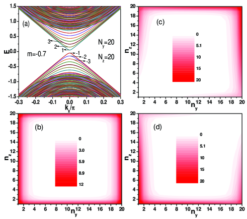
Figure 1: (a) Dispersion of a topological insulator ribbon with $N_{y}$=$N_{z}$=20. (b) Charge distribution (multiplied by $10^{3}$) of the surface modes $n$=3 for $k_{x}$=0, results for other $n$ (for $k_{x}$=0) within the bulk gap region are similar. (c) and (d) are the charge distribution (multiplied by $10^{3}$) of the two fold degenerate $n$=1 surface eigenmode for $k_{x}$=0.1$\pi$.

The charge and spin distributions of the topological surface states are essential to its physical properties. In the ribbon geometry, an interesting feature is related to the hybridization and redistribution of different surface states. We give the spin and charge distributions for several typical surface modes on the sub-bands within the bulk gap. As shown in Fig. 1(b) for the charge distribution of a typical surface mode for $k_{x}$=0, the charge is distributed centro-symmetrically close to the boundary of the ribbon’s cross-section. Around the cross-section, more charge is distributed close to the four corners which is easily understood from the smaller effective radius there compared to the flat part of the sample. As shown in Figs. 1(c) and 1(d), the charge distributions for the twofold degenerate modes of $n$=1 for $k_{x}$=0.1$\pi$ are asymmetric and centered around one corner of the ribbon, displaying clearly the effect of hybridization of two kinds of surface modes across the corner.

Figure 2: Spin distribution for a surface mode labeled as the first sub-band at $k_{x}$=0. The three components of the spin expectation value on every site are presented in (a), (b) and (c) (d, e and f) for model I (model II). The results in (a), (b) and (c) (in d, e and f) are multiplied by $10^{3}$ ($10^{4}$).

While the charge distributions are qualitatively identical along the $y$ and $z$ directions and are the same for the two different models, the spin distribution is more complicated. For a state residing on an infinite $xy$ surface, the spin only has in-plane component. While for states on an infinite $xz$ surface, the basis of the surface states indicate that the spin has both in plane and out of plane components. In the present ribbon geometry, the surface modes resulting from hybridization of the two types of surface modes would be different from an ideal surface. Fig. 2 shows distributions of the three spin components for a typical surface mode, which is one of the two degenerate modes for $n$=1 and $k_{x}$=0. Figs. 2(a, b, c) are for model I. A peculiar feature is that the expectation value of the $y$ spin component is everywhere zero. However, spin distributions of the corresponding surface state for model II shown in Figs. 2(d, e, f) have all the three spin components nonzero along the edge of the cross-section.

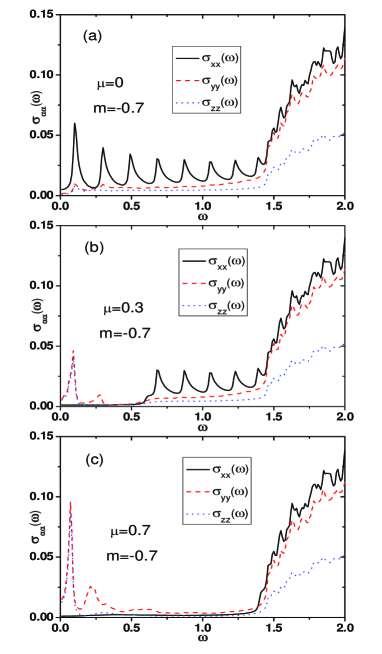
Figure 3: Longitudinal dynamic conductivity (optical conductivity) along $x$, $y$ and $z$ directions for three typical chemical potentials (a) $\mu=0$, (b) $\mu=0.3$, and (c) $\mu=0.7$. Results for the two models are identical. $2|m|=1.4$ is the bulk band gap. $\eta$=0.01.

Having the above charge and spin distributions of the surface sub-bands in mind, it is natural to expect that the charge response of the two models would be similar, but the spin responses would possibly show very different behaviors. Fig. 3 shows the optical conductivity (in unit of $e^{2}/\hbar$) of a ribbon with $N_{z}$=20 and $N_{y}$=20. The same results are found for the two models. The optical conductivity is defined as real part of the longitudinal dynamical conductivity and is related to optical absorption. One interesting feature is the low energy peaks of optical absorptions related to optical transitions between the surface sub-bands inside of the bulk band gap for $\omega<2|m|=1.4$.laforge10 When the chemical potential lies at the charge neutral point, only the $x$ component of the optical conductivity is significant. The $y$ and $z$ components of the optical conductivity are smaller and nearly featureless. When the chemical potential is shifted away from the Dirac point by $\Delta$, the low frequency part below 2$|\Delta|$ for $\sigma_{xx}$ is depleted while the higher frequency part remains unchanged. In contrast, some low frequency ($\omega$$\ll$$2|m|$) peaks emerges for $\sigma_{yy}$ and $\sigma_{zz}$. This reflects a difference in the selection rules of optical transitions along the three directions. Since $k_{x}$ is still a good quantum number, only vertical optical transitions between states with the same $k_{x}$ are allowed along all three directions, as could be seen from the current operators defined in Eq. (8).

Differences between $\sigma_{xx}$ and optical conductivities along the other two directions arise from selection rules with respect to $n$ in the optical transitions. Numerically, only transitions between pairs of sub-bands labeled by $n$ and $-n$ are allowed for optical transitions along the $x$ direction. While for optical transitions along $y$ and $z$, the transitions involving sub-band $n$ is largest with respect to $n\pm 1$. So, while for $\sigma_{xx}$ a series of peaks below 2$|m|$ are expected corresponding to transitions between $n$ and $-n$ sub-bands, $\sigma_{yy}$ and $\sigma_{zz}$ only have low frequency peaks corresponding to transitions between adjacent sub-bands. For nonzero $\Delta$, the low frequency ($\omega\leq 2|\Delta|$) optical transitions contributing to $\sigma_{xx}$ are strictly forbidden since the involved sub-band pairs are all occupied. Thus the corresponding low frequency part of $\sigma_{xx}$ is depleted. But for $\sigma_{yy}$ and $\sigma_{zz}$, the number of states that could contribute to low frequency optical absorptions continuously increases, resulting in a monotonic enhancement of the low frequency ($\omega\leq 2|\Delta|$) peaks with increasing $|\Delta|$. This nicely explains the evolution of the low frequency optical conductivities in Fig. 3.

We now proceed to calculate the dynamical spin susceptibilities. In accordance with the optical conductivity, we focus on the imaginary part of the dynamical spin susceptibilities. Only the longitudinal components would be analyzed here. For an ideal $xy$ surface, the optical conductivity is identical to the dynamical spin susceptibility. In the presence of $xz$ surface, another correspondence between optical conductivity and spin susceptibility specific to the $xz$ surface states mixes in. In Fig. 4 we show the imaginary parts of the longitudinal dynamical spin susceptibilities normalized by the frequency. In agreement with expectation based on the different spin distributions of the surface sub-bands, the dynamical spin responses for the two different models show qualitatively different behaviors and thus could be used as a means to tell the right model for Bi₂Se₃.

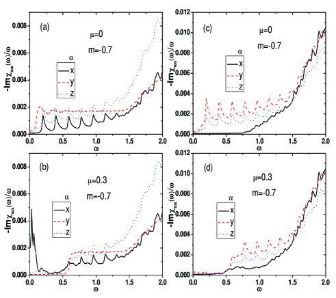
Figure 4: Dynamic spin susceptibility, the imaginary part normalized by the frequency. (a) $\mu=0$ for model I, (b) $\mu=0.3$ for model I, (c) $\mu=0$ for model II, (d) $\mu=0.3$ for model II. $2|m|=1.4$ is the bulk band gap. $\eta$=0.01.

Though the two types of surfaces are coupled together, some qualitative correspondences between the optical conductivity and the dynamical spin susceptibility could still be identified.raghu10 In particular, for an infinite $xy$ surface, the $x$ component of the optical conductivity is proportional to the $x$ component of the dynamical spin susceptibility for model I while it is proportional to the $y$ component of the dynamical spin susceptibility for model II. Qualitatively similar correspondence could be identified from comparing Fig. 4 with Fig. 3. The $y$ and $z$ components of the optical conductivity suffer stronger influences from the lateral constriction and the induced surface states hybridization, the correspondences to the dynamical spin susceptibilities are also not very straightforward. Note that, despite the similarity with the $x$ component of the optical conductivity, a subtle difference is that the first peak of the dynamical spin susceptibility occurs at a frequency which is twice that of the first peak in $\sigma_{xx}(\omega)$. This reflects a general difference between selection rules for electronic dipolar transitions (contributing to $\sigma_{\alpha\alpha}(\omega)$) and magnetic dipolar transitions (contributing to $\chi_{\alpha\alpha}(\omega)$), which coincides only very rarely for a state such as the surface state on the $xy$ surface. Explicitly, the matrix elements for the spin operators are nonzero only for transitions connecting second neighbor sub-bands, that is between $n$ with $n\pm 2$, profoundly different from the above-mentioned selection rules for the optical conductivity.

We would like to point out an intricate point on identifying the right microscopic model for Bi₂Se₃. Experimentally, the spin polarization of the $xy$ surface states was found to be perpendicular to the 2D wave vector.hsieh09n Though model II gives naturally the right spin polarization, it could not directly be chosen as the right model. Changing the spin-orbital coupling in the $xy$ plane from $\mathbf{k}\cdot\bm{\sigma}$ to $\hat{z}\cdot(\mathbf{k}\times\bm{\sigma})$ in the bulk model, the same spin polarization as observed in experiment is realized also for model I.hao11 ; fu09 ; fu10 Since this substitution amounts to a simple redefinition of the spin axes in the $xy$ plane, $\chi_{xx}$ and $\chi_{yy}$ simply exchange with each other and thus similar distinction between the two models by the dynamical spin susceptibilities is still feasible.

Finally, we mention the experimental measurements of the dynamical spin susceptibilities. The electron magnetic resonance (EMR) could approach $\sim$3 THz which amounts to approximately 12 meV.hassan00 For a ribbon with much larger cross-section than considered above but similar to experiment,peng09 the sub-bands inside of the bulk band gap would be much denser than for $N_{y}=N_{z}=20$. The corresponding low frequency peaks in the dynamical spin susceptibility would also within the reach of EMR.hassan00 Another technique is the inelastic neutron scattering (INS). Though it is usually hard to see surface effects in terms of INS, when the chemical potential is tuned close to the Dirac point inside of the bulk band gap, the surface would possibly give the dominant signal. At last, the spin flip surface Raman scattering could be another possible way to measure the dynamical spin susceptibility.perez07

IV summary

We have calculated the charge and spin distributions and the corresponding dynamical spin and charge responses of a topological insulator ribbon. Two models giving different surface states are analyzed as a comparison. Constriction along two lateral directions change the gapless Dirac cone like surface states into sub-bands inside of the bulk band gap. The corresponding charge distributions of the sub-band states resulting from hybridization of four different surface states are identical for the two models, giving rise to identical optical conductivities for the two different models. The spin distributions of the surface states are however quite different between the two models. The dynamical spin susceptibilities are thus also quite different and could be used to identify the right model for Bi₂Se₃.

- (1) C. L. Kane and E. J. Mele, Phys. Rev. Lett. 95, 146802 (2005); ibid 95, 226801 (2005).
- (2) B. Andrei Bernevig, Taylor Hughes, and Shou-Cheng Zhang, Science 314, 1757 (2006).
- (3) Liang Fu, C. L. Kane, and E. J. Mele, Phys. Rev. Lett. 98, 106803 (2007).
- (4) Liang Fu and C. L. Kane, Phys. Rev. B 76, 045302 (2007)
- (5) R. Roy, Phys. Rev. B. 79, 195322 (2009).
- (6) Haijun Zhang, Chao-Xing Liu, Xiao-Liang Qi, Xi Dai, Zhong Fang, and Shou-Cheng Zhang, Nature Phys. 5, 438 (2009).
- (7) Y. Xia, D. Qian, D. Hsieh, L. Wray, A. Pal, H. Lin, A. Bansil, D. Grauer, Y. S. Hor, R. J. Cava, and M. Z. Hasan, Nature Phys. 5, 398 (2009).
- (8) Hailin Peng, Keji Lai, Desheng Kong, Stefan Meister, Yulin Chen, Xiao-Liang Qi, Shou-Cheng Zhang, Zhi-Xun Shen and Yi Cui, Nature Materials 9, 225 (2010).
- (9) J. H. Bardarson, P. W. Brouwer, and J. E. Moore, Phys. Rev. Lett. 105, 156803 (2010).
- (10) Yi Zhang and Ashvin Vishwanath, Phys. Rev. Lett. 105, 206601 (2010).
- (11) I. Bejenari and V. Kantser, Phys. Rev. B 78, 115322 (2008).
- (12) Dung-Hai Lee, Phys. Rev. Lett. 103, 196804 (2009).
- (13) R. Egger, A. Zazunov, and A. Levy Yeyati, Phys. Rev. Lett. 105, 136403 (2010).
- (14) S. Raghu, Suk Bum Chung, Xiao-Liang Qi, and Shou-Cheng Zhang, Phys. Rev. Lett. 104, 116401 (2010).
- (15) Lei Hao and T. K. Lee, Phys. Rev. B 83, 134516 (2011).
- (16) Liang Fu, Phys. Rev. Lett. 103, 266801 (2009).
- (17) Liang Fu and Erez Berg, Phys. Rev. Lett. 105, 097001 (2010).
- (18) Qiang-Hua Wang, Da Wang, and Fu-Chun Zhang, Phys. Rev. B 81, 035104 (2010).
- (19) Rundong Li, Jing Wang, Xiao-Liang Qi and Shou-Cheng Zhang, Nature Phys. 6, 284 (2010).
- (20) Chao-Xing Liu, Haijun Zhang, Binghai Yan, Xiao-Liang Qi, Thomas Frauenheim, Xi Dai, Zhong Fang, and Shou-Cheng Zhang, Phys. Rev. B 81, 041307(R) (2010).
- (21) Chao-Xing Liu, Xiao-Liang Qi, Haijun Zhang, Xi Dai, Zhong Fang, and Shou-Cheng Zhang, Phys. Rev. B 82, 045122 (2010).
- (22) Hai-Zhou Lu, Wen-Yu Shan, Wang Yao, Qian Niu, and Shun-Qing Shen, Phys. Rev. B 81, 115407 (2010).
- (23) Wen-Yu Shan, Hai-Zhou Lu, and Shun-Qing Shen, New J. Phys. 12, 043048 (2010); Jacob Linder, Takehito Yokoyama, and Asle Sudb, 80, 205401 (2009).
- (24) Huichao Li, L. Sheng, D. N. Sheng, and D. Y. Xing, Phys. Rev. B 82, 165104 (2010).
- (25) Gerald D. Mahan, Many-Particle Physics (Plenum, New York, 1990) 2nd Ed.
- (26) Lei Hao and L. Sheng, Solid State Commun. 149, 1962 (2009).
- (27) A. D. LaForge, A. Frenzel, B. C. Pursley, Tao Lin, Xinfei Liu, Jing Shi, and D. N. Basov, Phys. Rev. B 81, 125120 (2010).
- (28) D. Hsieh, Y. Xia, D. Qian, L. Wray, J. H. Dil, F. Meier, J. Osterwalder, L. Patthey, J. G. Checkelsky, N. P. Ong, A. V. Fedorov, H. Lin, A. Bansil, D. Grauer, Y. S. Hor, R. J. Cava, and M. Z. Hasan, Nature (London) 460, 1101 (2009).
- (29) A. K. Hassan, L. A. Pardi, J. Krzystek, A. Sienkiewicz, P. Goy, M. Rohrer, and L.-C. Brunel, J. Magn. Reson. 142, 300 (2000).
- (30) F. Perez, C. Aku-leh, D. Richards, B. Jusserand, L. C. Smith, D. Wolverson, and G. Karczewski, Phys. Rev. Lett. 99, 026403 (2007).