Nondestructive identification of the Bell diagonal state

Abstract

We propose a scheme for identifying an unknown Bell diagonal state. In our scheme the measurements are performed on the probe qubits instead of the Bell diagonal state. The distinguished advantage is that the quantum state of the evolved Bell diagonal state ensemble plus probe states will still collapse on the original Bell diagonal state ensemble after the measurement on probe states, i.e. our identification is quantum-state nondestructive. It is also shown finally how to realize our scheme in the framework of cavity electrodynamics.

I Introduction

Entanglement is not only an essential feature of quantum mechanics, which distinguishes the quantum from classical world, but also a great resource in the fields of quantum information and quantum computation [1-3]. Particularly, entangled qubits prepared in the pure maximally entangled states, i.e., the Bell states, are required by many quantum information processes [4,5]. However, in the real world, a pure state in a quantum system will always evolves to a mixed one due to the unavoidable interactions with the environment. Thus, for practical purpose, applications of quantum information processes utilizing the mixed states are under consideration.

Among the bipartite entangled mixed states, the Bell diagonal state (BDS) plays an important role in quantum information processing. It is widely used in the processes of quantum teleportation m1 , quantum entanglement purification [7,8], quantum key distribution m4 , etc. Moreover, the BDS is a simple but significant example in studying the nonclassical correlation of a quantum mixed state [10-12], since there always exists a local transformation which can transform the given mixed state to a corresponding Bell diagonal form Cen . Therefore, identification of an unknown BDS is of great importance. Conventionally, the identification is achieved by the so-called state tomography technique [14-16], which performs the projection measurements on the unknown state directly, and repeats the measurements on many copies of state. It is a drawback that after the projection measurements the state to be measured will collapse to one of the measurement basis. Thus the original state will be destroyed and become useless.

Recently, schemes for quantum non-demolition measurement are proposed to detect unknown quantum state [17-19], by which the detected state will not be destroyed after the measurement. In this paper we present an alternative scheme for identifying an unknown BDS. In our scheme, we do not perform the projective measurements on the BDS directly, but on the probe qubits. According to the measurement outcomes of the probe qubits, we can acquire all the information of the unknown BDS. The distinguished advantage of our scheme is that the BDS is not destroyed by the measurements, since the evolved BDS plus the probe states will collapse to the original BDS after the measurement on the probe qubits. Contrast to the identification scheme with state tomography technique, which is achieved by sacrificing numerous copies of the unknown state, our scheme is economic and the resulting BDS is recyclable. The paper is organized as follows. In Sec. II, we explicitly demonstrate our scheme in theory. In Sec. III, we discuss the experimental realization of our scheme in the framework of cavity quantum electrodynamics (QED). The conclusion is drawn finally.

II Scheme for identification of unknown Bell diagonal state

In this section, we will illustrate our scheme explicitly. The BDS is a mixture of the well-known Bell states, it is parameterized by four real numbers $c_{1},c_{2},c_{3},c_{4}\in[0,1]$, which satisfy the normalizing condition $\sum_{i}c_{i}=1$. Generally, a BDS can be described as $\rho_{12}=\sum_{i}c_{i}|\Psi_{i}\rangle\langle\Psi_{i}|$, where $|\Psi_{1}\rangle=(|1\rangle_{1}|0\rangle_{2}+|0\rangle_{1}|1\rangle_{2})/\sqrt{2}$, $|\Psi_{2}\rangle=(|1\rangle_{1}|0\rangle_{2}-|0\rangle_{1}|1\rangle_{2})/\sqrt{2}$, $|\Psi_{3}\rangle=(|1\rangle_{1}|1\rangle_{2}+|0\rangle_{1}|0\rangle_{2})/\sqrt{2}$, and $|\Psi_{4}\rangle=(|1\rangle_{1}|1\rangle_{2}-|0\rangle_{1}|0\rangle_{2})/\sqrt{2}$ are the Bell states, the subscript outside the ket denotes the label of qubit. Here $|0\rangle=[1,0]^{\mathrm{T}}$ and $|1\rangle=[0,1]^{\mathrm{T}}$ are the computational basis, the superscript $\mathrm{T}$ denotes the matrix transpose.

In order to identify an unknown BDS, we need a probe qubit (labeled 3). The probe qubit interacts with the BDS and extracts the information from the BDS. We accomplish our scheme by three steps, in each step we can build an equation between the unknown parameters and the observable of the probe qubit. With the three steps done, we will obtain three independent linear equations, from which we can calculate the parameters. The three steps of our scheme are demonstrated in the following paragraphs.

Step 1. Assume that the probe qubit is in state $|0\rangle_{3}$, thus the initial state of the joint system consists of the BDS and the probe qubit is given by $\rho^{0}=\rho_{12}\otimes|0\rangle_{3}\langle 0|$. We perform an unitary operation $U^{1}$, given as follows, on the joint three-qubit state,

$$U^{1}=\frac{1}{2}\left(\begin{array}[]{rrrrrrrr}1&0&0&-i&0&-i&-1&0\\ 0&1&-i&0&-i&0&0&-1\\ 0&-i&1&0&-1&0&0&-i\\ -i&0&0&1&0&-1&-i&0\\ 0&-i&-1&0&1&0&0&-i\\ -i&0&0&-1&0&1&-i&0\\ -1&0&0&-i&0&-i&1&0\\ 0&-1&-i&0&-i&0&0&1\\ \end{array}\right)$$ (1)

As a result the state of the joint system evolves to $\rho^{1}=U^{1}\rho^{0}U^{1\dagger}$. We can obtain the reduced density matrix of the probe qubit by tracing over qubits 1 and 2 as follows,

$$\rho_{3}^{1}=\left(\begin{array}[]{cc}c_{1}+c_{3}&0\\ 0&c_{2}+c_{4}\\ \end{array}\right).$$ (2)

One can find that the information of the BDS is carried by the probe qubit. Performing a $\sigma^{z}$ measurement on the probe qubit, we can obtain the following equation between the unknown parameters and the observable of the probe qubit,

$$M^{1}=\mathrm{Tr}(\sigma^{z}_{3}\rho^{1}_{3})=c_{1}+c_{3}-c_{2}-c_{4}.$$ (3)

Tracing over the probe qubit we can obtain the reduced density matrix of the resulting BDS as follows,

$$\rho^{1}_{12}=\frac{1}{2}\left(\begin{array}[]{cccc}c_{1}+c_{4}&0&0&c_{1}-c_{4}\\ 0&c_{3}+c_{2}&c_{3}-c_{2}&0\\ 0&c_{3}-c_{2}&c_{3}+c_{2}&0\\ c_{1}-c_{4}&0&0&c_{1}+c_{4}\\ \end{array}\right).$$ (4)

Note that underwent the $U^{1}$ operation, the resulting BDS becomes different from the original state because the $|\Psi_{1}\rangle$ and $|\Psi_{3}\rangle$ ingredients have exchanged mutually. Fortunately, we can recover it to the original form by repeating the above-mentioned process once more with a new probe qubit to exchange $|\Psi_{1}\rangle$ and $|\Psi_{3}\rangle$ ingredients again. It is interesting that at the end of the recovering process, we can obtain the same reduced density matrix of the new probe qubit as shown in Eq. (2) and consequently yield equation Eq. (3) from the new resulting probe qubit.

Step 2. In this step, the probe qubit is also initialized in $|0\rangle_{3}$, thus the joint system is in state $\rho_{12}\otimes|0\rangle_{3}\langle 0|$. We perform an unitary operation named $U^{2}$ on the joint three-qubit state, $U^{2}$ has the following form,

$$U^{2}=\frac{1}{2}\left(\begin{array}[]{rrrrrrrr}1&0&0&i&0&i&1&0\\ 0&1&-i&0&-i&0&0&1\\ 0&-i&1&0&-1&0&0&i\\ i&0&0&1&0&-1&-i&0\\ 0&-i&-1&0&1&0&0&i\\ i&0&0&-1&0&1&-i&0\\ 1&0&0&-i&0&-i&1&0\\ 0&1&i&0&i&0&0&1\\ \end{array}\right).$$ (5)

After $U^{2}$ operation, the probe qubit evolves to the following form,

$$\rho^{2}_{3}=\left(\begin{array}[]{cc}c_{1}+c_{4}&0\\ 0&c_{2}+c_{3}\\ \end{array}\right).$$ (6)

Performing a $\sigma^{z}$ measurement on the probe qubit, we can obtain the following equation,

$$M^{2}=\mathrm{Tr}(\sigma^{z}_{3}\rho_{3}^{2})=c_{1}+c_{4}-c_{2}-c_{3}.$$ (7)

The resulting BDS underwent the $U^{2}$ operation is given as follows,

$$\rho^{2}_{12}=\frac{1}{2}\left(\begin{array}[]{cccc}c_{3}+c_{1}&0&0&c_{3}-c_{1}\\ 0&c_{4}+c_{2}&c_{4}-c_{2}&0\\ 0&c_{4}-c_{2}&c_{4}+c_{2}&0\\ c_{3}-c_{1}&0&0&c_{3}+c_{1}\\ \end{array}\right),$$ (8)

Similar to step 1, we can transform the resulting BDS to the original form by performing $U^{2}$ on the joint system which is composed of the resulting BDS and a new probe qubit. Again the new resulting probe qubit ensemble will carry the information of the unknown parameters.

Step 3. We perform an unitary operation $U^{3}$ on the joint BDS and probe qubit system, $U^{3}$ is given as follows,

$$U^{3}=\left(\begin{array}[]{cccccccc}-i&0&0&0&0&0&0&0\\ 0&i&0&0&0&0&0&0\\ 0&0&1&0&0&0&0&0\\ 0&0&0&1&0&0&0&0\\ 0&0&0&0&1&0&0&0\\ 0&0&0&0&0&1&0&0\\ 0&0&0&0&0&0&i&0\\ 0&0&0&0&0&0&0&-i\\ \end{array}\right).$$ (9)

Different from the previous two steps, here the probe qubit is initialized in the superposition state $(|0\rangle_{3}+|1\rangle_{3})/\sqrt{2}$. After $U^{3}$ operation, the probe qubit evolves to the following form,

$$\rho^{3}_{3}=\frac{1}{2}\left(\begin{array}[]{cc}1&c_{1}+c_{2}-c_{3}-c_{4}\\ c_{1}+c_{2}-c_{3}-c_{4}&1\\ \end{array}\right).$$ (10)

Now, performing a $\sigma^{x}$ measurement on the probe qubit, we can obtain the following equation,

$$M^{3}=\mathrm{Tr}(\sigma^{x}_{3}\rho_{3}^{3})=c_{1}+c_{2}-c_{3}-c_{4}.$$ (11)

In the meantime, the resulting BDS has the following form,

$$\rho^{3}_{12}=\frac{1}{2}\left(\begin{array}[]{cccc}c_{3}+c_{4}&0&0&c_{4}-c_{3}\\ 0&c_{1}+c_{2}&c_{1}-c_{2}&0\\ 0&c_{1}-c_{2}&c_{1}+c_{2}&0\\ c_{4}-c_{3}&0&0&c_{3}+c_{4}\\ \end{array}\right).$$ (12)

To recover this BDS back to the original state, we repeat $U^{3}$ on the joint system composed of the resulting BDS and a new probe qubit ensemble in state $(|0\rangle_{3}+|1\rangle_{3})/\sqrt{2}$. Obviously, the new resulting probe qubit ensemble will also carry the information of the unknown BDS.

Combining equations (3), (7), and (11), and taking into account the normalizing condition $\sum_{i}c_{i}=1$, we can work out the parameters as:

$$c_{1}=\frac{M^{1}+M^{2}+M^{3}+1}{4},$$ (13)

$$c_{2}=\frac{1-M^{1}-M^{2}+M^{3}}{4},$$ (14)

$$c_{3}=\frac{1+M^{1}-M^{2}-M^{3}}{4},$$ (15)

$$c_{4}=\frac{1-M^{1}+M^{2}-M^{3}}{4}.$$ (16)

Now we have succeeded in identifying an unknown BDS with the help of the probe qubit ensembles. Notably, due to the recovering process in each step, the final BDS is the same as the initial state.

It is necessary give a discussion on the principles of our scheme. We emphasize that our scheme is based on the ensemble viewpoint, by which the BDS can be considered as a mixture of the four Bell states. The mixing proportion of each Bell state is denoted by the parameter $c_{i}$. Each pair of qubits 1 and 2 fetching from the BDS ensemble will be randomly in one of the four Bell states. Without loss of generality, we take step 1 as an example to show how the probe qubit can extract information from the BDS ensemble. The expression of $U^{1}$ can be rewritten as $U^{1}=|\psi_{2,0}\rangle\langle\psi_{2,0}|+|\psi_{2,1}\rangle\langle\psi_{2,1}|+|\psi_{4,0}\rangle\langle\psi_{4,0}|+|\psi_{4,1}\rangle\langle\psi_{4,1}|-i|\psi_{1,0}\rangle\langle\psi_{3,1}|-i|\psi_{1,1}\rangle\langle\psi_{3,0}|-i|\psi_{3,0}\rangle\langle\psi_{1,1}|-i|\psi_{3,1}\rangle\langle\psi_{1,0}|$, where $|\psi_{i,j}\rangle=|\Psi_{i}\rangle\otimes|j\rangle_{3}$. One can find that if the state of qubits 1 and 2 is $|\Psi_{2}\rangle$ or $|\Psi_{4}\rangle$, it will remain unchanged and the probe qubit 3 will stay in $|0\rangle_{3}$; if the state of qubits 1 and 2 is $|\Psi_{1}\rangle$ ($|\Psi_{3}\rangle$), it will change to $|\Psi_{3}\rangle$ ($|\Psi_{1}\rangle$) and flip the probe qubit state from $|0\rangle_{3}$ to $|1\rangle_{3}$. Repeatedly perform $U^{1}$ on the joint three-qubit state by fetching new qubits from the BDS and the probe qubit ensemble, the resulting probe qubit ensemble will end in a mixed state ensemble which reveals the information of $c_{1}$ and $c_{3}$ through the appearance probability of $|1\rangle_{3}$. To transform the resulting BDS back to the original form, we only need to repeat this process once more to make a simple exchange of $|\Psi_{1}\rangle$ and $|\Psi_{3}\rangle$. In steps 2 and 3, our scheme works similarly. As a consequence, the information of the unknown BDS is transferred to the probe ensembles. It is interesting that the resulting probe ensembles produced by the recover process are also useful.

Let us look back to the expressions of $U^{1}$, $U^{2}$, and $U^{3}$. These operators are essentially tripartite manipulations on qubits, and they can be formally factorized as $U^{i}=(U^{i}_{13}\otimes I_{2})(I_{1}\otimes U^{i}_{23})(i=1,2,3)$, where $I_{1}$ and $I_{2}$ are the identity operators of subsystems 1 and 2, respectively. The bipartite operations $U^{i}_{13}$ and $U^{i}_{23}$ are given as follows,

$$U^{1}_{13}=U^{1}_{23}=\frac{1}{\sqrt{2}}\left(\begin{array}[]{cccc}1&0&0&-i\\ 0&1&-i&0\\ 0&-i&1&0\\ -i&0&0&1\\ \end{array}\right),$$ (17)

$$U^{2}_{13}=U^{2}_{23}=\frac{1}{\sqrt{2}}\left(\begin{array}[]{cccc}1&0&0&i\\ 0&1&-i&0\\ 0&-i&1&0\\ i&0&0&1\\ \end{array}\right),$$ (18)

$$U^{3}_{13}=U^{3}_{23}=\frac{1}{\sqrt{2}}\left(\begin{array}[]{cccc}1-i&0&0&0\\ 0&1+i&0&0\\ 0&0&1+i&0\\ 0&0&0&1-i\\ \end{array}\right).$$ (19)

Based on these factorizations we can accomplish each step by sequentially performing bipartite manipulation $U^{i}_{13}$ on qubits 1 and 3, and $U^{i}_{23}$ on qubits 2 and 3. That is to say we can perform only bipartite manipulations in the whole processing of our scheme, instead of tripartite manipulations which is difficult to realize in experiments. The procedures are given as follows. Suppose that qubit 1 together with qubit 3 locates at place A, and qubit 3 locates at place B. In each step, we first perform operations $U^{i}_{13}$ on qubits 1 and 3, next send qubit 3 to place B, and then perform operations $U^{i}_{23}$ on qubits 2 and 3. Finally, we perform measurements on the probe qubit.

III Identification of BDS in experimental scenario

In this section we will discuss experimental realization of our scheme in the framework of cavity QED system. This experimental scenario is based on the case that two qubits are separated into different places, since two-qubit manipulation is more feasible than the three-qubit manipulation. The schematic illustration is shown in Fig. 1(a). Assume that the BDS ensemble is shared by two participators, each of whom has an optical cavity A and B, respectively. The particles in the ensemble are considered to be three-level atoms with two ground states $|a\rangle$ and $|b\rangle$ and an excited state $|e\rangle$, see Fig. 1(b). The long-lived levels $|a\rangle$ and $|b\rangle$ represent states $|0\rangle$ and $|1\rangle$, respectively. The probe atoms are identical to those in the BDS ensemble. The cavity couples the atomic transitions $|a\rangle\leftrightarrow|e\rangle$ and $|b\rangle\leftrightarrow|e\rangle$ with the coupling strength $g_{a}$ and $g_{b}$, respectively. Additionally, two external driving lasers couple the transitions $|a\rangle\leftrightarrow|e\rangle$ and $|b\rangle\leftrightarrow|e\rangle$ with the Rabi frequencies $\Omega_{a}$ and $\Omega_{b}$, respectively. All the atoms couple to the cavities via the same mechanism.

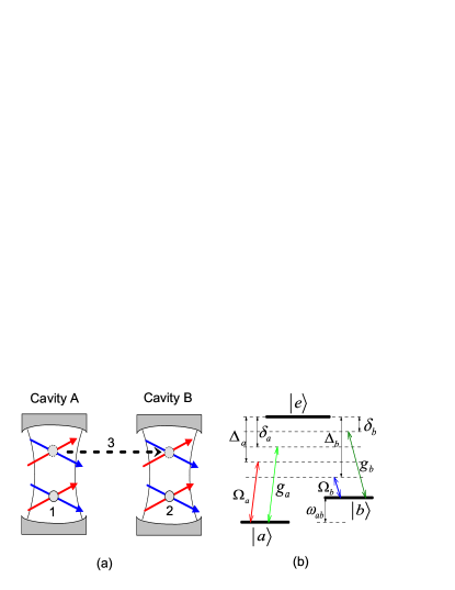
Figure 1: (Color online) (a) Schematic illustration for identification of unknown BDS based on the cavity QED system. The probe atom 3 first interacts with atom 1 in cavity A and then is sent to cavity B to interacts with atom 2. Each atom in the cavity is driven by two classical lasers. (b) Atomic levels and transitions.

To start the scheme, we pick up a pair of entangled atoms from the BDS ensemble and put them into the corresponding cavities. The probe atom 3 is sent into cavity A firstly. The Hamiltonian in cavity A can be written as follows,

$$H_{A} = \sum_{j=1,3}\omega_{e}|e\rangle_{j}\langle e|+\omega_{ab}|b\rangle_{j}\langle b|+\omega_{c}a^{\dagger}a$$ (24)

$$+(\Omega_{a}e^{-i\omega_{a}t}+g_{a}a)|e\rangle_{j}\langle a|$$

$$+(\Omega_{b}e^{-i\omega_{b}t}+g_{b}a)|e\rangle_{j}\langle b|,$$

where $\omega_{e}$ is the energy of $|e\rangle$ while $\omega_{ab}$ is the energy of $|b\rangle$, $\omega_{a}$ ($\omega_{b}$) is the frequency of the driver laser with Rabi frequency $\Omega_{a}$ ($\Omega_{b}$), and $a$ is the annihilation operator of the cavity.

By setting $\delta_{1}=\omega_{ab}-(\omega_{a}-\omega_{b})/2$, we switch to an interaction picture with respect to $H_{0}=\sum_{j=1,3}\omega_{e}|e\rangle_{j}\langle e|+(\omega_{ab}-\delta_{1})|b\rangle_{j}\langle b|+\omega_{c}a^{\dagger}a$. Under the large detuning condition $|\delta_{a}|,|\delta_{b}|,|\Delta_{a}|,|\Delta_{b}|\gg|g_{a}|,|g_{b}|,|\Omega_{a}|,|\Omega_{b}|$, where $\delta_{a}=\omega_{e}-\omega_{c}$, $\delta_{b}=\omega_{e}-\omega_{c}-\omega_{ab}+\delta_{1}$, $\Delta_{a}=\omega_{e}-\omega_{a}$, $\Delta_{b}=\omega_{e}-\omega_{b}-\omega_{ab}+\delta_{1}$, we can adiabatically eliminated the excited state $|e\rangle_{j}$ [20-23]. If there are no photons in the cavity and the detunings satisfy $|\delta_{a}-\Delta_{b}+g_{a}^{2}/\delta_{a}|,|\delta_{b}-\Delta_{a}+g_{a}^{2}/\delta_{a}|\gg|\Omega_{a}g_{b}/\Delta_{a}|,|\Omega_{b}g_{a}/\Delta_{b}|$ (we have assumed $g_{a}^{2}/\delta_{a}=g_{b}^{2}/\delta_{b}$), considering the subspace without real photons, we deduce the effective Hamiltonian as

$$H_{\mathrm{eff}}=\frac{2(J_{1}\sigma_{1}^{+}+J_{2}\sigma_{1}^{-})(J_{1}\sigma_{3}^{-}+J_{2}\sigma_{3}^{+})}{\delta_{a}-\Delta_{b}+g_{a}^{2}/\delta_{a}}+B(\sigma_{1}^{z}+\sigma_{3}^{z}),$$ (25)

where $\sigma_{i}^{+}=|b\rangle_{i}\langle a|$ and $\sigma_{i}^{-}=|a\rangle_{i}\langle b|$, the coefficients are given as

$$J_{1}=\frac{g_{a}\Omega_{b}}{2}(\frac{1}{\delta_{a}}+\frac{1}{\Delta_{b}}),$$ (26)

$$J_{2}=\frac{g_{b}\Omega_{a}}{2}(\frac{1}{\delta_{b}}+\frac{1}{\Delta_{a}}),$$ (27)

$$B = \frac{\Omega_{a}^{2}\Omega_{b}^{2}/4}{\delta_{a}-\delta_{b}}(\frac{1}{\Delta_{a}}+\frac{1}{\Delta_{b}})^{2}+\frac{\Omega_{b}^{2}g_{b}^{2}/4}{\delta_{b}-\Delta_{a}+g_{a}^{2}/\delta_{a}}(\frac{1}{\Delta_{b}}+\frac{1}{\delta_{b}})^{2}$$ (32)

$$-\frac{\Omega_{a}^{2}g_{a}^{2}/4}{\delta_{a}-\Delta_{a}+g_{a}^{2}/\delta_{a}}(\frac{1}{\Delta_{a}}+\frac{1}{\delta_{a}})^{2}$$

$$+\frac{1}{2}(\frac{\Omega_{b}^{2}}{\Delta_{b}}-\frac{\Omega_{a}^{2}}{\Delta_{a}}+\delta_{1}).$$

The effective magnetic field $B$ can be tuned to be very close to zero by varying $\delta_{1}$. For $\Omega_{b}=g_{b}\Omega_{a}(\frac{1}{\Delta_{a}}+\frac{1}{\delta_{b}})/[g_{a}(\frac{1}{\delta_{a}}+\frac{1}{\Delta_{b}})]$, we can get the final effective Hamiltonian as follows,

$$H_{xx}=\lambda_{x}\sigma_{1}^{x}\sigma_{3}^{x}.$$ (33)

where $\lambda_{x}=2J_{1}^{2}/(\delta_{a}-\Delta_{b}+g_{a}^{2}/\delta_{a})$. It is obvious to see that the unitary time-evolution operator $e^{-iH_{xx}t}$ is in accordance with the unitary operator $U_{13}^{1}$ at $t=\frac{(2n+1)\pi}{4\lambda_{x}},n=0,1,2...$, thus we realize the unitary operation $U_{13}$. To realize the operation $U_{23}^{2}$, we send the probe atom to cavity B, and drive atoms 2 and 3 with the same lasers as done in cavity A.

If we select the Rabi frequency as $\Omega_{b}=-g_{b}\Omega_{a}(\frac{1}{\Delta_{a}}+\frac{1}{\delta_{b}})/[g_{a}(\frac{1}{\delta_{a}}+\frac{1}{\Delta_{b}})]$, we can obtain

$$H_{yy}=\lambda_{y}\sigma_{1}^{y}\sigma_{3}^{y}.$$ (34)

where $\lambda_{y}=2J_{1}^{2}/(\delta_{a}-\Delta_{b}+g_{a}^{2}/\delta_{a})$. At time $t=\frac{(2n+1)\pi}{4\lambda_{y}},n=0,1,2...$, the time-evolution unitary operator $e^{-iH_{yy}t}$ coincides with the operator $U^{2}_{13}$. Then sent the probe atom into cavity B, we can realize the unitary operator $U^{2}_{23}$ by controlling the interaction time.

In order to realize the operations $U^{3}_{13}$ and $U^{3}_{23}$, we choose the laser frequencies as $\omega_{a}=\omega_{b}=\omega$. We switch to an interaction picture with respect to $H_{0}=\sum_{j=1,3}\omega_{e}|e\rangle_{j}\langle e|+(\omega_{ab}-\tilde{\delta}_{1})|b\rangle_{j}\langle b|+\omega_{c}a^{\dagger}a$, where the detuning $\tilde{\delta}_{1}$ is introduced to tune the effective magnetic field. Under the large detuning condition we can adiabatically eliminated the excited states. If there are no photons in the cavity and the detunings satisfy $|\delta_{a}-\Delta_{a}+g_{a}^{2}/\delta_{a}|,|\delta_{b}-\Delta_{b}+g_{a}^{2}/\delta_{a}|\gg|\Omega_{a}g_{a}/\Delta_{a}|,|\Omega_{b}g_{b}/\Delta_{b}|$ (assuming $g_{a}^{2}/\delta_{a}=g_{b}^{2}/\delta_{b}$), considering a subspace with no real photons we can obtain the following effective Hamiltonian,

$$H_{\mathrm{eff}} = \frac{2(\tilde{J}_{1}|a\rangle_{1}\langle a|+\tilde{J}_{2}|b\rangle_{1}\langle b|)(\tilde{J}_{1}|a\rangle_{2}\langle a|+\tilde{J}_{2}|b\rangle_{2}\langle b|)}{\delta_{a}-\Delta_{a}+g^{2}_{a}/\delta_{a}}$$ (37)

$$+\tilde{B}(\sigma_{1}^{z}+\sigma^{z}_{3}),$$

where $\sigma^{z}_{i}=|b\rangle_{i}\langle b|-|a\rangle_{i}\langle a|$, and the coefficients are given as follows,

$$\tilde{J}_{1}=\frac{\Omega_{a}g_{a}}{2}(\frac{1}{\Delta_{a}}+\frac{1}{\delta_{a}}),$$ (38)

$$\tilde{J}_{2}=\frac{\Omega_{b}g_{b}}{2}(\frac{1}{\Delta_{b}}+\frac{1}{\delta_{b}}),$$ (39)

$$\tilde{B} = \frac{1}{2}(\frac{\Omega^{2}_{b}}{\Delta_{b}}+\tilde{\delta}_{1}-\frac{\Omega^{2}_{a}}{\Delta_{a}})+\frac{1}{2}[\frac{\Omega_{b}^{2}g_{a}^{2}/4}{\delta_{a}-\Delta_{b}+g_{a}^{2}/\delta_{a}}(\frac{1}{\delta_{a}}+\frac{1}{\Delta_{b}})^{2}$$ (44)

$$-\frac{\Omega_{a}^{2}g_{b}^{2}/4}{\delta_{b}-\Delta_{a}+g_{a}^{2}/\delta_{a}}(\frac{1}{\delta_{b}}+\frac{1}{\Delta_{a}})^{2}]$$

$$+\frac{\Omega_{a}^{2}\Omega_{b}^{2}/4}{\Delta_{a}-\Delta_{b}}(\frac{1}{\Delta_{a}}+\frac{1}{\Delta_{b}})^{2}.$$

The effective magnetic field can be tuned to zero by varying $\tilde{\delta}_{1}$. For $\Omega_{b}=-\Omega_{a}g_{a}(\frac{1}{\Delta_{a}}+\frac{1}{\delta_{a}})/[g_{b}(\frac{1}{\Delta_{b}}+\frac{1}{\delta_{b}})]$, we can obtain the following effective Hamiltonian,

$$H_{zz}=\lambda_{z}\sigma_{1}^{z}\sigma_{3}^{z},$$ (45)

where $\lambda_{z}=2\tilde{J}_{1}/(\delta_{a}-\Delta_{a}+g_{a}^{2}/\delta_{a})$. It is obvious to see that the time-evolution unitary operator $e^{-iH_{zz}t}$ coincides with $U_{13}^{3}$ at time points $t=\frac{(2n+1)\pi}{4\lambda_{z}}$ $(n=0,1,2,...)$. Thus we have realized the operation $U^{3}_{13}$ in cavity A, in the same way we can realize the operation $U^{3}_{23}$ in cavity B by sending the probe atom into cavity B.

To confirm the validity of our approximation, we numerically simulate the dynamics generated by the full Hamiltonian and compare it to the the dynamics generated by the effective Hamiltonian. In Fig. 2(a), we have plotted the time evolution of $\langle\sigma_{3}^{z}\rangle$. The numerical results show that the performance of $\langle\sigma_{3}^{z}\rangle$ under the full Hamiltonian and that under $H_{xx}$ agree with each other reasonably well. Similar agreement can also be seen in Fig. 2(b) and (c). Therefore, our effective model is valid.

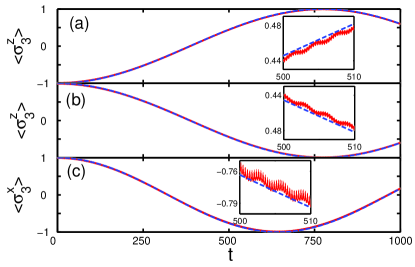
Figure 2: (Color online) Time evolutions of atom 3 calculated using full Hamiltonian (dashed blue line) and effective Hamiltonians (solid red line). The effective Hamiltonians for (a), (b), and (c) are $H_{xx}$, $H_{yy}$, and $H_{zz}$, respectively. The initial states are chosen as $0.5(|a\rangle_{1}\langle a|+|b\rangle_{1}\langle b|)\otimes|a\rangle_{3}\langle a|$ for (a) and (b), and $0.25(|a\rangle_{1}\langle a|+|b\rangle_{1}\langle b|)\otimes(|a\rangle+|b\rangle)_{3}(\langle a|+\langle b|)$ for (c). The parameters are chosen as $g_{a}=1$, $\Omega_{a}=5g_{a}$, $\delta_{a}=102g_{a}$, $\delta_{b}=122g_{a}$, $\Delta_{a}=120g_{a}$, and $\Delta_{b}=100g_{a}$ for (a) and (b); $g_{a}=1$, $\Omega_{a}=5g_{a}$, $\delta_{a}=102g_{a}$, $\delta_{b}=122g_{a}$, $\Delta_{a}=100g_{a}$, and $\Delta_{b}=120g_{a}$ for (c). The inset shows the behaviors of the two curves in detail with time $t\in[500,510]$ (in units of $1/g_{a}$).

So far, we have realized all the unitary operations described by Eqs. (17)-(19) in the cavity QED system. Since the qubits are encoded in the ground atomic states and there is no real photons in the cavity, this experimental scenario is robust against the dissipative effects.

Here we give a brief discussion on the experimental feasibility of the presented scheme. For an experimental implementation, the effective coupling strengths $\lambda_{x}$, $\lambda_{y}$, and $\lambda_{z}$ should be much larger than the cavity leaky rate $\Gamma_{C}$ and the atomic spontaneous rate $\Gamma_{E}$. This requirements can be satisfied in microcavities which have a small volume and thus a high quality factor. Suitable candidates for the present proposal are, for example, the microtoroidal cavities which has cooperativity factor $g^{2}/(\Gamma_{C}\Gamma_{E})\sim 10^{7}$ and the ratio $g/\Gamma_{E}\sim 10^{3}$ [23,24], where $g$ is defined by $g=\mathrm{max}(g_{a},g_{b})$. Thus our scheme is feasible with current available systems.

IV Conclusion

In conclusion, we have presented a scheme for nondestructive identifying unknown BDS by measuring the probe qubits. This scheme is implemented in three steps. In each step we can build an equation between the unknown coefficients of the BDS and the observable of the probe qubit. Combining the three equations we can calculate the parameters. Moreover, at the end of each step, the BDS ensemble remains in the initial state, therefore it is not polluted by the identification processing. We also consider the experimental realization of the scheme in the cavity QED system. By selecting appropriate Rabi frequencies of the driving lasers, we can realize the corresponding unitary operations, respectively. Our scheme is feasible with the current techniques.

V Acknowledgement

This work was supported by the National Natural Science Foundation of China, under Grants No. 10805007 and No. 10875020, and the Doctoral Startup Foundation of Liaoning Province.

References

- (1) T. Pellizzari, S. A. Gardiner, J. I. Cirac, and P. Zoller, Phys. Rev. Lett. 75, 3788 (1995).
- (2) J. I. Cirac, P. Zoller, H. J. Kimble, and H. Mabuchi, Phys. Rev. Lett. 78, 3221 (1997).
- (3) S. J. van Enk, J. I. Cirac, and P. Zoller, Phys. Rev. Lett. 78, 4293 (1997).
- (4) C. H. Bennett, G. Brassard, C. Crépeau, R. Jozsa, A. Peres and W. K. Wootters, Phys.Rev.Lett. 70, 1895 (1993).
- (5) C. Bouwmeester, J.W. Pan, K. Mattle, M. Elbl, H. Weinfurter, and A. Zeilinger, Nature (London) 390, 575 (1997).
- (6) F. Verstraete and H. Verschelde, Phys. Rev. Lett. 90, 097901 (2003).
- (7) C. H. Bennett, G. Brassard, S. Popescu, B. Schumacher, J. A. Smolin, and W. K. Wootters, Phys. Rev. Lett. 76, 722 (1996).
- (8) Z. W. Wang, X. F. Zhou, Y. F. Huang, Y. S. Zhang, X. F. Ren, and G. C. Guo, Phys. Rev. Lett. 96, 220505 (2006).
- (9) M. Koashi and N. Imoto, Phys. Rev. Lett. 77, 2137 (1996).
- (10) M. D. Lang and C. M. Caves, Phys. Rev. Lett. 105, 150501 (2010).
- (11) L. Mazzola, J. Piilo, and S. Maniscalco, Phys. Rev. Lett. 104, 200401 (2010).
- (12) J. S. Xu, X. Y. Xu, C. F. Li, C. J. Zhang, X. B. Zou, and G. C. Guo, Nat. Commun. 1, 7 (2010).
- (13) L. X. Cen, N. J. Wu, F. H. Yang, and J. H. An, Phys. Rev. A 65, 052318 (2002).
- (14) C. F. Roos, G. P. T. Lancaster, M. Riebe, H. Hffner, W. Hnsel, S. Gulde, C. Becher, J. Eschner, F. Schmidt-Kaler, and R. Blatt, Phys. Rev. Lett. 92, 220402 (2004).
- (15) R. Blatt and D. Wineland, Nature 453, 1008 (2008).
- (16) J. P. Home, M. J. McDonnell, D. M. Lucas, G. Imreh, B. C. Keitch, D. J. Szwer, N. R. Thomas, S. C. Webster, D. N. Stacey, and A. M. Steane, New J. Phys. 8, 188 (2006).
- (17) M. Koschorreck, M. Napolitano, B. Dubost, and M. W. Mitchell, Phys. Rev. Lett. 105, 093602 (2010).
- (18) J. S. Jin, C. S. Yu, P. Pei, and H. S. Song, Phys. Rev. A 82, 042112 (2010).
- (19) M. J. Woolley, A. C. Doherty, and G. J. Milburn, Phys. Rev. B 82, 094511 (2010).
- (20) D. F. V. James and J. Jerke, Can. J. Phys. 85, 625 (2007).
- (21) M. J. Hartmann, F. G. S. L. Brando, and M. B. Plenio, Phys. Rev. Lett. 99, 160501 (2007).
- (22) L. Zhou, W. B. Yan, and X. Y. Zhao, J. Phys. B: At. Mol. Opt. Phys. 42, 065502 (2009).
- (23) S. M. Spillane, T. J. Kippenberg, K. J. Vahala, K. W. Goh, E. Wilcut, and H. J. Kimble, Phys. Rev. A 71, 013817 (2005).
- (24) Z. X. Chen, Z. W. Zhou, X. X. Zhou, X. F. Zhou, and G. C. Guo, Phys. Rev. A 81, 022303 (2010).