Wigner-PDC description of photon entanglement as a local-realistic theory

Abstract

(Revised, added references to recent tests)

The Wigner picture of Parametric Down Conversion (works by Casado et al) can be interpreted as a local-realistic formalism, without the need to depart from quantum mechanical predictions at any step, at least for the relevant subset of QED-states. This involves reinterpreting the expressions for the detection probabilities, by means of an additional mathematical manipulation; such manipulation seemingly provides enough freedom to guarantee consistency with the expectable, experimentally testable behavior of detectors, that being nevertheless an unnecessary requirement in relation to our main results, of a purely mathematical nature. We also include an overview of the consequences of such results in relation to typical Bell experiments.

I Previous notes on recent non-locality tests

On the test of Giustina et al, 2015 Giustina2015 :

This is a PDC-based experiment where the estimated ”detection efficiencies” are, very probably, not significant because they are simply not well evaluated: the relevant parameter is a quotient, the denominator being a detection rate in a particular setting, the numerator being a proper average of the detection rates for each polarization at the other arm, conditioned to one obtained in the first… it seems that here the test only records or takes into account one of those two last rates -just one detector after each polarizer instead of the necessary two-; rates of detection in just one of the polarizations may not be (and I claim they will be proven not to be, if given the chance to) statistically significant of what one would obtain if both exit channels of the polarizer were detected, recorded: that is the crucial point in this so-called ”detection loophole” (I use the inverted commas as the whole of the approach I advocate here suggests that they are not substantially diminisehd by any ”detection efficiency”, but actually stand simply for the proper detection rates predicted by an underlying wave-like theory).

And once here let me ask: why would we not once and for all estimate those rates in the best possible way (with both detectors at each end)? As far as the information provided here goes, one cannot say this does closes any ”detection loophole”.

On the tests of Hensen et al, 2015/2016 Hensen2015 ; Hensen2016 :

How here is so readily stated that there is no ”detection loophole” remains an obscure, unsolvable mystery to me: regardless of the sophistication of the photon generation method (customarily Parametric Down Conversion, here another one based on a previous “entanglement” of the spins of two massive particles), what we have at the end is, as usual, two light signals travelling to two remote measurement settings (polarizer-detector) and everything said in the paragraph above applies exactly the same, taking this time into account the rate limits for the inequality tested, the CHSH one.

The first test has been followed by another one where some technical aspects regarding other loopholes are polished: these other ”loopholes” are not addresed here as in the opinion of the author they are just that, mere ”loopholes”; far beyond that, the detection loophole -and all that is related to it, ”enhancement” and so on- is clear evidence that the particle model with which these tests are modeled may be useful on a first approximation, but not subtle enough to describe the real physics going on underneath, a physics that ultimately excludes -how could it not?- all quantum states that are not compatible with well defined, pre-existing probability density functions for the results of all the measurements that can be performed upon the system: local-realism.

And once again here, there is ONLY ONE WAY to be sure of what is happening in these tests: to measure everything, compute all the rates, exhaustively, not just a conveniently chosen subensemble of the things one can observe in the laboratory so that one or other Bell inequality -and/or its additional assumptions- seems to be violated.

II Introduction

The Wigner picture of Quantum Optics of photon-entanglement generated by Parametric Down Conversion PDC_explanation was developed already some decades ago in a series of papers pdc1 ; pdc2 ; pdc3 ; pdc4 ; pdc5 ; pdc6 ; pdc7 ; more recently, the approach has been revitalized producing another stream of very interesting results pdc8 ; pdc9 ; pdc_2014 ; pdc_2015 ; pdc_2018 ; pdc_2019 .

Starting from an stochastic electrodynamical description (hence, based on continuous variables: electromagnetic fields defined at each and every point of space), by use of the so-called Wigner transformation KimNoz this model acquires a form where all expectation values depend on a probability distribution (hence one objectively defined) for the value of those fields in the vacuum.

Such a picture clearly differs from the one that is usually assumed in the field of Quantum Information (QInf), based on a discrete description of light (particles) and not on a wave-like model where photons could be perhaps be understood as the abstraction exclusively related to the “detection events”, indeed the only directly observable item for either the conventional (particle) model or our alternative (wavelike) one here. In relation to this last, let us remark that we do not at any point need the unprobable phenomenom of a “wave-packet” somehow managing to remain spatially and temporarily confined: all we need is a distribution of the values of the fields over the space-time continuun. That, and the pressence of a random background -whether that is the quantum electrodynamical one or another with adequate properties is indeed indifferent to most of what we will say here-, a vacuum Zero-Point field (ZPF). Those two elements, let us insist, are all we need: fields defined at every point of space, including a random, background component.

Once here, some differences between the two pictures become obvious even at the most preliminary, qualitative analysys: for instance, in this wave-like model the empty polarization channels at either of the exits of a polarizing beam splitter (PBS) will become filled with random components of that vacuum Zero-Point field (ZPF); such random components can for instance give rise to the enhancement of the detection probability if the overall intensity arrived at the detector is as a result increased: see note WignerPDC_enhancement . This comes up as a big difference with the customary model of the set polarizer-detector is treated just as a “black box”, blocking or just letting it go but always without the introduction of any additional noise or “information”.

It is then clear that the two models are not only internally different but they can also give rise to different predictions, and in particular that the Wigner-PDC framework offers considerably more “room” to accomodate physical phenomena that its conventional counterpart: for instance, the possibility of enhancement of the detection probability at a polarizer, or simply the appearance of a variable probability at the detector, dependent on the incoming intensity, something that one cannot explain in the customary particle-like picture if it is not through the inclusion of some external, artificially tuned “detection efficiencies” in the model -precisely our point that the low value of those efficiencies should not be blamed on technological limitations alone.

The Wigner-PDC framework provides an alternative, local-realistic explanation of the results of many typically quantum experiments, the result of a measurement depending on (and only on) the set of hidden variables (HV) inside its light cone: in this case, both the signal propagating from the source and the additional noise introduced by the ZPF at intermediate devices and detectors. Within a first series of published papers pdc1 ; pdc2 ; pdc3 ; pdc4 ; pdc5 ; pdc6 ; pdc7 those experiments included: frustrated two photon creation via interference pdc1 ; induced coherence and indistinguishableness in two-photon interference pdc1 ; pdc2 ; Rarity and Tapster’s 1990 experiment with phase-momentum entanglement pdc2 ; Franson’s (original, 1989) experiment pdc2 ; quantum dispersion cancellation and Kwiat, Steinberg and Chiao’s quantum eraser pdc3 .

From a most recent series pdc8 ; pdc9 ; pdc_2014 ; pdc_2015 ; pdc_2018 ; pdc_2019 we can add, on one side and amongst quantum cryptography experiments based on PDC, two-qubit entanglement and cryptography pdc8 and quantum key distribution and eavesdropping pdc8 ; on the other, an interpretation for the experimental partial measurement of the Bell states generated from a single degree of freedom (polarization) pdc9 , as well as polarization-momentum hyperentanglement pdc_2014 , entanglement swapping and teleportation pdc_2015 and complete one-photon polarization-momentum Bell-state analysis pdc_2018 ; most recently some more results have been obtained in relation to optical quantum communication experiments pdc_2019

As a ”local realistic” theory, due to its the mathematical structure based on well defined “a priori” probability density functions for the local hidden values (the distribution of fields), it is obvious that this formalism must give rise to predicted detection rates (the low values of which in some other context are customarily associated to a detection efficiencies), are naturally bound to remain within the limits (what other call “critical detection rates”) where it is already well acknowledged that such an explanation may exist; moreover, and this is a crucial point, those limits would appear as just natural consequences of the theory: they are simply limiting values of detection rates -in particular conditional joint detection rates- for states of light generated from a non-linear mix of a classical signal (the laser) with a set of random components (the vacuum). However, that local-realistic interpretation was so far not devoid of other difficulties, in particular related to the detection model (so far merely a one-to-one counterpart with Glauber’s original expressions detection ): as a result of the normal order of operators, there average intensity due to vacuum fluctuations is “subtracted”, a subtraction that seems to introduce problems related to the appearance of what could be interpreted as “negative probabilities”.

That last is the issue that interests us here, one that, as to be expected, did motivate the proposal of several modifications upon the expressions for the detection probabilities: for instance, as early as in pdc4 , “our theory is also in almost perfect one-to-one correspondence with the standard Hilbert-space theory, the only difference being the modification in the detection probability that we proposed in relation…”.

Such modifications ranged from the mere inclusion of temporal and spatial integration pdc4 to the proposal of much more complicated functional dependencies pdc7 ; W_LHV_02 ; MS2008 , all of them seeming to pose their own problems; for instance in W_LHV_02 , a departure from the quantum predictions at low or high intensities, experimentally disproved for instance in Brida_et_al02 . Our route here is a different one however: we do not propose any modification of the initial expressions for the detection probabilities (in one-to-one correspondence with the initial quantum electrodynamical model), but just explore the possibility of performing some convenient mathematical manipulation that casts them in a form consistent with the axioms of probability, hence one consistent with local-realism.

Following for instance pdc4 ; pdc_2019 (see also detection ), single detection probabilities can be expressed as

$$P_{i} \propto \langle I_{i}-I_{0,i}\rangle$$ (1)

$$= \int_{\alpha,\alpha^{*}}(I_{i}(\alpha,\alpha^{*})-I_{0,i})\ W(\alpha,\alpha^{*})\ d\alpha d\alpha^{*},$$

and double -coincident- detections obey, at least whenever there are conditions of space-like separation (see for instance pdc4 ; pdc_2019 ), the following expression

$$P_{i,j} \propto \int_{\alpha,\alpha^{*}}(I_{i}(\alpha,\alpha^{*})-I_{0,i})\cdot(I_{j}(\alpha,\alpha^{*})-I_{0,j})$$ (2)

$$\quad\quad\quad\quad\quad\quad\quad\quad\quad\times\ W(\alpha,\alpha^{*})\ d\alpha d\alpha^{*},$$

where $\alpha,\alpha^{*}$ are vacuum amplitudes of the (relevant set of) frequency modes note_modes at the entrance of the crystal, $W(\alpha,\alpha^{*})$ is obtained as the Wigner transform of the vacuum state, $I_{i}(\alpha,\alpha^{*})$ is the field intensity (for that mode) and $I_{0,i}$ the mean intensity due to the vacuum amplitudes, both at the entrance of the $i$-th detector (see note_modes ):

$$I_{0}=\int_{\alpha,\alpha^{*}}I_{0}(\alpha,\alpha^{*})\ W(\alpha,\alpha^{*})\ d\alpha d\alpha^{*}.$$ (3)

The last three expressions would in principle allow us to identify the vacuum amplitudes with a vector of hidden variables $\lambda\in\Lambda$ ($\Lambda$ is the space of events or probabilistic space), with an associated density function $\rho(\lambda)$,

$$\lambda \equiv \alpha,\alpha^{*},$$ (4)

$$\rho(\lambda) \equiv W(\alpha,\alpha^{*}).$$ (5)

Now, for instance in pdc4 it is already acknowledged that (1)–(2) cannot, because of the possible negativity of the difference $I_{i}(\alpha,\alpha^{*})-I_{0,i}$, be written as

$$P_{i} = \int_{\Lambda}{P_{i}(det|\lambda)\ \rho(\lambda)\ d\lambda},$$ (6)

$$P_{i,j} = \int_{\Lambda}{P_{i,j}(det|\lambda)\ \rho(\lambda)\ d\lambda},$$

(7)

where naturally $P_{i}(det|\lambda),P_{i,j}(det|\lambda)$ should stay positive (or zero) always. This last is our point of departure: in this paper we propose a reinterpretation of the former marginal and joint detection probabilities based on a certain manipulation of expressions (1)–(2).

The paper is organized as follows. In Sec.III we will consider a setup with just a source and two detectors; once that is understood, the interposition of other devices between the source and the detectors poses no additional conceptual difficulty though it is nevertheless convenient to address it in some detail: this will be done in Sec. IV. The calculations in these two sections find support on the proofs provided in Appendix .1, and stand for our main result in this paper. Sec. V explores the question of “$\alpha$-factorability” in the model, not only from the mathematical point of view but also providing some more physical insights on its implications.

Up to that point the novel points of the paper are made and its results are self-contained; it is nevertheless natural to extend our analysis to some of their further implications (amongst these, the consequences for Bell tests of local-realism, and also a recent related proposal), in Sec. VI, where we also include a preliminary approach to questions regarding the physics of the real detectors. Finally, overall conclusions are presented in Sec. VII, and some supplementary material is provided in Appendix .2, which may not only help make the paper self-contained but perhaps also contribute to clarify some of the questions addressed in this paper.

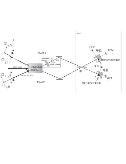
Figure 1: Wigner-PDC description for a typical experiment, including photon pair generation, polarizing beam splitters (PBS) and detectors. Only relevant inputs of Zero-Point vacuum field (ZPF) are represented in the picture: “relevant” can be understood, in a classical wavelike approach, as “necessary to satisfy energy-momentum conservation” for the (set of) frequency modes of interest; in a purely quantum electrodynamical framework we would be talking about conservation of the commutation relations at the empty exit channels of the devices. Besides, those new ZPF components introduced at the empty exit channels of PBS’s 1 and 2 can alter the detection probability for the signal arriving to the detectors (for instance giving rise to its “enhancement”); that signal is on the other hand determined (amongst other hidden variables) by the ZPF components entering the crystal. Figure: courtesy of A. Casado.

III Reinterpreting detection probabilities

Our aim is to adopt here an approach that is deliberately as abstract as it can be chosen to be, because what we are concerned about is an (apparent) problem of the mathematical structure of the theory, rather than other details regarding its connection with physical reality which should in principle be addressed at another stage of the investigation. Nevertheless, of course for the sake of credibility some of these details need to be brought up, and so we will do when necessary.

We now propose a reinterpretation of expressions (1)–(2) which is based on the idea that it is legitimate to play with internal degrees of freedom of a theory, as far as its observable predictions remain all of them invariant to these transformations. We intend to make a progressive exploration of the possible consistency conditions, from less to more demanding, but we advance that in no way this threatens the validity of our main result here, as we will be able to provide proof of the existence of the required solution for all of them.

III.1 Single detections

Knowing that the following equality holds (from here on we drop detector indexes when unnecessary), for some real constant $K_{(m)}$ (“marginal”),

$$K_{(m)}\int_{\alpha,\alpha^{*}}(I(\alpha,\alpha^{*})-I_{0})\ W(\alpha,\alpha^{*})\ d\alpha d\alpha^{*}$$

$$\quad\quad\quad\quad\quad\quad\quad\quad=\int_{\Lambda}{P(det|\lambda)\ \rho(\lambda)\ d\lambda},$$ (8)

we realize we do not need to assume

$$P(det|\lambda) \equiv K_{(m)}\cdot(I(\alpha,\alpha^{*})-I_{0}),$$ (9)

as a necessary, compulsory choice; it would be enough to find some $f(x)\geq 0$, satisfying

$$K_{(m)}\int_{\alpha,\alpha^{*}}(I(\alpha,\alpha^{*})-I_{0})\ W(\alpha,\alpha^{*})\ d\alpha d\alpha^{*}$$

$$\quad\quad\quad\quad\quad\quad=\int_{\alpha,\alpha^{*}}f(I(\alpha,\alpha^{*}))\ W(\alpha,\alpha^{*})\ d\alpha d\alpha^{*},$$

(10)

so we can then safely identify

$$P(det|\lambda) \equiv f(I(\alpha,\alpha^{*})),$$ (11)

with $f(I(\alpha,\alpha^{*}))\geq 0$, $\forall I(\alpha,\alpha^{*})$. This last is nothing but solving a linear system with only one restriction and an infinite number of free parameters, whose subspace of solutions intersects the region $0\leq f(I(\alpha,\alpha^{*}))\leq 1$ $\forall\alpha,\alpha^{*}$: see Appendix .1.

III.2 Joint detections

From the perspective of our approach and regarding joint detections, it is not very clear which are really the minimum conditions of consistence that one would have to enforce; in order to proceed with the maximum generality, let us simply define, for detectors $i,j$ and a constant $K_{(j)}$ (“joint”), a new function $\Gamma(x,y)$, so that

$$K_{(j)}\int(I_{i}(\alpha,\alpha^{*})-I_{0,i})\cdot(I_{j}(\alpha,\alpha^{*})-I_{0,j})$$

$$\quad\quad\quad\quad\quad\quad\quad\quad\quad\quad\quad\quad\quad\quad\times\ W(\alpha,\alpha^{*})\ d\alpha d\alpha^{*}$$

$$\quad\quad=\int\Gamma(I_{i}(\alpha,\alpha^{*}),I_{j}(\alpha,\alpha^{*}))\ W(\alpha,\alpha^{*})\ d\alpha d\alpha^{*},$$

(12)

which we will now attempt to interpret as

$$P_{i,j}(det|\lambda) \equiv \Gamma(I_{i}(\alpha,\alpha^{*}),I_{j}(\alpha,\alpha^{*})).$$ (13)

Of course, at a first look it seems very desirable to guarantee that the detection probabilities depend solely on the amount of intensity at the entrance of each detector; hence it would seem natural to add the condition

$$\Gamma(I_{i}(\alpha,\alpha^{*}),I_{j}(\alpha,\alpha^{*}))=f(I_{i}(\alpha,\alpha^{*}))\cdot f(I_{j}(\alpha,\alpha^{*})),$$

(14)

i.e., some “factorability” on the incoming intensities. Again, while such an additional condition seems necessary in order to preserve the “physical interpretability” of the “inner structure” of the theory, it is not at all something necessary from the point of view of its observable predictions, as long as these remain invariant; as we will see later, $I_{j}(\alpha,\alpha^{*})$ may not only be unobservable as corresponds to a particular realization of the random fields… it may also happens that it does not actually represent a real intensity, but just an average promediated over another relevant random variable.

In Appendix .1 we have shown that it is always possible to find some suitable $\Gamma$ satisfying all necessary conditions to be interpreted as a probability distribution and consistent with the observable prediction of the theory regarding joint detections, eq. (2); and, furthermore, that a solution can be found satisfying also (14).

As said, our choice here is to proceed without loss of generality: for this purpose, it is convenient to redefine now $\alpha\equiv\alpha,\alpha^{*}$, as well as

$$\hat{f}_{i}(\alpha) \equiv f(I_{i}(\alpha)),$$ (15)

$$\hat{\Gamma}_{i,j}(\alpha) \equiv \Gamma(I_{i}(\alpha),I_{j}(\alpha)).$$ (16)

where we now assume that in general,

$$\Gamma_{i,j}(\alpha)\neq f_{i}(\alpha)\cdot f_{j}(\alpha),$$ (17)

The absence of factorability on the $\alpha$’s may come perhaps as a surprise to some, given than Clauser-Horne factorability CH74 on the hidden variable $\lambda$ is usually taken for granted; this is a mistake factorability , that we have tried to clarify in Appendix .2.

IV Adding intermediate devices: polarizers, PBS’s…

Once we place one or more devices between the crystal and the detectors, typically polarizers, polarizing beam splitters (PBS) or other devices to allow polarization measurements (such as in Fig. 1), in general we cannot any longer describe the fields between both with only one set $\{\alpha\}$ of mode-amplitudes; we need to redefine our $\alpha$’s as now associated to a particular position $\mathbf{r}$ (they do not any longer determine a frequency mode for all space note_modes ). Hence, we will now have

$$\alpha(\mathbf{r})\equiv\{\alpha_{\mathbf{k},\gamma}(\mathbf{r}),\alpha_{\mathbf{k},\gamma}^{*}(\mathbf{r})\},$$ (18)

and, letting $\mathbf{r}_{s}$ be the position of the source (the crystal), and $\mathbf{r}_{i}$ the position of the $i$-th polarizer or PBS (or any other intermediate device), we will also redefine

$$\alpha_{s} \equiv \alpha(\mathbf{r}_{s}),\quad\alpha_{i}\equiv\alpha(\mathbf{r}_{i}),$$ (19)

with $\alpha_{i}$ including the relevant amplitudes at the (empty) exit channels of that $i$-th intermediate device. With $\alpha_{s},\alpha_{i}$ corresponding each to (a set of) modes with different (sets of relevant) wavevectors $\{\mathbf{k}_{s}\}$ and $\{\mathbf{k}_{i}\}$ note_wvectors , we can then regard them as two (sets of) statistically independent random variables, with all generality. The intensity at the entrance of detector $i$-th will therefore depend now not only on $\alpha_{s}$ but also on $\alpha_{i}$:

$$P_{i} \propto \langle I_{i}(\alpha_{s},\alpha_{i})-I_{0,i}\rangle$$

$$= \int_{\alpha_{s}}\int_{\alpha_{i}}(I_{i}(\alpha_{s},\alpha_{i})-I_{0,i})\ W(\alpha_{s})\ W(\alpha_{i})\ d\alpha_{s}d\alpha_{i}.$$

(20)

Once more, something like that can always be rewritten (see former section), for some suitable and positively defined $f^{\prime}(x)$, as

$$P_{i} = \int_{\alpha_{s}}\int_{\alpha_{i}}f^{\prime}(I_{i}(\alpha_{s},\alpha_{i}))\ W(\alpha_{s})\ W(\alpha_{i})\ d\alpha_{s}d\alpha_{i}.$$

Integrating on $\alpha_{i}$ we would obtain

$$P_{i} = \int_{\alpha_{s}}\hat{f}^{\prime}_{i}(\alpha_{s})\ W(\alpha_{s})\ d\alpha_{s},$$ (22)

from where we define a new function $\hat{f}^{\prime}_{i}(\alpha_{s})$. On the other hand, for joint detections we would have

$$P_{i,j} \propto \int_{\alpha_{s}}\int_{\alpha_{i}}\int_{\alpha_{j}}(I_{i}(\alpha_{s},\alpha_{i})-I_{0,i})\cdot(I_{j}(\alpha_{s},\alpha_{j})-I_{0,j})$$

$$\quad\quad\quad\quad\quad\times\ W(\alpha_{s})\ W(\alpha_{i})\ W(\alpha_{j})\ d\alpha_{s}d\alpha_{i}d\alpha_{j},$$

(23)

which again can always be rewritten (again see former section), for some positively defined $\Gamma^{\prime}(x,y)$, as

$$P_{i,j} = \int_{\alpha_{s}}\int_{\alpha_{i}}\int_{\alpha_{j}}\Gamma^{\prime}(I_{i}(\alpha_{s},\alpha_{i}),I_{j}(\alpha_{s},\alpha_{j}))$$

$$\quad\quad\quad\quad\quad\times\ W(\alpha_{s})\ W(\alpha_{i})\ W(\alpha_{j})\ d\alpha_{s}d\alpha_{i}d\alpha_{j},$$

and integrating on $\alpha_{i},\alpha_{j}$ we would obtain

$$P_{i,j} = \int_{\alpha_{s}}\hat{\Gamma}^{\prime}_{i,j}(\alpha_{s})\ W(\alpha_{s})\ d\alpha_{s},$$ (25)

from where we can again define yet another new probability density function $\hat{\Gamma}^{\prime}_{i,j}(\alpha_{s})$.

It is interesting for the sake of clarity to compare the two situations: with (primed functions) and without polarizers (unprimed). It is easy to see that, because the detector only sees the intensity at its entrance channel, clearly (we drop the “s” subscript for simplicity),

$$f^{\prime}(x) = f(x),\quad\forall x,$$ (26)

$$\Gamma^{\prime}(x,y) = \Gamma(x,y),\ \forall x,y.$$ (27)

while, in consistency with our approach, in general $\hat{f}^{\prime}_{i}(\alpha)\neq\hat{f}_{i}(\alpha)$, as well as $\hat{\Gamma}^{\prime}_{i,j}(\alpha)\neq\hat{\Gamma}_{i,j}(\alpha)$.

V On non-factorability

V.1 Mathematical analysis

Let us go back to the case with just the source and the detectors; we will soon see the following does nevertheless also apply when polarizers or other devices are added to the setup, just the same. According to our reasonings in App. .2, and using (15)–(16), we now realize that there is no way to avoid

$$\hat{\Gamma}_{i,j}(\alpha)=\hat{f}_{i}(\alpha)\cdot\hat{f}_{j}(\alpha),$$ (28)

unless we introduce some additional dependence of the kind $\hat{f}(\alpha)\rightarrow\hat{\hat{f}}(\alpha,\mu)$, so that then

$$\hat{\hat{\Gamma}}_{i,j}(\alpha,\mu)\neq\hat{\hat{f}}_{i}(\alpha,\mu)\cdot\hat{\hat{f}}_{j}(\alpha,\mu),$$ (29)

where we add a second “hat” to avoid an abuse of notation, and where $\mu$ stands for a new set of random variables. This $\hat{\hat{f}}(\alpha,\mu)$ should be interpreted as a detection probability conditioned to the new vector of random variables $\mu$, i.e,

$$\hat{\hat{f}}(\alpha,\mu)\equiv P(det|\alpha,\mu).$$ (30)

We will impose further demands on $\hat{\hat{f}}(\alpha,\mu)$, defining

$$\hat{\hat{f}}(\alpha,\mu)\equiv f(I(\alpha,\mu)),$$ (31)

something forced by strictly physical arguments: the choice $f(I(\alpha,\mu))$ must prevail over other possible ones - for instance $f(I(\alpha),\mu)$ - due to the need to respect the dependence of the probabilities of detection (conditioned to $\alpha$ or not) alone on the intensity that arrives to the detector, and nothing else.

Now, with the density function $\rho_{\mu}(\mu)$, we could write

$$P(det|\alpha) = \int_{\mu}P(det|\alpha,\mu)\ \rho_{\mu}(\mu)\ d\mu,$$ (32)

$$P_{i,j}(det|\alpha) = \int_{\mu}P_{i,j}(det|\alpha,\mu)\ \rho_{\mu}(\mu)\ d\mu,$$ (33)

allowing us to recover our former definitions (15)–(16):

$$\hat{f}(\alpha)\equiv P(det|\alpha),$$ (34)

$$\hat{\Gamma}_{i,j}(\alpha)\equiv P_{i,j}(det|\alpha).$$ (35)

For joint detections, the additional variable $\mu$ is particularly relevant because, we will always have that while

$$P_{i,j}(det|\alpha,\mu)=P_{i}(det|\alpha,\mu)\cdot P_{j}(det|\alpha,\mu),$$ (36)

in general

$$P_{i,j}(det|\alpha)\neq P_{i}(det|\alpha)\cdot P_{j}(det|\alpha),$$ (37)

or we could equivalently say that while necessarily

$$\hat{\hat{\Gamma}}_{i,j}(\alpha,\mu)=\hat{\hat{f}}_{i}(\alpha,\mu)\cdot\hat{\hat{f}}_{j}(\alpha,\mu),$$ (38)

in general

$$\hat{\Gamma}_{i,j}(\alpha)\neq\hat{f}_{i}(\alpha)\cdot\hat{f}_{j}(\alpha),$$ (39)

where of course

$$\hat{\Gamma}_{i,j}(\alpha)=\int_{\mu}\hat{\hat{f}}_{i}(\alpha,\mu)\cdot\hat{\hat{f}}_{j}(\alpha,\mu)\ \rho_{\mu}(\mu)\ d\mu.$$ (40)

To conclude this section, we recover the case with intermediate devices: due to $\alpha_{i},\alpha_{j}$ being, as defined, independent from one another and also from $\alpha_{s}$, our hypothetical “flag” $\mu$ cannot be associated with none of them. Therefore, in general, and in principle, not only

$$\hat{\Gamma}^{\prime}_{i,j}(\alpha)\neq\hat{f}^{\prime}_{i}(\alpha)\cdot\hat{f}^{\prime}_{j}(\alpha),$$ (41)

but also $\hat{\Gamma}_{i,j}(\alpha)\neq\hat{f}_{i}(\alpha)\cdot\hat{f}_{j}(\alpha)$ either. We use “in principle” because this question is not yet analyzed in detail; we now see clear, though, that this possible non-factorability on $\alpha$’s is nothing more than an internal feature of the model’s mathematical structure, bearing no relevance in regard to its double-sided compatibility (or absence of it) both with local-realism and the quantum predicted correlations. A possible candidate for that additional hidden variable would be, at least in my opinion, the phase of the laser $\mu$ laser_phase .

VI Complementary questions

VI.1 Wigner-PDC’s local realism vs. quantum correlations

Though former mathematical developments are fully meaningful and self-contained on their own, yet it would be convenient to give some hints on how a local-realist (LR) model can account for typically quantum correlations, which are known to defy that very same local realism (LR). In the first place and as a general answer, what the Wigner-PDC picture proves is that LR is respected by a certain subset of all the possible quantum states, specifically the ones that can be generated from a non-linear mix of the QED-vacuum (which therefore acts as an “input” for the model) with a quasi-classical (a high-intensity coherent state), highly directional signal, the laser “pump” (which indeed enters in the model as a non-quantized, external potential pdc1 ). Moreover, such a restriction is clearly not arbitrary at all, since it arises from a very simple quantum electrodynamical model of the process of generation of polarization-entangled pairs of photons from Parametric Down Conversion (PDC): see for instance eq. (4.2) in pdc1 .

VI.2 Detection rates and “efficiencies”

Aside from subscripts, we will now also drop “hats” and “primes” for simplicity; of course the fact that $\Gamma_{i,j}(\alpha)$ may not be in general $\alpha$-factorisable,

$$\Gamma_{i,j}(\alpha)\neq f_{i}(\alpha)\cdot f_{j}(\alpha),$$ (42)

does not at all mean that it cannot well satisfy

$$\int\Gamma_{i,j}(\alpha)\ W(\alpha)\ d\alpha=$$

$$\quad\ \ \left[\int f_{i}(\alpha)\ W(\alpha)\ d\alpha\right]\cdot\left[\int f_{j}(\alpha^{\prime})\ W(\alpha^{\prime})\ d\alpha^{\prime}\right],$$

i.e. (let us from now use superscripts “W” and “exp” to denote, respectively, theoretical and experimental detection rates):

$$P_{i,j}^{(W)}(det)=P_{i}^{(W)}(det)\cdot P_{j}^{(W)}(det),$$ (44)

which is indeed the sense in which the hypothesis of “error independence” is introduced, to our knowledge, in every work on LHV models LHVs . This sort of conditions over “average” probabilities (average in the sense that they are integrated in the hidden variable, may that be $\alpha$ alone or also some other one) are the only ones that can be tested in the actual experiment; there, we can just rely on the number of counts registered on a certain time-window $\Delta T$, and the corresponding estimates of the type

$$P_{i}^{(exp)}(det)\approx\frac{n.\ joint\ det.\ (i,j)\ in\ \Delta T}{n.\ marg.\ det.\ (j)\ in\ \Delta T}.$$ (45)

Now, if we wish to include some additional uncertainty element reflecting the technological limitations (a “detection efficiency” parameter), what we have to do is to redefine the overall detection probabilities as

$$P_{i}^{(exp)}(det) \equiv \hat{\eta}_{i}\cdot P_{i}^{(W)}(det),$$ (46)

$$P_{i,j}^{(exp)}(det) \equiv \hat{\eta}_{i}\hat{\eta}_{j}\cdot P_{i,j}^{(W)}(det),$$ (47)

as well as

$$P_{i}^{(exp)}(det|\alpha) \equiv \hat{\eta}_{i}\cdot P_{i}^{(W)}(det|\alpha),$$ (48)

$$P_{i,j}^{(exp)}(det|\alpha) \equiv \hat{\eta}_{i}\hat{\eta}_{j}\cdot P_{i,j}^{(W)}(det|\alpha),$$ (49)

where $0\leq\hat{\eta}_{i}\leq 1$ would play the role of such an (alleged) detection efficiency, the “hats” remarking the fact that the customary definition of the analogous quantity in QInf involves not only our $\hat{\eta}$’s but also the non-technological contribution. From the point of view of the experimenter it is very difficult to isolate both components (Glauber’s theory detection does not predict a unit detection probability even for high intensity signals); we should perhaps then confine ourselves to the term “observable detection rate” instead of using the clearly misleading one of “detector inefficiency”.

VI.3 Consequences on Bell tests, their supplementary assumptions and critical efficiencies

That said and going to a lowest level of detail, states in such an (LR) subset of QED can still indeed exhibit correlations of the class that is believed to collide with LR, yet the procedure through which they are extracted from the experimental set of data does not meet one of the basic assumptions required by every test of a Bell inequality: they do not keep statistical significance with respect to the physical set of “states” or hidden instructions LHVs ). To guarantee that statistical significance we must introduce some of the following two hypothesis:

(i) all coincidence detection probabilities are independent of the polarizers’ orientations $\phi_{i},\phi_{j}$ (this is what we call “fair-sampling” fs , for a test of an homogeneous inequality hom ), which implies

$$P_{ij}(det|\phi_{i},\phi_{j},\alpha)=P_{ij}(det|\alpha_{s}),$$ (50)

where of course (see Sec. IV) $\alpha\equiv\alpha_{s}\oplus\alpha_{i}\oplus\alpha_{j}$, and where we recall that $\phi_{i},\phi_{j}$ would determine which vacuum modes amongst the sets $\alpha_{i},\alpha_{j}$ would intervene in the detection process,

(ii) the interposition of an element between the source and the detector cannot in any case enhance the probability of detection (the “no-enhancement” hypothesis no_enhancement , needed to test the Clauser-Horne inequality CH74 , and presumably every other inhomogeneous one note_any ),

$$P_{i}(det|\phi_{i},\alpha)\leq P_{i}(det|\infty,\alpha_{s}).$$ (51)

with $\infty$ denoting the absence of polarizer and with $\alpha\equiv\alpha_{s}\oplus\alpha_{i}$ this time.

Following our developments in Sec. IV one can easily see that (i) is not in general true, and according to WignerPDC_enhancement neither is (ii). I.e., whenever states of light are prepared so as to produce the sort of quantum correlations that are known to defy LR, these last come supplemented with the necessary features that prevent it from happening… how could it not?

Yet, a mere breach of (i) or (ii) is not enough to assert the existence of a Local Hidden Variables (LHV) model, which is an equivalent way of saying that the results of the experiment respect LR: it is more than well known that this can only happen for certain values of the observed detection rates LHVs ; crit_eff . However, from the point of view of (48)–(49), and given the fact that, as proven in Secs III and IV, the Wigner-PDC is in all circumstances in accordance with expressions (67)–(68), and hence to all possible Bell inequalities whether our $\hat{\eta}$’s are equal or less than unity, the so-called “critical efficiencies” would merely stand, at least as far as PDC-generated photons are concerned, for bounds on the detection rates that we can experimentally observe (these last in turn constrained by the only subset of quantum states that we can physically prepare).

VI.4 An approach to realistic detectors and average ZPF subtraction

This section approaches some physical considerations with the aim of showing that there is plenty of room for a suitable physical interpretation of the model, even when that is not strictly necessary for the coherence of our results, at least from the purely mathematical point of view. Indeed, we have already descended to the physical level when we established, in former sections, the dependence of our $f$’s and $\Gamma$’s solely on the intensity arriving at the detector.

The behavior we would expect from a physical device would typically include a “dead-zone”, an approximately linear range and a “saturation” at high intensities (this is indeed the kind of behavior suggested for instance in W_LHV_02 ); amongst other restrictions this would imply, for instance, $f(I(\alpha))=0$, when $I(\alpha)\leq\bar{I}_{0}$ (this last a threshold that may even surpass the expectation value of the ZPF intensity), as well as $\Gamma(I_{i}(\alpha),I_{j}(\alpha))=0$ either for $I_{i}(\alpha)$ or $I_{j}(\alpha)$ below $\bar{I}_{0}$.

Neither these restrictions nor other similar ones would in principle invalidate our proofs in Appendix .1, which seem to provide room enough to simulate a wide range of possible behaviors; however, we must remark that none of our $f$’s and $\Gamma$’s can ultimately be considered as fully physical models, due to the fact that they represent point-like detectors (the implications of such an over-simplification may become clearer in a moment).

In close relation to the former, we also propose here a simple physical interpretation of the term $-I_{0}$ appearing in the expressions for the detection probabilities. From the mathematical point of view such subtraction arises from a mere manipulation of Glauber’s original expression detection . From the physical one, a realistic interpretation would be more than desirable, as that subtraction of ZPF intensity is for instance crucial to explain the absence of an observable contribution of the vacuum field on the detectors’ rates non_detec_ZPF ; of course we mean “explain in physical terms”; from the mathematical point of view our model here already predicts a vanishing detection probability for the ZPF alone.

My suggestion is that the $-I_{0}$ term must be (at least) related to the average flux of energy going through the surface of the detector in the opposite direction to the signal (therefore leaving the detector). That interpretation fits the picture of a detector as a physical system producing a signal that depends (with more or less proportionality on some range) on the total energy (intensity times surface times time) that it accumulates. I am just saying “at least related”, bearing in mind that to establish such association we would first have to refine the point-like model of a detector which stems directly from the original Glauber’s expression detection .

VII Conclusions

We have shown that the Wigner description of PDC-generated (Parametric Down Conversion) photon-entanglement, so enthusiastically developed in the late nineties pdc1 ; pdc2 ; pdc3 ; pdc4 ; pdc5 ; pdc6 ; pdc7 but then ignored in recent years, can be reformulated as entirely local-realistic (LR). A formalism that is one-to-one with a quantum (field-theoretical) model of the experimental setup can be cast, thanks to an additional manipulation (also one-to-one), into a form that respects all axiomatic laws of probability p_ax , and therefore LR, as defined for instance in Sec. .2.1.

The original quantum electrodynamical model takes as an input the vacuum state, which accepts a well defined probabilistic description through the so-called Wigner transform: this is the fact that the analogy with a local-realistic theory is conditioned to. What we call Wigner-PDC accounts, then, for a certain subset within the space of all possible QED-states, determined by a particular set of initial conditions and a certain Hamiltonian governing the time-evolution c_Ham , restrictions that guarantee (according to our results here, but there are also certainly more intuitive ways of looking at it) the compatibility with LR.

Aiming for the maximum generality, as well as to avoid some possible (still under examination) difficulties with factorisable expressions, we have renounced to what we call $\alpha$-factorability of the joint detection expressions. Such a choice is not only perfectly legitimate factorability , but may also be supported by a well feasible interpretation (see Appendix V); nevertheless, further implications of that non-factorability on $\alpha$ will also be left to be examined elsewhere. Again, whatever they finally turn out to be, they are also irrelevant for our main result in this paper: the Wigner-PDC formalism can be cast into a form that respects all axiomatic laws of probability for space-like separated events.

Neither does the explicit distinction between the cases where polarizers (or other devices placed between the source and the detectors) are or not included in the setup introduce any conceptual difference from the point of view of our main result; however, the question opens room to remark some of the main differences of the Wigner-PDC model (actually, also its Hilbert-space analogue) with the customary description used in the field of Quantum Information (QInf): here, each new device introduces noise, new vacuum amplitudes that fill each of its empty polarization channels at each of its exists, in contrast to the usual QInf “black box”, able to extract polarization information from a photon without any indeterministic component.

As a matter of fact, those additional random components may hold the key to explain the variability of the detection probability (see note WignerPDC_enhancement ) that is necessary, from the point of view of Bell inequalities, to reconcile quantum predictions and LR (see Sec. VI.1). In particular, the immediacy with which the phenomenon of “detection probability enhancement” arises in the Wigner-PDC framework would suggest that this may be after all the right track to understand why after several decades the minimum detection rates (or, in QInf terminology, critical detection efficiencies) that would lead to obtain conclusive evidence of non-locality are still out of reach (see an explanation of what these critical rates are in crit_eff , for comments on the current state of the question see somewhere else).

In Sec. VI.4 we have done a first, general approach on the question of whether our reinterpretation of the detection probabilities is consistent with the actual physical behavior of detectors. A closer look to this question is out of the scope of the paper; former proposals W_LHV_02 in regard to this issue aimed perhaps too straightforwardly to the physical level, while they did not even guarantee consistency with the framework we have settled here (proof of this is that it introduces divergences in relation to the purely quantum predictions, divergences later experimentally disproved for instance in Brida_et_al02 ). To conclude, we have also suggested a possible simple physical interpretation of $I_{0}$-subtraction taking place in the expressions for the detection probabilities: work in any of these directions would anyway seem to require a departure from the point-like model of a detector.

In summary, we have shown that a whole family of detection models

$${\cal M}_{det}\equiv\{f(I(\alpha,\mu)),\Gamma(I_{i}(\alpha,\mu),I_{j}(\alpha,\mu)\},$$ (52)

can be found, consistent both with the quantum mechanical expressions from the Wigner-PDC model and LR.

A close examination of the constraints coming from the physical behavior of the detectors and other experimentally testable features is left as a necessary step for the future, with the aim of establishing a subset physically feasible ones; nevertheless, we have the guarantee that all of them produce suitable predictions, as so does their quantum electrodynamical counterpart.

Yet, even at the purely theoretical level some other features remain open too: as a fundamental one, to what extent the model requires what we have called non-factorability on $\alpha$’s.

Another limitation of this work that should be remarked is that (2), taken here for the joint detections, is only valid pdc4 ; pdc_2019 when space-like separation is guaranteed, a more general expression detection being needed when it is not so; the compatibility of this last with our program here shall be analyzed somewhere else, such nevertheless standing for little a drawback on the present work since space-like separation is a necessary requirement of most of Bell tests.

Once more and after all, QM is just a theory, a theory that provides a formalism upon which to build models, models than can (and should) be refined based on experimental evidence, something that (again) also applies just as well to the one we are dealing with here note_WPDC . Perhaps the particle properties of light are not enough to assume that the current model of “a photon” is the best representation (and most complete) that we can achieve of light; many of those properties can be understood, I believe, from entirely classical models classic_photon , as well. Quantum entanglement seems to manifest in many of its “reasonable” features but at least as (this particular model of) Parametric Down Conversion is concerned and so far, whenever local-realism would seem to be challenged new phenomena can be invoked so as to prevent, at least potentially, that possibility. Such are “unfair sampling”, “enhancement” (as a particular case of variable detection probability) and over all detection rates low enough to open room for the former two.

Those phenomena find theoretical support in the Wigner-PDC picture, but definitely not in the usual, based merely on the correspondence between the $\tfrac{1}{2}$-spin algebra for massive particles and the polarization states of a plane wave (a photon then looks just as a $\tfrac{1}{2}$-spin particle, what some like to call a two-level system, but for the magnitude of the angular momentum it carries, and its statistics of course). To explore, and exhaust if that is the case, alternative routes such as the one here is not only sensible but also necessary.

Appendix

.1 Auxiliary proofs

Lemma 1: There always exists $f(x)$ satisfying (10), with $0\leq f(x)\leq 1$, for $x=I(\alpha,\alpha^{*})$ over the space of all possible pairs $\{\alpha,\alpha^{*}\}$.

Proof: We have a linear system with one restriction and infinite variables: the set of values $\{f(I(\alpha,\alpha^{*}))\}$; coefficients are given by the $W(\alpha,\alpha^{*})$’s, and the independent term is the left-side term of (10), $0\leq P_{s}\leq 1$.

Then let us consider the real, vectorial space ${\cal V}$ where we associate each value $f(I(\alpha,\alpha^{*}))$ per coordinate: we can assume $\dim({\cal V})=N^{2}$ ($N\rightarrow\infty$) if we consider a direct dependence on the $\alpha$’s, or we can also say $\dim({\cal V})=N$ (again $N\rightarrow\infty$) if the dependence is defined upon the intensities, in principle a real number (depends on whether we choose to formulate the model upon instantaneous values, therefore real, or as a complex amplitude, this is not essential here). Both options, $f$’s depending either on $\{\alpha\}$ or intensities $\{I(\alpha,\alpha^{*})\}$ serve right for our purposes, the second being perhaps more appropriate from the point of view of physical interpretation. If they do exist, compatible solutions $f(I(\alpha,\alpha^{*}))$ for the (unique) restriction will conform a linear manifold ${\cal M}\subset{\cal V}$. Now we have to see:

(i) Due to $W(\alpha,\alpha^{*})>0$ for all pairs $\alpha,\alpha^{*}$ W_expression , and $P_{s}\geq 0$ too, ${\cal M}$ cannot be parallel with any of the coordinate hyper-planes in ${\cal V}$; i.e., ${\cal M}$ intersects all of them, defined each (each one for a pair $\alpha,\alpha^{*}$) by the equation $f(I(\alpha,\alpha^{*}))=0$.

(ii) Moreover, for $P_{s}>0$, ${\cal M}$ has a non-trivial intersection (more than one point, the origin) with all coordinate planes inside the first hyper-quadrant ${\cal V}_{1q}$ (the subregion ${\cal V}_{1q}\subset{\cal V}$ given by restricting ${\cal V}$ to $f(I(\alpha,\alpha^{*}))\geq 0$). This can be seen, for instance, determining the point of crossing with the axes: doing all $f$’s zero except one (always possible because all the $W$’s are strictly above zero), we can see the crossings always take place at the positive half of the corresponding coordinate axis, therefore at the boundary of ${\cal V}_{1q}$. On the other hand, for $P_{s}=0$ the solution for the system is trivial.

With (i) and (ii), it is clear that under the restriction (under the set of inequalities) $f(I(\alpha,\alpha^{*}))\leq 1$ $\forall\alpha,\alpha^{*}$, the set of admissible solutions is still not empty, as guaranteed by

$$\int_{\alpha,\alpha^{*}}W(\alpha,\alpha^{*})\ d\alpha d\alpha^{*}=1,$$ (53)

and $P_{s}\leq 1$, as we will now show. Here we give an inductive reasoning; let us consider the equivalent problem in $3$ dimensions, with

$$ax+by+cz=d;$$ (54)

clearly, for $a,b,c,d\geq 0$ the former plane always intersects with $x=y=z$ at a point of coordinates

$$x=y=z=d/(a+b+c)=d,$$ (55)

which is obviously in the first quadrant ($x,y,z\geq 0$), and moreover, for $a+b+c=1$ and $0\leq d\leq 1$, clearly also inside of the region $\{0\leq x\leq 1,0\leq y\leq 1,0\leq z\leq 1\}$. The extension to infinite dimensions, topological abnormalities all absent, is direct, with $x\equiv\alpha,\alpha^{*}$ (or alternatively $x\equiv I(\alpha,\alpha^{*}$), $a,b,c\equiv W^{\prime}s$ and $d\equiv P_{s}\leq 1$, the left hand side of (10).  

Lemma 2: There always exists $\Gamma(x,y)$ satisfying (12), with $0\leq\Gamma(x,y)\leq 1$, for $x=I_{i}(\alpha,\alpha^{*})$, $y=I_{j}(\alpha,\alpha^{*})$ over the space of $\{\alpha,\alpha^{*}\}$.

Proof: formally identical with Lemma 1.  

Lemma 3: There always exists $f(x)$ satisfying simultaneously (10) for a finite collection of $i=1,\ldots,N$ detectors, with $0\leq f(x)\leq 1$, for $x=I_{i}(\alpha,\alpha^{*})$, and satisfying, for any two pair of detectors, condition (14) as well.

Proof: First we notice that condition (10) for each additional detector stands for a new linear restriction on the problem already treated in Lemma 1; due to the system being under-determined with an infinite number of free parameters this poses no problem.

However, condition (14) is not a linear but a non-linear restriction. Consider first the case $N=2$ (number of detectors), and let us solve the system under the $2$ restrictions (one per detector) of the kind (10), obtaining a solution in accordance with Lemma 1; such solution, as seen, depends on an infinite set of free parameters. Let us give values to all these free parameters (from Lemma 1,such values can be chosen so as to guarantee $0\leq f(x)\leq 1,\forall x$) but one, which we will define as

$$f(I_{\Theta})=\Theta,$$ (56)

for some particular (randomly chosen) value $I(\alpha)=I_{\Theta}$ (the same value of $I(\alpha)$ can be produced by several $\alpha$’s, so it is clearer to associate “labels” to $I$ instead of $\alpha$, though conceptually botch choices are equivalent); condition (14) between the two detectors stands now for a quadratic equation,

$$A\cdot\Theta^{2}+B(I_{\Theta})\cdot\Theta+C(I_{\Theta})=D;$$ (57)

before we make the former terms explicit, let $\Omega$ be the set configured by all possible values of $\alpha$, and define the subsets

$$\hat{\bar{\Omega}}(I_{\Theta}) \equiv \{\alpha;I_{1}(\alpha)=I_{2}(\alpha)=I_{\Theta}\},$$ (58)

$$\bar{\Omega}(I_{\Theta}) \equiv \{\alpha;I_{1}(\alpha)\neq I_{\Theta},I_{2}(\alpha)\neq I_{\Theta}\},$$ (59)

$$\hat{\Omega}(I_{\Theta}) \equiv \Omega-\hat{\bar{\Omega}}(I_{\Theta})-\bar{\Omega}(I_{\Theta}),$$ (60)

so that now we can write

$$A(I_{\Theta}) = \int_{\hat{\bar{\Omega}}(I_{\Theta})}d\alpha\ W(\alpha),$$ (61)

$$B(I_{\Theta}) = \int_{\hat{\Omega}(I_{\Theta})}d\alpha\ W(\alpha)\cdot\left[f(I_{1}(\alpha))+f(I_{2}(\alpha))\right],$$

$$C(I_{\Theta}) = \int_{\bar{\Omega}(I_{\Theta})}d\alpha\ W(\alpha)\cdot f(I_{i}(\alpha)\cdot f(I_{j}(\alpha)).$$ (63)

Taking now into account that intensities are continuous functions of $\alpha$ it is reasonable to assume

$$A(I_{\Theta})\approx 0;$$ (64)

and now with $0\leq B,C,D\leq 1$ and clearly $C\leq D$ (just look at eq.57), and finally the equivalence of $B$ to a mere single detection probability (eq. 10 for instance), we can now write

$$B(I_{\Theta})\geq D\geq D-C(I_{\Theta})\geq 0,$$ (65)

from where it is not difficult to see that eq.(57) always admits a solution $0\leq\Theta\leq 1$, where we recall the definition of the free parameter as $\Theta\equiv f(I_{\Theta})$.

Extension to $N$ detectors is inmediate by considering $N-1$ free parameters and repeating the former reasoning on each one of them at a time, for each corresponding pair of detectors.  

Lemmas 1,2 and 3 are directly applicable, aside from Sec. III, to Sec. IV.

.2 Basic concepts revisited

We first briefly revisit the concepts of locality, determinism and factorability; a good understanding on these concepts is crucial for the main results of the paper, what makes this review not only convenient but almost unavoidable, especially given the presence of some confusion in the literature. In any case, it shall be clearly understood that Clauser and Horne’s factorability CH74 is not a requisite for local-realism.

.2.1 Locality and realism

A theory predicting the results of two measurements $A$ and $B$ that take place under causal disconnection (relativistic space-like separation) can be defined as local if and only if we can write

$$A=A(\lambda,\phi_{A}),\quad B=B(\lambda,\phi_{B}),$$ (66)

where $\lambda$ is a (set of) hidden (or explicit) variables defined inside the intersection of both light cones, and $\phi_{A},\phi_{B}$ are another two other sets of variables (amongst them the configurable parameters of the measuring devices) defined locally at $A$ and $B$, respectively, and causally disconnected from each other, i.e.,

$$P(A=a|\lambda,\phi_{A},\phi_{B})=P(A=a|\lambda,\phi_{A}),$$ (67)

$$P(B=b|\lambda,\phi_{A},\phi_{B})=P(B=b|\lambda,\phi_{B}).$$ (68)

These last two expressions are usually taken as a definition of local causality local_causality .

Now, realism simply stands for $\lambda$ (and $\phi_{A},\phi_{B}$ as well) having a well defined probability distribution. A set of physical observables corresponding to a particular quantum state can be sometimes described by a well defined joint probability density (such is the case of field amplitudes in any point of space for the vacuum state in QED); for other quantum states that is not possible though.

.2.2 Determinism

A measurement $M$ upon a certain physical system, with $k$ possible outcomes $m_{k}$, is deterministic on a hidden variable (HV) $\lambda$ (summarizing the state of that system), if (and only if)

$$P(M=m_{k}|\lambda)\in\{0,1\},\ \forall k,\lambda,$$ (69)

which allows us to write

$$M\equiv M(\lambda),$$ (70)

and indeterministic iff, for some $\lambda$, some $k^{\prime}$,

$$P(M=m_{k^{\prime}}|\lambda)\neq\{0,1\},$$ (71)

i.e., at least for some (at least two) of the results for at least one (physically meaningful) value of $\lambda$.

Now, indeterminism can be turn into determinism, i.e., (71) can into (69), by defining a new hidden variable $\mu$, so that now, with $\gamma\equiv\lambda\oplus\mu$:

$$P(M=m_{k}|\gamma)\in\{0,1\},\ \forall k,\gamma,$$ (72)

which means we can write,

$$M\equiv M(\lambda,\mu),$$ (73)

a proof that such a new hidden variable $\mu$ can always be found (or built) given in proof_1 .

So far, then, our determinism and indeterminism are conceptually equivalent, though of course they may correspond to different physical situations, depending for instance on whether $\gamma$ is experimentally accessible or not.

.2.3 Factorability

Let now ${\cal M}=\{M_{i}\}$ be a set of possible measurements, each with a set $\{m_{i,k}\}$ of possible outcomes, not necessarily isolated from each other by a space-like interval. We will introduce the following distinction: we will say ${\cal M}$ is

(a) $\lambda$-factorisable, iff we can find a set $\{\xi_{i}\}$ of random variables, independent from each other and from $\lambda$ too, such that

$$\mu=\bigoplus_{i}\xi_{i},$$ (74)

and (69) holds again for each $M_{i}$ on $\gamma_{i}\equiv\lambda\oplus\xi_{i}$:

$$P(M_{i}=m_{i,k}|\gamma_{i})\in\{0,1\},\ \forall i,\ \forall k,\gamma_{i},$$ (75)

this last expression meaning of course that we can write, again for any of the $M_{i}$’s,

$$M_{i}\equiv M_{i}(\lambda,\xi_{i}).$$ (76)

(b) non $\lambda$-factorisable, iff (75) is not possible for any set of statistically independent $\xi_{i}$’s.

We will restrict, for simplicity, our reasonings to just two possible measurements $A,B\in{\cal M}$, with two possible outcomes, $A,B\in\{+1,-1\}$, all without loss of generality. We have seen that, as the more general formulation, we can always write something like $A=A(\lambda,\xi_{A})$, $B=B(\lambda,\xi_{B})$.

Lemma 1–

(i) If $A$ and $B$ are deterministic on $\lambda$, i.e., (69) holds for $A$ and $B$, then they are also $\lambda$-factorisable, i.e.,

$$P(A=a,B=b|\lambda)=P(A=a|\lambda)\cdot P(B=b|\lambda),$$ (77)

for any $a,b\in\{+1,-1\}$. Eq. (77) is nothing but the so-called Clauser-Horne factorability condition CH74 .

(ii) If $A$ and $B$ are indeterministic on $\lambda$, i.e., if (69) does not hold for $\lambda$, then: for some $\mu$ (always possible to find proof_1 ) such that now (72) holds for $\gamma\equiv\lambda\oplus\mu$, $A,B$ are $\gamma$-factorisable,

$$P(A=a,B=b|\gamma)=P(A=a|\gamma)\cdot P(B=b|\gamma),$$ (78)

i.e., (77) holds for $\gamma$, this time not necessarily for $\lambda$.

(iii) Let (75) hold for $A,B$, on $\lambda,\xi_{A},\xi_{B}$: if $\lambda,\xi_{A},\xi_{B}$ are statistically independent, (hence, $A$ and $B$ are what we have called $\lambda$-factorisable), then (77) holds for $\lambda$, not necessarily on the contrary.

Proof–

(i) When (69) holds, for any $\lambda$ and any $a,b\in\{+1,-1\}$, $P(A=a|\lambda),P(B=b|\lambda)\in\{0,1\}$, from where we can, trivially, get to (77).  

(ii) It is also trivial that, if (72) holds, (77) can be recovered for $\gamma$. That the same is not necessary for $\lambda$ can be seen with the following counterexample: suppose, for instance, that for $\lambda=\lambda_{0}$, either $A=B=1$ or $A=B=-1$ with equal probability. It is easy to see that

$$P(A=B=1|\lambda_{0})\neq P(A=1|\lambda_{0})\cdot P(B=1|\lambda_{0}),$$

numerically: $\tfrac{1}{2}\neq\tfrac{1}{4}$.  

(iii) We have, from independence of $\lambda,\xi_{A},\xi_{B}$, and working with probability densities $\rho$’s: $\rho_{\lambda}(\lambda,\xi_{A},\xi_{B})=\rho_{\lambda}(\lambda)\cdot\rho_{A}(\xi_{A})\cdot\rho_{B}(\xi_{B})$, which we can use to write

$$P(A=a,B=b|\lambda)=\int P(A=a,B=b|\lambda,\xi_{A},\xi_{B})$$

$$\quad\quad\quad\quad\quad\quad\quad\quad\quad\quad\quad\times\ \rho_{A}(\xi_{A})\cdot\rho_{B}(\xi_{B})\ d\xi_{A}d\xi_{B}.$$

and now with the fact that we can recover (72) for $A$ ($B$) on $\gamma_{A}=\lambda\oplus\xi_{A}$ ($\gamma_{B}=\lambda\oplus\xi_{B}$),

$$P(A=a,B=b|\lambda)$$

$$\quad=\int P(A=a|\lambda,\xi_{A})\cdot P(B=b|\lambda,\xi_{B})$$

$$\quad\quad\quad\quad\quad\quad\quad\quad\quad\quad\quad\times\ \rho_{A}(\xi_{A})\cdot\rho_{B}(\xi_{B})\ d\xi_{A}d\xi_{B}$$

$$\quad=\int P(A=a|\lambda,\xi_{A})\cdot\rho_{A}(\xi_{A})\ d\xi_{A}$$

$$\quad\quad\quad\quad\quad\quad\quad\quad\times\ \int P(B=b|\lambda,\xi_{B})\cdot\rho_{B}(\xi_{B})\ d\xi_{B}$$

$$\quad=P(A=a|\lambda)\cdot P(B=b|\lambda).$$ (81)

On the other hand, let $\lambda,\xi_{A},\xi_{B}$ be not statistically independent: we can set for instance, as a particular case, $\xi_{i}\equiv\mu$, $\forall i$, therefore reducing our case to that of (72). Once this is done, our previous counterexample in (ii) is also valid to show that factorability is not necessary for $\lambda$ here.

References

- (1) Parametric Down Conversion (PDC): a pair of entangled photons is obtained by pumping a laser beam into a non-linear crystal.
- (2) A. Casado, T.W. Marshall and E. Santos. J. Opt. Soc. Am. B 14, 494 (1997).
- (3) A. Casado, A. Fernández-Rueda, T.W. Marshall, R. Risco-Delgado, E. Santos. Phys. Rev. A, 55, 3879 (1997).
- (4) A. Casado, A. Fernández-Rueda, T.W. Marshall, R. Risco-Delgado, E. Santos. Phys. Rev. A, 56, 2477 (1997).
- (5) A. Casado, T.W. Marshall, E. Santos. J. Opt. Soc. Am. B 15, 1572 (1998).
- (6) A. Casado, A. Fernández-Rueda, T.W. Marshall, J. Martínez, R. Risco-Delgado, E. Santos. Eur. Phys. J. D 11, 465 (2000),
- (7) A. Casado, T.W. Marshall, R. Risco-Delgado, E. Santos. Eur. Phys. J. D 13, 109 (2001).
- (8) A. Casado, R. Risco-Delgado, E. Santos. Z. Naturforsch. 56a, 178 (2001).
- (9) A. Casado, S. Guerra, J. Plácido. J. Phys. B: At. Mol. Opt. Phys. 41, 045501 (2008).
- (10) A. Casado, S. Guerra, J. Plácido. Advances in Mathematical Physics 501521 (2010).
- (11) A. Casado et al, “Wigner representation for polarization-momentum hyperentanglement, generated in parametric down conversion, and its application to complete Bell-state measurement”, The European Physical Journal D, 68, 338 (2014).
- (12) A. Casado et al, “Wigner representation for entanglement swapping using parametric down conversion: The role of the vacuum fluctuations in teleportation”, Journal of Modern Optics, 62, 377-386 (2015).
- (13) A. Casado et al, “Rome teleportation experiment analysed in the Wigner representation: The role of the zeropoint fluctuations in complete one-photon polarization-momentum Bell-state analysis”, Journal of Modern Optics, 65, 1960-1974 (2018).
- (14) A. Casado et al, “From Stochyastic Optics to the Wigner formalism: The role of the Vacuum Field in the Optical Quantum Communication Experiments”, Atoms, 7, 75 (2019).
-
(15)
The Wigner transform applies a quantum state in a real, mulitivariable
function:
where the set of variables upon which takes values depends on the structure of , the (quantum mechanical) Hilbert space of the system. Under certain restrictions (for a subset of all possible quantum states), can be interpreted as a (joint) probability density function. For instance see:(82)
Y.S. Kim, M.E. Noz. “Phase space picture of Quantum Mechanics (Group theoretical approach)”, Lecture Notes in Physics Series - Vol 40, ed. World Scientific. - (16) For instance, from E. Santos, “Photons Are Fluctuations of a Random (Zeropoint) Radiation Filling the Whole Space”, in The Nature of Light: What Is a Photon?, p.163, edited by Taylor Francis Group, LLC (2008): “one of the additional hypotheses used, introduced by Clauser and Horne with the name of “no-enhancement”, is naturally violated in SO because a light beam crossing a polarizer may increase its intensity, due to the insertion of ZPF in the fourth channel (…), which is the possibility excluded by the no-enhancement assumption”.
-
(17)
The expressions for the detection probabilities in the Wigner-PDC
picture can be obtained by mere manipulation of Glauber’s original
expressions for marginal and joint detections, respectively:
with representing the state -whether in the Schroedinger or Heisenberg picture-, the field operator () defined at the position of the -th detector and containing only creation (annihilation) operators; when there is space-like separation, creation and annihilation operators defined at different locations commute, the resultant expression considerably simplifies and can be finally be written in terms just of the “intensities” we have been using throughout this paper,(83) (84)
where once in the Wigner picture our ’s are the ones that take the role of “inputs” in the model rather than that state vector above, with being expressable as an integral over the distribution of ’s. See also pdc1 ; pdc4 for more details or, from a more recent source, expression (29) in pdc_2019 , bearing in mind that there we have ’s instead of our ’s, being now operators in the Heisenberg picture, ’s standing for mode-indexes (what we would have here is a set of ’s), as well as explicit dependence on setting (), location () and time ().(85) -
(18)
A. Casado, T.W. Marshall, R. Risco-Delgado, E. Santos.
“A local hidden variables model for experiments involving photon pairs produced
in parametric Down Conversion”,
arXiv:quant-ph/0202097v1 (2002).
Roughly speaking, their proposal can be understood as a substitution of our function by a new one
where are parameters, is the Heaviside function, represents a “threshold” intensity and correspond to our intensities , except for the fact that they are calculated performing a previous spatial and temporal integration (on the respective angular and temporal windows of observation) of the field complex amplitude.(86)
The differences between the former proposal and our approach are two. First, the inclusion of spatial/temporal integration; regardless of its relevance in relation to the physical behavior of detectors non_detec_ZPF (we insist that that is not our focus here), the (quantum electrodynamical) model from where we depart (for instance see eq. 4.2 in pdc1 ) involves indeed a “point-like” model of a detector: it is therefore at that stage were proper refinements should be done, and we justified in leaving the question aside for further works. As a second one, deviates from the quantum predictions both at low and high intensities note_dmodels , consistently with the fact that neither nor the models in MS2008 belong to our class of acceptable functions (guaranteeing a one-to-one correspondence with the initial quantum electrodynamical model).
Indeed, we are left to wonder how our much less ambitious but certainly necessary step was not properly attacked before; it is our view that a project which involves unsolved problems both at the purely mathematical and physical levels should be approached (at least) in two steps. Here we have taken the first of them (regarding the purely mathematical issues); the second would stand for applying all the necessary constraints to reproduce the actual physical behavior of detectors. - (19) G. Brida, M.Genovese, M. Gramegna, C. Novero, E. Predazzi, arxiv.org/abs/quant-ph/0203048 (2002).
- (20) G. Brida, M.Genovese, J. mod. Optics 50 1757 (2003).
- (21) T.W. Marshall, E. Santos, “A classical model for a photo-detector in the presence of electromagnetic vacuum fluctuations”, arXiv:0707.2137.
-
(22)
For all , one particular mode of the ZPF, with the wave-vector
and the two possible orthogonal polarization states, is always expressible as
where the (stochastic) amplitude determines, for all space, a mode . Of course, we can always define(87)
so that now, for a certain mode and at a particular point of space:(88)
where it is obvious that the amplitudes follow exactly the same probability distribution as , i.e., their distribution is governed by . This all said and for the sake of simplicity, we shall abuse notation (as is done customarily in pdc1 ; pdc2 ; pdc3 ; pdc4 ; pdc5 ; pdc6 ; pdc7 ) with(89)
i.e., denotes a set of mode amplitudes (therefore in principle defined for all space) for a given , (one or a set of) relevant wave-vectors and (the relevant) polarizations components . Finally, of course the overall vacuum field is obtained as a sum of all modes.(90) - (23) J.F. Clauser, M.A. Horne. Phys. Rev. D 10, 526 (1974).
-
(24)
The so-called factorability condition CH74 , which for whatever two
space-like separated observables would read, in our notation,
is not, as sometimes assumed, a necessary one (), unless the outcomes of the measurements (either numerical ones or simply whether there is going to be a detection of not) are completely deterministic on .(91)
For instance, suppose that for , either or with equal probability; it is easy to see that ().
We have addressed thoroughly this question in App..2; anyway and as shown there, the assumption of (91) in the case of CH74 is nevertheless not criticizable, since one can always find (or define) a new hidden variable that guarantees it. - (25) In the present framework, each wave-vector defines a plane wave propagating through the entire coordinate space, which obliges us to take some precautions. Let and be the sets of relevant wavevectors for the sets of relevant amplitudes and , respectively, then we will suppose that ; in the (really very unlikely) case that this did not happen, we can always redefine so the independence with still holds.
-
(26)
For low intensities, the departure from the quantum mechanical model stands for a
certain “dead-zone” and a much higher dark count rate.
At first order in perturbation theory, the expectation value of the number of photons is zero and therefore such rate vanishes: experimentally observed dark counts are usually associated to thermal effects or electronic noise. Besides, a saturation effect is introduced, which on the other hand is a feature of all real detectors, but in this case it appears at much lower intensities (for energies lower than one photon). Consistency with experimental data demands compliance with certain relations provided in that same paper W_LHV_02 . -
(27)
Indeed, the laser is described by a coherent state, which for a high intensity signal
means that it can be regarded as quasi-classical wave with well defined amplitude and
phase (and introduced as a non-quantized external potential, see pdc1 for
instance).
The phase of this complex amplitude is for instance relevant in expressions (4.10) from pdc1 , and has the potential to interfere constructive or destructively with the ’s, increasing or decreasing the overall intensity of the signal, therefore modifying the detection probabilities. From this point of view, such phase cannot be at all excluded from the vector of relevant hidden variables and therefore non-factorability (of detection probabilities) in is the most natural feature to expect (though not strictly necessary), see our detailed analysis in Sec. V. - (28) R. Risco-Delgado, private communication.
-
(29)
For reference on how, and under which hypothesis LHV models are built:
(i) A. Cabello, D. Rodríguez, I. Villanueva. Phys. Rev. Lett. 101, 120402 (2008),
(ii) A. Cabello, J. -Å. Larsson, D. Rodríguez. Phys. Rev. A 79, 062109 (2009). - (30) The fair sampling assumption is already formulated in CHSH69 : “given a pair of photons emerges from the polarizers, the probability of their joint detection is independent of the polarizer orientations”.
-
(31)
We believe the distinction between homogeneous and inhomogeneous
inequalities was first introduced by M.Horne, then later
updated by E.Santos (ref).
We will supersede previous definitions with our own here:
we will call inhomogeneous inequalities all the ones involving coincidence
rates of different order (for instance, marginal and joint ones), homogeneous
on the contrary.
Of course, if for instance a certain subset of the observables involved in the inequality does not have any uncertainty associated to its detection, the inclusion of inhomogeneous terms may not lead to the requirement of supplementary assumptions; this is not the case of experiments with photons, anyway. - (32) The no-enhancement assumption CH74 : “for every emission , the probability of a count with a polarizer in place is less or equal to the probability with the polarizer removed”, where is the (hypothetical) hidden variable expressing the state (at least the initial one) of the pair of particles. We remark: “for every emission ”.
- (33) An inhomogeneous Bell inequality hom requires the estimation of coincidence rates of different order (for instance single and double, or double and triple); due to the fact that there is no way to identify if the whole set of particles have been simultaneously emitted and then gone undetected, or they were simply never emitted at all, the test would always require supplementary assumptions; of course from a wave-like perspective, the issue is even more evident. In any case, marginal detection rates would not be experimentally accessible unless we assume “independent errors” at the detector for every and each of the “states” in the model (i.e., detection probabilities cannot depend on the hidden variables: ’s, other such as the phase of the pump. etc).
- (34) Let us consider a Bell experiment and let be what people in QInf define as “detection efficiency” LHVs (from our point of view this is clearly a misleading term, we should call it simply “detection rate”, whether is reduced or not by technological imperfections, see Sec. VI.1). A possible Local Hidden Variables (LHV) model for the experiment is then composed by a set of states with probabilistic weights (or frequencies) : all restrictions the model must satisfy (either regarding the behavior of detectors or the quantum mechanical predictions) are linear in and the trivial solution (all but for the one that predetermines no detections at all) is always admissible, implying there is always some such that for all the desired LHV can be built. The reasoning applies whether if the LHV just simulates a violation of a particular Bell inequality or also every other quantum prediction for a given state and set of observables (the addition of more restrictions would in principle lower ).
-
(35)
Though from the mathematical point of view our model here already predicts
a vanishing detection probability for the ZPF alone, a physical interpretation of
the absence of an observable detection rate as a result of the vacuum fluctuations,
or at least that of a significant one, is still an open question.
Following Santos’s work, the absence of the ZPF from the observational spectrum
could be justified, for realistic detectors, on the combination of the following
properties:
(i) the already commented subtraction of the average ZPF intensity as a result of Glauber’s expression in the normal order detection ,
(ii) spatial and temporal integration, involving the autocorrelation properties of the ZPF,
(iii) a “low band pass” frequency response.
See, for instance: Emilio Santos, “How photon detectors remove vacuum fluctuations”, http://arxiv.org/abs/quant-ph/0207073v2 (2008).
We remark again that this issue is in any case irrelevant for our main results here: it concerns models built outside of the quantum framework (which is not our case). Nevertheless, we conjecture that our proposed interpretation of (i) in Sec. VII may be of use to make progress on the question. - (36) V. Handchen et al, NATURE PHOTONICS 6 (2012).
- (37) Peruzzo et al, SCIENCE, Reports, 338 (2012).
- (38) Kaiser et al, SCIENCE, Reports, 338 (2012).
- (39) J.S. Neergard-Nielsen et al, OPTIC EXPRESS 15, 7940 (2007).
-
(40)
Let be a space of events, all possible probability assignations within the
formalism, , satisfy
and, for any partition
of (assuming of course additivity on disjoint subsets of events),
.
All Bell inequalities (at least those written in terms of probabilities) can be obtained as a derivation from these laws, plus some very simple supplementary assumptions: statistical independence of variables defined at distant locations. Of course, Bell inequalities written in terms of correlations can be also written in terms of probabilities. Many do no even need such supplementary assumptions (space-like separation ones or of another kind): such is the case of both the CH CH74 and the CHSH CHSH69 inequalities. To illustrate this see for instance LS01 ’s derivation of the CH inequality; the CHSH inequality can on the other hand also be interpreted as a mere algebraic inequality on whatever four quantities taking values . - (41) is a Gaussian pdc1 ; hence .
- (42) For a recent work reviewing these concepts see for instance: T. Norsen, “J.S. Bell’s Concept of Local Causality”, http://arxiv.org/abs/0707.0401.
- (43) A possible (not unique) procedure to build is this: for each , we define a new random variable and assign values for each pair : , and now simply do . As built, ’s are not necessarily independent from one another, nor are they necessarily independent from .
- (44) A. Casado, private communication.
- (45) J.F. Clauser, M.A. Horne, A. Shimony, R.A. Holt. Phys. Rev. Lett. 23, 880 (1969).
- (46) J.-Å. Larsson and J. Semitecolos, Phys. Rev. A 63, 022117 (2001).
- (47) R. Risco-Delgado. PHD Thesis. Universidad de Sevilla (1997).
- (48) A.Casado, PHD Thesis: “Estudio de los experimentos de conversión paramétrica a la baja con el formalismo de la función de Wigner” (Universidad de Sevilla, 1998).
- (49) The PDC model is by construction restricted to a certain subset of QED-states, obtained directly from a mix of the vacuum state (hence one with positive Wigner function) with a quasi-classical signal (the laser), and a time-evolution governed by a quadratic Hamiltonian (hence one that preserves the positivity of the Wigner function); for this last point, see KimNoz or Casado_PHD .
- (50) For instance, the description of the “pump” (laser beam) as a non-quantized, external potential is just an approximation (one that allows for a Hamiltonian that is quadratic in creation/annihilation operators, and hence preserves positivity of the Wigner function); in any case, we should not forget that further refinements may include not only quantization of the laser but also additional terms expressing the interaction with further ZPF modes neglected in the present formulation.
-
(51)
For instance,
the inclusion of particle sub-structure could also be the way forward
to explain other peculiarities of the quantum world that seem so far
alien to a purely classical framework.
In particular, two very crucial points:
(i) the appearance of a discrete spectrum of observable energy exchanges between matter and the electromagnetic field, due to the presence of meta-stable states (“attractors”) in the classical phase space of the system (for instance the Hydrogen atom), once observations are assumed as some time-average that smears out transients, being therefore reduced to a discrete spectrum of states and transitions between them;
(ii) the possibility of highly directional radiation patterns (emission of energy) and resonances (absorption of energy), in the same way as they arise in macroscopic systems with rich spatial structure.
Point (i) can potentially accommodate the famous “quanta” relation, attempts at which we have left at an intermediate step elsewhere; point (ii) would make possible the transfer of energy through long distances with no spread. - (52) See for instance “Can we celebrate defeat for the photon by Maxwell-Planck theory?”, in http://crisisinphysics.wordpress.com/2011/08/01.
- (53) Giustina et al, PRL 115, 250401 (2015).
- (54) Hensen et al, Nature 526, 682 (2015).
- (55) Hensenet al Scientific Reports, 6, 30289 (2016).