Absolute X-distribution and self-duality

Abstract:

Various models of QCD vacuum predict that it is dominated by excitations that are predominantly self-dual or anti-self-dual. In this work we look at the tendency for self-duality in the case of pure-glue SU(3) gauge theory using the overlap-based definition of the field-strength tensor. To gauge this property, we use the absolute X-distribution method which is designed to quantify the dynamical tendency for polarization for arbitrary random variables that can be decomposed in a pair of orthogonal subspaces.

1 Motivation

Various models of QCD vacuum use semi-classical arguments to describe the mechanism responsible for confinement or chiral-symmetry breaking. The semi-classical arguments start by expanding QCD partition function around extremal points of the action, i.e.,

$$\left\langle\Omega\mid e^{-H\tau}\mid\Omega\right\rangle\approx e^{-S_{\text{cl}}}\int{\cal D}x(\tau)\,\exp\left(-\frac{1}{2}\delta x\left.\frac{\delta^{2}S}{\delta x^{2}}\right|_{x_{\text{cl}}}\delta x+\cdots\right)\,.$$ (1)

The first task is then to find the extremal points of the action and then take into account gaussian fluctuations around these extrema.

The action for pure-glue QCD can be expressed in terms of the self-dual and anti-self-dual components of the field strength tensor

$$S=\frac{1}{4g^{2}}\int d^{4}x\,F_{\mu\nu}^{a}F_{\mu\nu}^{a}=\frac{1}{4g^{2}}\int d^{4}x\,\left[\pm F_{\mu\nu}^{a}\tilde{F}_{\mu\nu}^{a}+\frac{1}{2}\left(F_{\mu\nu}^{a}\mp\tilde{F}_{\mu\nu}^{a}\right)^{2}\right]\,.$$ (2)

The integral of the $F_{\mu\nu}^{a}\tilde{F}_{\mu\nu}^{a}$ term is a boundary term that is related to the topological charge of the configuration. If we keep the boundary values fixed, the integral is minimized when the quantity in the parenthesis vanishes. This happens when the field is self-dual, $F_{\mu\nu}^{a}=\tilde{F}_{\mu\nu}^{a}$, or anti-self-dual $F_{\mu\nu}^{a}=-\tilde{F}_{\mu\nu}^{a}$. A more sophisticated analysis leads to the conclusion that all the extremal points of the classical action that are not saddle points satisfy this condition [1].

It is then natural to expect that if QCD vacuum is correctly described by a semi-classical model, the field strength in a typical lattice QCD ensemble will exhibit a high degree of self-duality. To gauge this tendency we decompose the field strength at every point on the lattice into its self-dual components and analyze their polarization properties. To do this, we use the method of absolute X-distribution designed to analyze the dynamical aspects of polarization [2]. A more detailed account of this work is given in Ref. [3].

2 Dynamical polarization

We start by reviewing the method of absolute X-distribution. A first version of this approach was introduced in a study of the local chirality of the low-lying eigenmodes of the Dirac operator [4]. In general, for an arbitrary observable that can be split in two components $Q=Q_{1}+Q_{2}$, we say that $Q$ is polarized when it tends to be aligned with either one of the components. More precisely, if we look at the magnitude of components, $q_{i}=\|Q_{i}\|$, we tend to think that the observable $Q$ is polarized when the probability distribution ${\cal P}_{b}(q_{1},q_{2})$, with support in the positive quadrant of the $q_{1}q_{2}$-plane, is peaked in the vicinity of the $q_{1,2}$ axes.

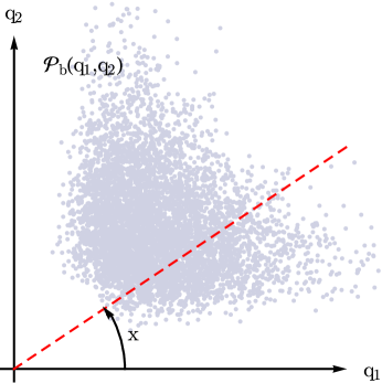
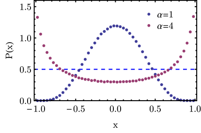
Figure 1: Sample pair distribution generated by chirality components of the lowest eigenmodes of ensemble $E_{1}$ from [2]. Right: the associated X-distribution, i.e., the induced distribution of the polarization angle.

The raw distribution ${\cal P}_{b}(q_{1},q_{2})$ is difficult to characterize. A more direct measure is offered by the induced distribution of the polarization angle. In Fig. 1 we plot the raw distribution of chirality components as determined in a previous study [2] and the corresponding polarization angle distribution (the curve indicated by $\alpha=1$), which we call the X-distribution. We see that the X-distribution tends to be concentrated towards the middle of the graph, suggesting an anti-polarization tendency.

A more careful analysis reveals that the conclusions based on this method can be misleading. The X-distribution is determined by the choice of parametrization for the angles measured in the $q_{1}q_{2}$-plane. The definition we used to plot Fig. 1 is

$$x=\frac{4}{\pi}\arctan\frac{\|Q_{2}\|}{\|Q_{1}\|}-1\,.$$ (3)

We will refer to this choice as the reference polarization [4]. However, this choice is not unique. Alternative definitions were used in various studies. Using $t\equiv{\|Q_{2}\|}/{\|Q_{1}\|}$, one class of valid angle variables is given by a generalization of the above definition

$$\bar{x}=\frac{4}{\pi}\arctan(t^{\alpha})-1\,,$$ (4)

where $\alpha>0$ is an arbitrary parameter [2]. For $\alpha=1$ the angle parameter $\bar{x}$ is the reference polarization defined above, while the definition based on $\bar{x}$ with $\alpha=2$ was used in a study of self-duality in pure gauge QCD [5]. In the right panel of Fig. 1 we compare the X-distribution for the ensemble shown in the left panel, measured using the reference polarization and the polarization defined by $\bar{x}$ with $\alpha=4$. The qualitative behavior of the distribution changes dramatically, while the dynamics producing the original distribution is unchanged. It is clear then that conclusions based on X-distributions alone cannot be trusted.

To address this problem we define the absolute X-distribution, a measure of the pair correlation induced by the underlying dynamics [2, 6]. The basic idea is to compare the correlated distribution ${\cal P}_{b}(q_{1},q_{2})$ with a similar distribution where the components are statistically independent, to isolate the effect of the dynamics. The uncorrelated distribution is constructed from the marginal distributions

$$P_{1}(q_{1})=\int dq_{2}\,{\cal P}_{b}(q_{1},q_{2})\qquad\text{and}\qquad P_{2}(q_{2})=\int dq_{1}\,{\cal P}_{b}(q_{1},q_{2})\,.$$ (5)

For our application, symmetry guarantees that $P_{1}=P_{2}$. The uncorrelated distribution is ${\cal P}_{u}(q_{1},q_{2})\equiv P_{1}(q_{1})P_{2}(q_{2})$. We define an angle variable that has constant angular density for the uncorrelated distribution. This is the absolute polarization. The histogram of this angle variable for the uncorrelated distribution is flat. In our figures this is indicated by a horizontal dashed line. The X-distribution in terms of the absolute polarization is the absolute X-distribution.

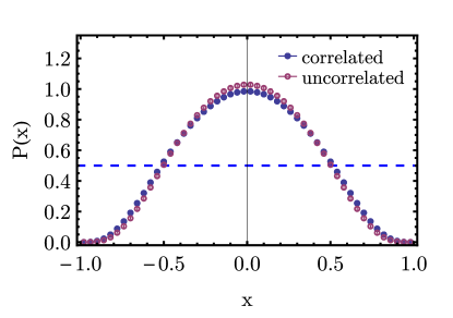
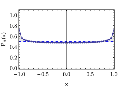
Figure 2: X-distribution using the reference polarization for the correlated and uncorrelated distributions (left) and the absolute X-distribution (right).

In the left panel of Fig. 2 we present the X-distribution for the reference polarizations for both correlated distribution, ${\cal P}_{b}$, and the uncorrelated one, ${\cal P}_{u}$, for the ensemble presented in Fig. 1. Notice that these two distributions are almost identical indicating that there is little dynamical correlation. In the right panel we plot the absolute polarization histogram, which is almost flat. There is a small enhancement towards the edges indicating that the dynamics induces a slight polarization. This is consistent with the plots in the right panel, where we see that the uncorrelated distribution is more prominent towards the center of the histogram.

Based on the absolute polarization distribution, $P_{A}(x)$, we construct a more compact measure of the polarization tendency, the correlation coefficient

$$C_{A}=2\Gamma-1\qquad\text{where}\qquad\Gamma=\int\limits_{-1}^{1}\!dx\,P_{A}(x)\left|x\right|\,.$$ (6)

The coefficient $\Gamma$ measures the probability that a sample drawn from distribution ${\cal P}_{b}$ is more polarized than one drawn from ${\cal P}_{u}$. When we have no dynamical correlation this probability is $0.5$; the correlation coefficient is scaled such that $C_{A}=0$ in this case.

3 Field strength definition

In this study, we will use a definition of the field strength based on the overlap operator. Compared to the ultra-local definitions, the overlap definition is less susceptible to ultra-violet fluctuations, so no arbitrary link smearing or cooling is needed. Moreover, this definition provides a natural expansion in terms of eigenmodes of the Dirac operator which allows us to define a smoothed version of field strength tensor controlled by the value of the eigenvalue cutoff.

If we denote with $S_{F}=\bar{\psi}D(x,y)\psi$ the fermionic contribution to the action in the overlap formulation, it is easy to show that $\mathop{\hbox{tr}}\nolimits_{s}\sigma_{\mu\nu}D(x,x)$ has the same quantum numbers as the field strength $F_{\mu\nu}$ [7]. Here $\mathop{\hbox{tr}}\nolimits_{s}$ denotes the trace over the spinor index. It was shown by explicit calculation that on smooth fields in the limit $a\to 0$ these definitions agree [8, 9],

$$\mathop{\hbox{tr}}\nolimits\nolimits_{s}\sigma_{\mu\nu}D(x,x)=c^{T}F_{\mu\nu}(x)+{\cal O}(a^{4})\,.$$ (7)

Above, $c^{T}$ is a constant that depends on the kernel used to define the overlap operator. The lattice version of the field strength operator used in this study is

$$F^{\text{ov}}_{\mu\nu}(x)\equiv\frac{1}{c^{T}}\mathop{\hbox{tr}}\nolimits_{s}\sigma_{\mu\nu}D(x,x)=-\frac{1}{c^{T}}\mathop{\hbox{tr}}\nolimits_{s}\sigma_{\mu\nu}[2\rho-D(x,x)]\,,$$ (8)

where $2\rho$ is the largest eigenvalue of $D$, the eigenvalue associated with the zero modes’ partners. We used the fact that $\mathop{\hbox{tr}}\nolimits_{s}\sigma_{\mu\nu}=0$ to cast the definition in a form useful for eigenmode expansion.

Using the expansion in terms of the eigenmodes of the Dirac operator, we define the smoothed version of the field strength [2]

$$F^{\Lambda}_{\mu\nu}(x)\equiv-\frac{1}{c^{T}}\sum_{|\lambda|<\Lambda a}\mathop{\hbox{tr}}\nolimits_{s}\sigma_{\mu\nu}(2\rho-\lambda)\psi_{\lambda}(x)\psi_{\lambda}(x)^{\dagger}\,.$$ (9)

This definition has the property that $\lim_{\Lambda\to\infty}F^{\Lambda}=F$ and that the contribution of the largest eigenmodes is suppressed. The self-dual and anti-self-dual parts of the field strength are defined using the dual of the field strength $\tilde{F}_{\mu,\nu}=\frac{1}{2}\epsilon_{\mu\nu\alpha\beta}F_{\alpha\beta}$

$$F_{S}=\frac{1}{2}(F+\tilde{F})\qquad F_{A}=\frac{1}{2}(F-\tilde{F})\,.$$ (10)

4 Numerical results

For our study we used a set of pure-glue ensembles generated using Iwasaki action [10]. The parameters for these ensembles are presented in Table 1. To study the continuum limit we have a set of 5 ensembles with the same volume. To determine the finite volume effects we also generated one ensemble with a larger volume.

Ensemble	Size	Lattice spacing	Volume	Configurations
$E_{2}$	$12^{4}$	$0.110\mathop{\hbox{fm}}$		400
$E_{3}$	$16^{4}$	$0.083\mathop{\hbox{fm}}$		200
$E_{8}$	$20^{4}$	$0.066\mathop{\hbox{fm}}$	$(1.32\mathop{\hbox{fm}})^{4}$	80
$E_{4}$	$24^{4}$	$0.055\mathop{\hbox{fm}}$		40
$E_{7}$	$32^{4}$	$0.041\mathop{\hbox{fm}}$		20
$E_{6}$	$32^{4}$	$0.055\mathop{\hbox{fm}}$	$(1.76\mathop{\hbox{fm}})^{4}$	20

Table 1: The size and lattice spacing for the ensembles used in this study.

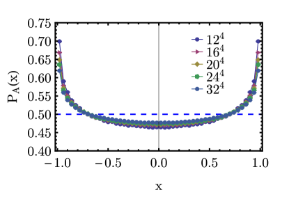
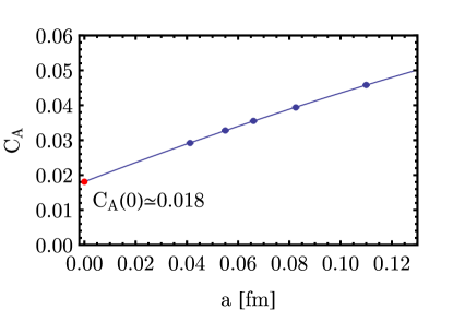
Figure 3: Left: absolute X-distribution for self-duality components. Note that the y-scale is magnified to better show the difference between different lattice spacings. Right: the correlation coefficient as a function of the lattice spacing and its continuum limit extrapolation. Error bars are present in these plots but they are smaller than the symbol size.

In Fig. 3 we plot the histogram for the absolute polarization for all ensembles with volume $(1.32\mathop{\hbox{fm}})^{4}$. We find a small tendency for polarization that decreases as we make the lattice spacing smaller. To understand whether this tendency survives the continuum limit, we compute the correlation coefficient and fit it with a quadratic polynomial in $a$. As we can see from the right panel of Fig. 3 the polynomial fits the data well. The coefficient remains positive in the continuum limit, indicating a very small tendency for polarization. The probability that the sample drawn from the correlated distribution is more polarized than one drawn from the uncorrelated distribution is 51% compared to 50% when the dynamics would produce no correlation.

To gauge the size of the finite volume effects, we compute the absolute polarization on two ensembles with the same lattice spacings but different volumes. Referring to Table 1, these are ensembles $E_{4}$ and $E_{6}$. In the left panel of Fig. 4 we compare the absolute polarizations on these two ensembles. We find no difference between the two histograms and we conclude that the finite volume effects are negligible.

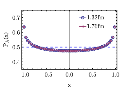
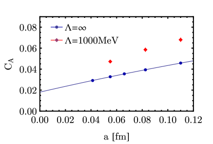
Figure 4: Left: absolute X-distribution for ensemble $E_{4}$ (circles) and $E_{6}$ (crosses) which have the same lattice spacing but different volume. Right: correlation coefficient for the smoothed strength field (diamonds) compared to the full version (circles). Error bars are included in both plots.

We also computed a set of eigenmodes of the overlap Dirac operators on ensembles $E_{2}$, $E_{3}$ and $E_{4}$ and used them to compute the smoothed field strength operator $F^{\Lambda}$. To study the continuum limit, a consistent definition of the smoothed operator sums over all modes smaller than a physical cutoff. We set the cutoff $\Lambda=1000\mathop{\hbox{MeV}}$ and found that the behavior of the absolute X-distribution is similar to the full version of the operator. In the right panel of Fig. 4 we compare the correlation coefficient with the one computed using the full operator. We find that while the values of the correlation coefficient are slightly different, the qualitative behavior remains the same.

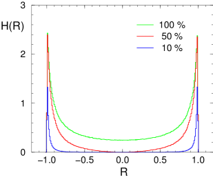
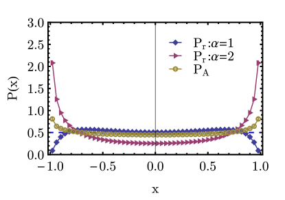
Figure 5: Left: X-distribution for self-duality components of a smooth field strength based on the low-lying modes of the chirally-improved Dirac operator [5]. The curved marked with 100% is the relevant one for our comparison. Right: absolute X-distribution $P_{A}$ and X-distribution $P_{r}$ based on two different polarization variables (see Eq. 4) for ensemble $E_{2}$.

We conclude our discussion with a comparison with a similar work by Gattringer [5] who studied the self-duality polarization using a smoothed field strength operator. This operator was constructed using an eigenmode expansion of the chirally-improved Dirac operator. In Ref. [5] it was found that the self-duality exhibits a strong polarization (see left panel of Fig. 5) supporting a model of vacuum dominated by topological “lumps”. In contrast, we only find a mild dynamical tendency for polarization. This is seen in the right panel of Fig. 5 where we plot the absolute X-distribution of ensemble $E_{2}$ which is similar to the ensemble used in Ref. [5]. The discrepancy is due to the fact that Ref. [5] uses a polarization measure dominated by kinematical effects. To show this, in the right panel of Fig. 5 we also plot the X-distribution measured using the reference polarization, $\alpha=1$, and the polarization angle used in Ref. [5], $\alpha=2$. To better compare our results, for these plots we used, as in the referenced study, a smoothed $F^{\Lambda}$ constructed using the same number of modes. We see then that when using the same angle definition, our results are consistent with those of Ref. [5]. However, using another valid angle parametrization produces qualitatively different results due to kinematical effects. We conclude that the strong polarization observed in Ref. [5] is mainly due to the specific choice of angle variable rather than the underlying dynamics.

5 Conclusions

In this work we studied the dynamical polarization propertied of self-duality components induced by pure-glue QCD dynamics. We found a very mild polarization tendency that survives in the continuum limit. This results has negligible finite-volume corrections. The self-duality tendency is very small making it unlikely that the vacuum fluctuations are well-described by semi-classical models. Our findings are at variance with the results of a previous study [5]. We conclude that the discrepancy is the result of kinematical effects.

Acknowledgments: Andrei Alexandru is supported in part under DOE grant DE-FG02-95ER-40907. The computational resources for this project were provided in part by the George Washington University IMPACT initiative. Ivan Horváth acknowledges warm hospitality of the BNL Theory Group during which part of this work has been completed.

References

- [1] T. Schafer and E. V. Shuryak, Instantons in QCD, Rev.Mod.Phys. 70 (1998) 323–426, [hep-ph/9610451].
- [2] A. Alexandru, T. Draper, I. Horváth, and T. Streuer, The Analysis of Space-Time Structure in QCD Vacuum II: Dynamics of Polarization and Absolute X-Distribution, Annals of Physics 326 (2011) 1941–1971, [arXiv:1009.4451].
- [3] A. Alexandru and I. Horváth, How Self-Dual is QCD?, arXiv:1110.2762.
- [4] I. Horváth, N. Isgur, J. McCune, and H. B. Thacker, Evidence against instanton dominance of topological charge fluctuations in QCD, Phys. Rev. D65 (2002) 014502, [hep-lat/0102003].
- [5] C. Gattringer, Testing the self-duality of topological lumps in SU(3) lattice gauge theory, Phys. Rev. Lett. 88 (2002) 221601, [hep-lat/0202002].
- [6] T. Draper, A. Alexandru, Y. Chen, S.-J. Dong, I. Horváth, et. al., Improved measure of local chirality, Nucl.Phys.Proc.Suppl. 140 (2005) 623–625, [hep-lat/0408006].
- [7] I. Horváth, A Framework for Systematic Study of QCD Vacuum Structure II: Coherent Lattice QCD, hep-lat/0607031.
- [8] K. Liu, A. Alexandru, and I. Horváth, Gauge field strength tensor from the overlap Dirac operator, Phys.Lett. B659 (2008) 773–782, [hep-lat/0703010].
- [9] A. Alexandru, I. Horváth, and K.-F. Liu, Classical Limits of Scalar and Tensor Gauge Operators Based on the Overlap Dirac Matrix, Phys.Rev. D78 (2008) 085002, [arXiv:0803.2744].
- [10] CP-PACS Collaboration Collaboration, M. Okamoto et. al., Equation of state for pure SU(3) gauge theory with renormalization group improved action, Phys.Rev. D60 (1999) 094510, [hep-lat/9905005].