Effects of a spin-flavour dependent interaction on the baryon mass spectrum

Abstract

The effective quark interaction in a relativistically covariant constituent quark model based on the Salpeter equation is supplemented by an extra phenomenological flavour dependent force in order to account for some discrepancies mainly in the description of excited negative parity $\Delta$ resonances. Simultaneously an improved description of some other features of the light-flavoured baryon mass spectrum and of some electromagnetic form factors is obtained.

1 Introduction

The description of the hadronic excitation spectrum remains a major challenge in strong interaction theory. In spite of recent progress in unquenched lattice QCD access to excited states is still very limited Edwards ; Huey-Wen . Therefore it seems worthwhile to improve upon constituent quark model descriptions, which in view of the light quarkmasses (even taken as effective constituent masses) have to be formulated in terms of relativistically covariant equations of motion. About a decade ago we formulated such a quark model for baryons, see LoeMePe1 ; LoeMePe2 ; LoeMePe3 on the basis of an instantaneous formulation of the Bethe-Salpeter equation. In this model the quark interactions reflect a string-like description of quark confinement through a confinement potential rising linearly with interquark distances as well as a spin-flavour dependent interaction on the basis of instanton effects, which explains the major spin-dependent splittings in the baryon spectrum.

Such a model description should offer an efficient description of masses (resonance positions), static properties such as magnetic moments, charge radii, electroweak amplitudes (form factors and helicity amplitudes) with only a few model parameters. As such they also offer a framework which can be used to judge in how far certain features could be considered to be exotic. This concerns e.g. phenomenological evidence for states with properties that can not be accounted for in terms of excitations of quark degrees of freedom, as is at the heart of any constituent quark model, but instead requires additional degrees of freedom as e.g. reflected by hadronic interactions.

A satisfactory description of the major features in the light-flavoured baryonic mass spectrum could indeed be obtained. These include

• the linear Regge trajectories with an universal slope for all flavours including states up to total angular momenta of $J=\frac{15}{2}$ and excitation energies up to 3 GeV, see LoeMePe2 ; LoeMePe3 ;

• the position of the Roper-resonance and three other positive parity excited nucleon states well below all other states of this kind. These can be largely accounted for by the instanton-induced force, thestrength of which was chosen to reproduce the ground state $N-\Delta$ splitting LoeMePe2 ; LoeMePe3 ;

• a plethora of electroweak properties which can be explained without introducing any additional parameters, see Merten ; vCauteren ; Haupt .

Nevertheless some specific discrepancies remain; most prominent are:

• the conspicuously low position as well as the decay properties of the negative parity $\Lambda_{\frac{1}{2}^{-}}(1405)$ resonance; The calculated mass of this state exceeds the experimental value by more than 100 MeV;

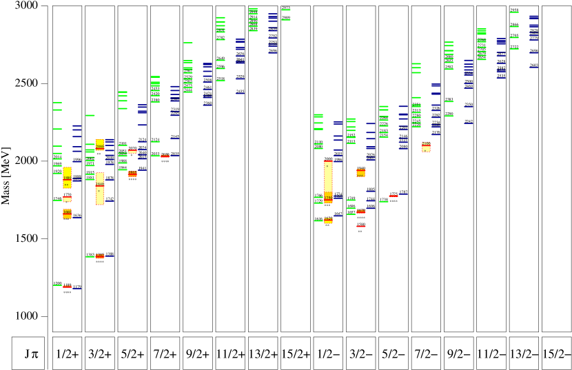
• there is experimental evidence PDG for excited negative parity $\Delta$-resonances well below 2 GeV which can not be accounted for by the quark model mentioned above, see fig. 1,

  

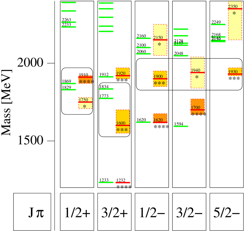
  Fig. 1: Discrepancies in the $\Delta$ mass spectrum: The left part of each column represents the results obtained in model $\mathcal{A}$ of LoeMePe2 in comparison with experimental data from the Particle Data Group PDG (right side of each column), where lines are the resonance position (mass) with the mass uncertainty represented by a shaded box and the rating of PDG indicated by stars. $J$ and $\pi$ denote total angular momentum and parity, respectively. Small differences with respect to the results from fig. 3 of LoeMePe2 are due to the fact that we obtained increased numerical accuracy by diagonalising the resulting Salpeter Hamiltonian in larger model spaces, see section 2.2 for details.

  nor by any other constituent quark model we are aware of;

• The mass of the positive parity $\Delta_{\frac{3}{2}^{+}}(1600)$ resonance, see also fig. 1, the low value of which with respect to other excited states of this kind can not be traced back to instanton-induced effects, since these are absent for flavour symmetric states.

We therefore want to explore whether these deficiencies are inherent to the constituent quark model itself or can be overcome by the introduction of an additional quark interaction which improves upon the issues mentioned above without deteriorating the excellent description of the majority of the other states. In view of the fact that the discrepancies mainly affect the $\Delta$-spectrum, this additional interaction is likely to be flavour dependent. An obvious candidate in this respect would be a single pseudoscalar meson exchange potential as has been used as a basis of an effective spin-flavour dependent quark interaction very successfully by the Graz-group Glozman1996 ; Glozman1997 ; Glozman1998_1 ; Glozman1998_2 ; Theussl ; Glantschnig ; Melde08 ; Plessas .

In the present paper we shall investigate various implementations of the coordinate (or momentum) dependence of such interactions. The paper is organised as follows: After a brief recapitulation of the ingredients and basic equations of our Bethe-Salpeter model (for more details see LoeMePe1 ) in section 2, we discuss in section 3 the form and the parameters of the effective quark interactions used in this paper. Section 4 contains the results and a discussion of the baryon mass spectra in comparison to the results obtained before LoeMePe2 ; LoeMePe3 . In section 5 we present some results on ground state form factors before concluding in section 6.

2 Bethe-Salpeter model

2.1 Bound state Bethe-Salpeter amplitudes

The basic quantity describing three-quark bound states is the Bethe-Salpeter amplitude $\chi$ defined in position space through

$$\chi_{\bar{P}\,a_{1}a_{2}a_{3}}(x_{1},x_{2},x_{3})$$ (1)

$$=\langle 0|T\,\Psi_{a_{1}}(x_{1})\Psi_{a_{2}}(x_{2})\Psi_{a_{3}}(x_{3})|\bar{P}\rangle\,,$$

where $T$ is the time ordering operator, $\left|\bar{P}\right\rangle$ represents the bound-state with total 4 momentum $\bar{P}^{2}=M^{2}$ of a baryon with mass $M$ , $\left|0\right\rangle$ is the physical vacuum and $\Psi_{a_{i}}(x_{i})$ denotes single quark-field operators with multi-indices $a_{i}$ in Dirac, colour and flavour space. Because of translational invariance below we shall exclusively use relative Jacobi coordinates $p_{\xi},p_{\eta}$ in momentum space. The Fourier transform of the Bethe-Salpeter amplitudes: $\chi_{\bar{P}\,a_{1}a_{2}a_{3}}(p_{\xi},p_{\eta})$ are then determined by the homogeneous
Bethe-Salpeter equation compactly written as

$$\chi_{\bar{P}}=-\textrm{i}\,G_{0\,,P}\left(K^{(3)}_{\bar{P}}+\bar{K}^{(2)}_{\bar{P}}\right)\,\chi_{\bar{P}}\,,$$ (2)

where $K^{(3)}_{P}$ represents the irreducible 3-quark-kernel and where $\bar{K}^{(2)}_{P}$ is defined by

$$\bar{K}^{(2)}_{P}(p_{\xi},p_{\eta};p_{\xi}^{\prime},p_{\eta}^{\prime})=\sum_{k=1}^{3}(2\pi)^{4}\,\delta^{(4)}(p_{\eta_{k}}-p_{\eta_{k}}^{\prime})\,$$ (3)

$$\times K^{(2)}_{(\frac{2}{3}P+p_{\eta_{k}})}(p_{\xi_{k}},p_{\xi_{k}}^{\prime})\otimes\left(S_{F}^{3}\right)^{-1}\!\!\left(\textstyle\frac{P}{3}-p_{\eta_{k}}\right)$$

in terms of the irreducible two-body interaction kernel
$K^{(2)}_{\!(\!\frac{2}{3}P+p_{\eta_{k}}\!)}$ for each quark pair labeled by the odd-particle index $k$. Furthermore $G_{0,P}$ is the free 3-quark fermion propagator defined as

$$G_{0,P}(p_{\xi},p_{\eta};p_{\xi}^{\prime},p_{\eta}^{\prime})=$$ (4)

$$(2\pi)^{8}\,\delta^{(4)}(p_{\xi}-p_{\xi}^{\prime})\,\delta^{(4)}(p_{\eta}-p_{\eta}^{\prime})$$

$$\times S^{1}_{F}(\textstyle\frac{P}{3}\!+\!p_{\xi}\!+\!\frac{p_{\eta}}{2})\!\otimes\!S^{2}_{F}(\frac{P}{3}\!-\!p_{\xi}\!+\!\frac{p_{\eta}}{2})\!\otimes\!S^{3}_{F}(\frac{P}{3}\!-\!p_{\eta})$$

in terms of full single quark propagators $S^{i}_{F}$ .

2.2 Model assumptions

In view of the fact that the interaction kernels and the propagators are sums of infinitely many Feynman diagrams, in order to arrive at a tractable model we make the following assumptions, mainly with the goal to stay in close contact with the quite successful non-relativistic constituent quark model:

• The full propagators $S^{i}_{F}$ are replaced by Feynman propagators of the free form

  $$S^{i}_{F}(p)\overset{!}{=}\frac{\textrm{i}}{p\!\!\!/-m_{i}+\textrm{i}\,\varepsilon}\,,$$ (5)

  tacitly assuming that at least some part of the self-energy can effectively be subsumed in an effective constituent quark mass $m_{i}$ which then is a parameter of the model.

• Obviously this does not account for confinement: This is assumed to be implemented in the form of an instantaneous interaction kernel which in the rest frame of the baryon is described by an unretarded potential $V^{(3)}$ :

  $$K^{(3)}_{P}\left(p_{\xi},p_{\eta};{p_{\xi}}^{\prime},{p_{\eta}}^{\prime}\right) \Big{|}_{P=(M,\vec{0})}$$

  $$\overset{!}{=}\, V^{(3)}\left(\vec{p}_{\xi},\vec{p}_{\eta};{\vec{p}_{\xi}}^{\prime},{\vec{p}_{\eta}}^{\prime}\right)\,.$$ (6)

  Likewise we assume that two-quark interaction kernels in the rest frame of the baryon are described by 2-body potentials $V^{(2)}$ :

  $$K^{(2)}_{\frac{2}{3}P+p_{\eta_{k}}}\left(p_{\xi_{k}};{p_{\xi_{k}}}^{\prime}\right) \Big{|}_{P=(M,\vec{0})}$$

  $$\overset{!}{=}\, V^{(2)}\left(\vec{p}_{\xi_{k}};{\vec{p}_{\xi_{k}}}^{\prime}\right)\,.$$ (7)

Then, with a perturbative elimination of retardation effects, which arise due to the genuine two-body interactions, see  LoeMePe1 for details, one can derive an equation for the (projected) Salpeter amplitude

$$\Phi^{\Lambda}_{M}(\vec{p}_{\xi},\vec{p}_{\eta})=\Lambda_{+}(\vec{p}_{\xi},p_{\eta})\int\frac{\textrm{d}p^{0}_{\xi}}{2\pi}\frac{\textrm{d}p^{0}_{\eta}}{2\pi}\chi_{M}(p_{\xi},p_{\eta})\,,$$ (8)

where

$$\Lambda_{\pm}(\vec{p}_{\xi},p_{\eta}):=\Lambda^{+}(\vec{p}_{1})\otimes\Lambda^{+}(\vec{p}_{2})\otimes\Lambda^{+}(\vec{p}_{3})$$

$$\pm\,\,\Lambda^{-}(\vec{p}_{1})\otimes\Lambda^{-}(\vec{p}_{2})\otimes\Lambda^{-}(\vec{p}_{3})$$ (9)

with

$$\Lambda^{\pm}(\vec{p})=\sum_{f}\Lambda^{\pm}_{m_{f}}(\vec{p})\otimes\mathcal{P}_{f}\,.$$ (10)

Here

$$\Lambda^{\pm}_{m}(\vec{p}):=\frac{\omega_{m}(\vec{p})\pm H_{m}(\vec{p})}{2\,\omega_{m}(\vec{p})}$$ (11)

are projection operators on positive and negative energy states and $\mathcal{P}_{f}$ projects on quark flavour $f$ . Furthermore the quark energy is given by $\omega(\vec{p})=\sqrt{|\vec{p}|^{2}+m^{2}}$ and

$$H_{m}(\vec{p}):=\gamma^{0}\left(\vec{\gamma}\cdot\vec{p}+m\right)$$ (12)

is the Dirac Hamilton operator. As shown in detail in LoeMePe1 this equation can be written in the form of an eigenvalue problem

$$\mathcal{H}\,\Phi^{\Lambda}_{M}=M\,\Phi^{\Lambda}_{m}$$ (13)

for the projected Salpeter amplitude, where the eigenvalues are the baryon masses $M$ . The Salpeter Hamilton operator is given by

$$\left[\mathcal{H}\,\Phi^{\Lambda}_{M}\right](\vec{p}_{\xi},\vec{p}_{\eta})=\mathcal{H}_{0}(\vec{p}_{\xi},\vec{p}_{\eta})\,\Phi^{\Lambda}_{M}(\vec{p}_{\xi},\vec{p}_{\eta})$$

$$+ \Lambda_{+}(\vec{p}_{\xi},\vec{p}_{\eta})\,\gamma^{0}\!\otimes\!\gamma^{0}\!\otimes\!\gamma^{0}\!\otimes\!\int\frac{\textrm{d}^{3}{p_{\xi}}^{\prime}}{(2\pi)^{3}}\frac{\textrm{d}^{3}{p_{\eta}}^{\prime}}{(2\pi)^{3}}$$

$$\hskip 30.00005ptV^{(3)}(\vec{p}_{\xi},\vec{p}_{\eta};{\vec{p}_{\xi}}^{\prime},{\vec{p}_{\eta}}^{\prime})\,\Phi^{\Lambda}_{M}({\vec{p}_{\xi}}^{\prime},{\vec{p}_{\eta}}^{\prime})$$

$$+ \Lambda_{-}(\vec{p}_{\xi},\vec{p}_{\eta})\,\gamma^{0}\!\otimes\!\gamma^{0}\!\otimes\!\mathds{1}\int\frac{\textrm{d}^{3}{p_{\xi}}^{\prime}}{(2\pi)^{3}}$$

$$\hskip 30.00005pt\,V^{(2)}(\vec{p}_{\xi};{\vec{p}_{\xi}}^{\prime})\otimes\!\mathds{1}\,\Phi^{\Lambda}_{M}({\vec{p}_{\xi}}^{\prime},{\vec{p}_{\eta}})$$

$$+ \textrm{corresponding quark interations (23) and (31)}\,,$$

where $\mathcal{H}_{0}$ denotes the free three-quark Hamilton operator as a sum of the corresponding single particle Dirac Hamilton operators.

The eigenvalue problem of Eq. (13) is solved by numerical diagonalisation in a large but finite basis of oscillator states up to an oscillator quantum number $N_{\textrm{max}}$ . In previous calculations LoeMePe2 ; LoeMePe3 at least $N_{\textrm{max}}=12$ was used. All the results in the present paper were obtained with at least $N_{\textrm{max}}=18$ , which, although computer time consuming, has the advantage that for all states the independence of the numerical results on the oscillator functions length scale in some scaling window could be warranted and that all could be calculated with a universal value for this length scale. This is a technical advantage when calculating electroweak amplitudes.

3 Model Interactions

Below we specify the interaction potentials $V^{(3)}$ and $V^{(2)}$ used in Eq. (2.2) . These include a confinement potential, the instanton induced two-quark interaction as has been used before LoeMePe2 ; LoeMePe3 and the new phenomenological potential inspired by pseudoscalar meson exchange.

3.1 Confinement

Confinement is implemented by subjecting the quarks to a potential which rises linearly with interquark distances, supplemented by an appropriate three particle Diracstructure $\Gamma$. The potential contains two parameters: the off-set $a$ and the slope $b$ and is assumed to be of the following form in coordinate space

$$V^{(3)}_{\textrm{conf}}(\vec{x}_{1},\vec{x}_{2},\vec{x}_{3})\,=3\,a\,\Gamma_{o}+b\sum_{i<j}\left|\vec{x}_{i}-\vec{x}_{j}\right|\,\Gamma_{s}$$ (15)

where $\Gamma_{o}$ and $\Gamma_{s}$ are suitably chosen Dirac structures. Alternatively we can consider the linear potential to be treated as a two-body kernel as will be used below.

3.2 Instanton induced interaction

Instanton effects leads to an effective quark-quark interaction, which for quark pairs in baryons can be written in coordinate space as

$$\mathcal{V}^{(2)}_{\textrm{III}}(x_{1},x_{2};x_{1}^{\prime}x_{2}^{\prime})=V^{(2)}_{\textrm{III}}(\vec{x}_{1}-\vec{x}_{2})$$ (16)

$$\hskip 25.00003pt\times\,\delta(x_{1}^{0}-x_{2}^{0})\,\delta^{(4)}(x_{1}-x_{1}^{\prime})\,\delta^{(4)}(x_{2}-x_{2}^{\prime})$$

with

$$V^{(2)}_{\textrm{III}}(\vec{x})\, = -4v(\vec{x})\left(\mathds{1}\!\otimes\!\mathds{1}+\gamma^{5}\!\otimes\!\gamma^{5}\right)\mathcal{P}^{\mathcal{D}}_{S_{12}=0}$$ (17)

$$\!\otimes\!\left(g_{nn}\,\mathcal{P}^{\mathcal{F}}_{\mathcal{A}}(nn)+g_{ns}\,\mathcal{P}^{\mathcal{F}}_{\mathcal{A}}(ns)\right)\,,$$

where $\mathcal{P}^{\mathcal{D}}_{S_{12}=0}$ is a projector on spin-singlet states and $\mathcal{P}^{\mathcal{F}}_{\mathcal{A}}(f_{1}f_{2})$ projects on flavour-antisymmetric quark pairs with flavours $f_{1}$ and $f_{2}$. Although the two couplings $g_{nn}$ and $g_{ns}$ are in principle determined by integrals over instanton densities, these are treated as free parameters here. As it stands this is a contact interaction, which for our purpose is regularised by replacing the coordinate space dependence by a Gaussian

$$v_{\lambda}(\vec{x})=\frac{1}{\lambda^{3}\,\pi^{\frac{3}{2}}}\,\exp\left(-\tfrac{|\vec{x}|^{2}}{\lambda^{2}}\right)\,.$$ (18)

The effective range parameter $\lambda$ is assumed to be flavour independent and enters as an additional parameter.

3.3 An additional flavour dependent interaction

The coupling of spin-$\frac{1}{2}$ fermions to a flavour nonet of pseudoscalar meson fields is given by an interaction Lagrange density

$$\mathcal{L}_{I}^{\textnormal{(ps)}}=-\mathrm{i}\sum_{a=0}^{8}g_{a}\,\bar{\psi}\,\gamma^{5}\,\lambda^{a}\,\psi\,\phi^{a},$$ (19)

in the case of so-called pseudoscalar coupling and by

$$\mathcal{L}_{I}^{\textnormal{(pv)}}=-\sum_{a=0}^{8}\frac{g_{a}}{2m}\,\bar{\psi}\,\gamma^{5}\,\gamma^{\mu}\,\lambda^{a}\,\psi\,\partial_{\mu}\phi^{a}.$$ (20)

for pseudovector coupling. Here $\psi$ represents the quark fields with mass $m$ and $\phi^{a}$ the pseudoscalar meson fields with mass $\mu_{a}$ where the flavour index $a=\pi^{\pm\,,0},\eta^{0}_{8},$ $\eta_{1}^{0}$ $K^{\pm},$ $K^{0},$ $\bar{K}^{0}$ . The flavour dependence is represented by the usual Gell-Mann matrices $\lambda^{a},a=1,\ldots,8$ ; $\lambda^{0}$ is proportional to the identity operator in flavour space normalised to $\textrm{Tr}((\lambda^{0})^{2})=2$.

A standard application of the Feynman rules, see e.g.  CaDuElHaSiSp then leads to the second order scattering-matrix element $\mathcal{M}^{(2)}$ given in the CM-system by the expressions

$$\mathrm{i}\mathcal{M}_{\textnormal{(ps)}}^{(2)}(k_{0},\vec{k})$$ (21)

$$= \sum_{a,b}g_{a}^{2}\bigg{[}\bar{\psi}(\vec{p}^{\prime})(-i\gamma^{5})\lambda^{a}\,\psi(\vec{p})\,D^{ab}(k_{0},\vec{k})$$

$$\hskip 10.00002pt\times\bar{\psi}(-\vec{p}^{\prime})(-\mathrm{i}\gamma^{5})\lambda^{b}\psi(-\vec{p})\bigg{]}$$

$$=: -\sum_{a,b}g_{a}^{2}D^{ab}(k_{0},\vec{k})\left[\lambda^{a}\,\gamma^{5}\right]\!\otimes\!\left[\lambda^{b}\,\gamma^{5}\right]$$

$$=: \mathrm{i}[\bar{\psi}(-\vec{p}^{\prime})\!\otimes\!\bar{\psi}(\vec{p}^{\prime})]V_{(ps)}(k_{0},\vec{k})[\psi(-\vec{p})\!\otimes\!\psi(\vec{p})]$$

and

$$\mathrm{i}\,\mathcal{M}_{\textnormal{(pv)}}^{(2)}(k_{0},\vec{k})$$ (22)

$$= \sum_{a,b}\frac{g_{a}^{2}}{4m^{2}}\bigg{[}\bar{\psi}(\vec{p}^{\prime})\gamma^{5}\gamma^{\mu}(-ik_{\mu})\lambda_{a}\psi(\vec{p})\,D^{ab}(k_{0},\vec{k})$$

$$\hskip 10.00002pt\times\bar{\psi}(-\vec{p}^{\prime})\gamma^{5}\gamma^{\nu}(-i(-k_{\nu}))\lambda_{b}\psi(-\vec{p})\bigg{]}$$

$$=: \sum_{a,b}\frac{g_{a}^{2}}{4m^{2}}\,D^{ab}(k_{0},\vec{k})\,k_{\mu}k_{\nu}\!\left[\lambda^{a}\gamma^{5}\gamma^{\mu}\right]\!\!\otimes\!\!\left[\lambda^{b}\gamma^{5}\gamma^{\nu}\right]$$

$$:= \mathrm{i}\,[\bar{\psi}(-\vec{p}^{\prime})\!\otimes\!\bar{\psi}(\vec{p}^{\prime})]V_{(pv)}(k_{0},\vec{k})[\psi(-\vec{p})\!\otimes\!\psi(\vec{p})]$$

in case of pseudoscalar and pseudovector coupling, respectively. Here the meson propagator is given by

$$D^{ab}(k_{0},\vec{k})=\frac{\mathrm{i}\delta_{ab}}{k_{0}^{2}-|\vec{k}|^{2}-\mu_{a}^{2}}\,,$$ (23)

with $k_{\mu}:=p_{\mu}^{\prime}-p_{\mu}$ the momentum transfer.

In instantaneous approximation we set $k_{0}=0$. From Eqs. [21,22] we extract the corresponding potentials in momentum space

$$V_{(ps)}^{(2)}(\vec{k})=\sum_{a}g_{a}^{2}[\lambda^{a}\!\otimes\!\lambda^{a}]\frac{1}{|\vec{k}|^{2}+\mu_{a}^{2}}\bigg{[}\gamma^{5}\!\otimes\!\gamma^{5}\bigg{]}$$ (24)

for pseudoscalar coupling and

$$V_{(pv)}^{(2)}(\vec{k})$$

$$= \sum_{a}\frac{g_{a}^{2}}{4m^{2}}[\lambda^{a}\!\otimes\!\lambda^{a}]\frac{-1}{|\vec{k}|^{2}+\mu_{a}^{2}}\Big{[}\!\big{(}\gamma^{5}\vec{\gamma}\cdot\vec{k}\big{)}\!\otimes\!\big{(}\gamma^{5}\bm{\gamma}\cdot\vec{k}\big{)}\!\Big{]}$$

$$= \sum_{a}\frac{g_{a}^{2}}{4m^{2}}[\lambda^{a}\!\otimes\!\lambda^{a}]\frac{-|\vec{k}|^{2}}{|\vec{k}|^{2}+\mu_{a}^{2}}\Big{[}\!\big{(}\gamma^{5}\vec{\gamma}\cdot\widehat{\vec{k}}\big{)}\!\otimes\!\big{(}\gamma^{5}\bm{\gamma}\cdot\widehat{\vec{k}}\big{)}\!\Big{]}$$

for pseudovector coupling, where $\widehat{\vec{k}}:=\frac{\vec{k}}{|\vec{k}|}$ .

As it stands, the expression for the potential in the instantaneous approximation for pseudoscalar coupling
leads, after Fourier transformation, to a local Yukawa potential in configuration space with the usual range given by the mass of the exchanged pseudoscalar meson. For pseudovector coupling the non-relativistic approximation to the Fourier transform leads to the usual spin-spin contact interaction together with the usual tensor force. In the simplest form adopted by the Graz group Glozman1996 ; Glozman1997 ; Glozman1998_1 ; Theussl ; Glantschnig ; Melde08 ; Plessas the latter were ignored, in addition the contact term was regularised by a Gaussian function and the Yukawa terms were regularised to avoid singularities at the origin.

In view of this and the instantaneous approximation we decided to parametrise the new flavour dependent interaction purely phenomenologically as a local potential in configuration space, its simple form given by

$$V^{(2)}(\vec{x})=\sum_{a}g_{a}^{2}\,\left[\lambda^{a}\,\gamma^{5}\!\otimes\!\lambda^{a}\,\gamma^{5}\right]\,v_{\lambda_{a}}(\vec{x})$$ (26)

where $v_{\lambda}(\vec{x})$ is the Gaussian form given in Eq. 18 . Other Dirac structures, such as $\left[\gamma^{5}\vec{\gamma}\cdot\widehat{\vec{x}}\,\!\otimes\!\gamma^{5}\vec{\gamma}\cdot\widehat{\vec{x}}\right]$ were tried, but were found to be less effective. Results for the meson exchange form of the interaction as given by Eqs. (24,3.3) will be briefly discussed in section 6.

Table 1: The list of baryon resonances of which the masses were used to determine the model parameters in a least-squares fit where every resonance was attributed a weight reciprocal to its uncertainty in its position as given in PDG . Nominal masses are given in MeV.

$\Delta$	$N$	$\Lambda/\Sigma$	$\Xi$	$\Omega$
$S_{31}(1620)$	$S_{11}(1535)$	$S_{21}(1620)$	$S_{11}(1309)$
$S_{31}(1900)$	$S_{11}(1650)$	$S_{21}(1750)$
$P_{31}(1750)$	$P_{11}(939)$	$P_{01}(1116)$	$P_{13}(1530)$	$P_{01}(1672)$
$P_{31}(1910)$	$P_{11}(1440)$	$P_{21}(1289)$
$P_{33}(1232)$		$P_{01}(1600)$
$P_{33}(1600)$		$P_{21}(1660)$
$P_{33}(1920)$
$D_{33}(1700)$			$D_{13}(1820)$
$D_{33}(1940)$
$D_{35}(1930)$
$F_{35}(1905)$
$F_{35}(2000)$
$F_{37}(1950)$
$G_{37}(2200)$
$G_{39}(2400)$
$H_{39}(2300)$
$H_{3\,11}(2420)\!\!\!$
$K_{3\,15}(2950)\!\!\!$

4 Mass spectra

4.1 Model parameters

The resulting baryon mass spectra were obtained by fitting the parameters of the model, viz. the offset $a$ and slope $b$ of the confinement potential, the constituent quark masses $m_{n}=m_{u}=m_{d}$ and $m_{s}$, the strengths of the instanton induced force, $g_{nn}$ and $g_{ns}$ as well as the strengths of the additional flavour dependent interaction, given by $g_{8}$ and $g_{0}$ for flavour octet and flavour singlet exchange (thus assuming $SU(3)$ symmetry) to a selection of baryon resonances, see table 1 . The range $\lambda$ given to the instanton induced force was kept to the value used in LoeMePe2 ; LoeMePe3 and is roughly in accordance with typical instanton sizes. The optimal value for the range of the additional flavour dependent interaction was found to be $\lambda_{8}=\lambda_{0}\approx 0.25\,\textnormal{fm}$ and thus turned out to be of rather short range. A comparison of the parameters obtained with the parameters of model $\mathcal{A}$ of LoeMePe2 ; LoeMePe3 is given in table 2 .

Table 2: Model parameters for the current model $\mathcal{C}$ in comparison to those of model $\mathcal{A}$ of LoeMePe2 ; LoeMePe3 . Some of the parameters have been slightly changed with respect to the original values (listed in brackets) of LoeMePe2 ; LoeMePe3 , since the calculation has been performed with higher numerical accuracy by taking more basis states in the diagonalisation of the Salpeter Hamiltonian, see also text.

parameter		model $\mathcal{C}$	model $\mathcal{A}$
masses	$m_{n}$ [MeV]	325.0	330.0
	$m_{s}$ [MeV]	600.0	670.0
confinement	$a$ [MeV]	-366.78	-734.6
			[-744.0]
	$b$ [MeV/fm]	212.81	453.6
			[440.0]
instanton	$g_{nn}$ [MeV fm3]	341.49	130.3
			[136.0]
induced	$g_{ns}$ [MeV fm3]	273.55	81.8
			[96.0]
interaction	$\lambda$ [fm]	0.4	0.4
octet	$\frac{g_{8}^{2}}{4\pi}$ [MeV fm3]	100.86	–
exchange
singlet	$\frac{g_{0}^{2}}{4\pi}$ [MeV fm3]	1897.43	–
exchange
	$\lambda_{8}=\lambda_{0}$ [fm]	0.25	–

Table 3: Multiplet decomposition of amplitudes of negative parity $\Delta$-resonances. For each amplitude the contribution to the Salpeter norm, see LoeMePe1 is given in $\%$ , in each row the upper line and the lower line give the positive and negative energy contribution, respectively. States are labeled by the calculated mass and $J^{\pi}$ denotes total angular momentum and parity, ${}^{2S+1}\mathcal{F}_{J}[D]$ label amplitudes with spin $S$, flavour representation with dimension $\mathcal{F}$, $SU(6)$ representation with dimension $D$ . The dominant contribution is underlined.

$J^{\pi}$	Mass	pos.	${}^{4}10_{J}[56]$	${}^{2}10_{J}[70]$
		neg.	${}^{4}10_{J}[56]$	${}^{2}10_{J}[70]$
$\frac{1}{2}^{-}$	1635	98.9	6.6	92.3
		1.1	0.8	0.4
$\frac{1}{2}^{-}$	1932	98.5	14.2	84.3
		1.5	1.0	0.5
$\frac{1}{2}^{-}$	2041	99.0	81.6	17.3
		1.0	0.5	0.5
$\frac{3}{2}^{-}$	1592	98.2	9.9	88.4
		1.8	0.9	0.9
$\frac{3}{2}^{-}$	1871	97.9	24.5	73.3
		2.1	1.4	0.7
$\frac{3}{2}^{-}$	1944	98.6	65.1	33.5
		1.4	0.9	0.6
$\frac{5}{2}^{-}$	2013	98.8	89.3	9.6
		1.2	0.6	0.6
$\frac{5}{2}^{-}$	2136	99.2	16.8	82.4
		0.8	0.3	0.5
$\frac{5}{2}^{-}$	2166	99.1	86.6	12.4
		1.0	0.4	0.6

The parameters need some comments: In the original paper LoeMePe2 ; LoeMePe3 the Dirac structures (i.e. the spin dependence) of the confinement potential were taken to be $\Gamma_{0}=\frac{1}{4}(\mathds{1}\!\otimes\!\mathds{1}\!\otimes\!\mathds{1}+\gamma^{0}\!\otimes\!\gamma^{0}\!\otimes\!\mathds{1}+\textrm{cycl. perm.})$ and $\Gamma_{s}=\frac{1}{2}(-\mathds{1}\!\otimes\!\mathds{1}\!\otimes\!\mathds{1}+\gamma^{0}\!\otimes\!\gamma^{0}\otimes\mathds{1}+\textrm{cycl. perm.})$ for the offset and slope, respectively, and were considered to build a 3-body kernel. In the present model including the additional octet and singlet flavour exchange potential into account we obtained the best results with $\Gamma_{0}=\mathds{1}\!\otimes\!\mathds{1}\!\otimes\!\mathds{1}$ and $\Gamma_{s}=\gamma^{0}\!\otimes\!\gamma^{0}$ and treating the interaction corresponding to the latter term as a 2-body interaction. This of course impedes a direct comparison of the corresponding parameters. Furthermore it was found that the strengths of the instanton induced interaction is roughly tripled when compared to the original values. Note that the additional flavour exchange interaction has the same spin-flavour dependence as parts of the former interaction. The flavour singlet exchange could effectively be considered as an other spin dependent part of the confinement potential. Possibly this explains the extraordinary large coupling in this case. In summary it thus must be conceded that the present treatment is phenomenological altogether and that here unfortunately the relation to more fundamental QCD parameters, such as instanton couplings and string tension is lost. Nevertheless with only 10 parameters we consider the present treatment to be effective especially in view of its merits in the improved description of some resonances to be discussed below.

4.2 The $\Delta$ and the $\Omega$ spectrum

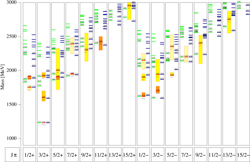
In fig. 2 we compare the results from the present calculation (model $\mathcal{C}$) (right side of each column) with experimental data from the Particle Data Group PDG (central in each column) and with the results from model $\mathcal{A}$ of  LoeMePe2 (left side in each column) . The parameters used are listed in table 2 .

Fig. 2: Comparison of the $\Delta$-Spectrum calculated within the present model $\mathcal{C}$ (right side of each column) with experimental data from the Particle Data Group PDG (central in each column) and with the results from model $\mathcal{A}$ of  LoeMePe2 (left side in each column), note the caption to fig. 1; Lines indicate the resonance position (mass) with the mass uncertainty represented by a shaded box and the rating of PDG indicated by stars. The small numbers give the mass in MeV. $J$ and $\pi$ denote total angular momentum and parity, respectively.

Table 4: Comparison of experimental PDG and calculated masses in MeV of $\Delta$-resonances. The corresponding spectra are shown in fig. 2 .

exp.	rating	model $\mathcal{C}$	exp.	rating	model $\mathcal{C}$
$S_{31}(1620)$	****	1634	$S_{31}(1900)$	***	1932
$S_{31}(2150)$	*	2040/2109
$P_{31}(1750)$	*	1653	$P_{31}(1910)$	****	1888
$P_{33}(1232)$	****	1231	$P_{33}(1600)$	***	1559
$P_{33}(1920)$	***	1894/1925
$D_{33}(1700)$	****	1591	$D_{33}(1940)$	*	1871/1944
$D_{35}(1930)$	***	2012
$F_{35}(1905)$	****	1897	$F_{35}(2000)$	*	1961
$F_{37}(1950)$	****	1936	$F_{37}(2390)$	*	many res.
$G_{37}(2200)$	*	2126/2198	$G_{39}(2400)$	**	2232
$H_{39}(2300)$	**	2319	$H_{3,11}(2420)$	****	2372
$I_{3,13}(2750)$	**	2584
$K_{3,15}(2950)$	**	2724/2909

Table 5: Comparison of experimental PDG and calculated masses in MeV of $N$-resonances. The corresponding spectra are shown in fig. 3 .

exp.	rating	model $\mathcal{C}$	exp.	rating	model $\mathcal{C}$
$S_{11}(1535)$	****	1484	$S_{11}(1650)$	****	1672
$S_{11}(2090)$	*	many res.
$P_{11}(939)$	****	945	$P_{11}(1440)$	****	1440
$P_{11}(1710)$	***	1709	$P_{11}(2100)$	*	many res.
$P_{13}(1720)$	****	1703	$P_{13}(1900)$	**	1825
$D_{13}(1520)$	****	1534	$D_{13}(1700)$	***	1685
$D_{13}(2080)$	**	many res.	$D_{15}(1675)$	****	1667
$D_{15}(2200)$	**	many res.
$F_{15}(1680)$	****	1761	$F_{15}(2000)$	**	1930/1983
$F_{17}(1990)$	**	2001
$G_{17}(2190)$	****	2011	$G_{19}(2250)$	****	2165
$H_{19}(2220)$	****	2192
$I_{1,11}(2600)$	***	2377
$K_{1,13}(2700)$	**	2543

The spectrum of the $\Delta$ (see fig. 2) and $\Omega$ (see right panel of fig. 6) resonances is determined by the confinement potential and the flavour exchange interaction only, since the instanton induced interaction does not act on flavour symmetric states. Concerning the positive parity resonances we see that in the present calculation we can now indeed account for the low position of the $\Delta_{\frac{3}{2}^{+}}(1600)$ resonance. In addition the next excitations in this channel now lie closer to 2000 MeV in better agreement with experimental data, as is also the case for the splitting of the two $\Delta_{\frac{1}{2}^{+}}$ resonances. Note, however, that these states were included in the parameter fit. Additionally there is support for a parity doublet $\Delta_{\frac{3}{2}^{+}}(1920)$ and $\Delta_{\frac{3}{2}^{-}}(1940)$ as argued by Horn .

Likewise, we can now account for the excited negative parity resonances: $\Delta_{\frac{1}{2}^{-}}(1900)$ ,$\Delta_{\frac{3}{2}^{-}}(1940)$ and $\Delta_{\frac{5}{2}^{-}}$ $(1930)$ and even find two states in the $\Delta_{\frac{3}{2}^{-}}$ channel which could correspond to the poorly established $\Delta_{\frac{3}{2}^{-}}(1940)$ state.

In view of the near degeneracy of the $\Delta_{\frac{1}{2}^{-}}$ $(1900)$ , $\Delta_{\frac{3}{2}^{-}}$ $(1940)$ and $\Delta_{\frac{5}{2}^{-}}(1930)$ states it is tempting to classify these in a non-relativistic scheme as a total spin $S=\frac{3}{2}$, total quark angular momentum $L=1$ multiplet, which, because of total isospin $I=\frac{3}{2}$ must then belong to a $(56,1^{-})$ multiplet, which is lowered with respect to the bulk of the other negative parity states that in an oscillator classification would be attributed to the $N=3$ band.

Obviously this is not supported by the calculations: As table 3 shows, although the lowest $J^{\pi}=\frac{5}{2}^{-}$ resonance has a dominant component in this multiplet, the second excited $J^{\pi}=\frac{1}{2}^{-},\frac{3}{2}^{-}$ resonances have dominant components in the $(70,1^{-})$ multiplet; indeed the third excited states in these channels can be attributed to the $(56,1^{-})$ multiplet. Otherwise the description and in particular the $\Delta$-Regge-trajectory are of a similar quality as in the original model $\mathcal{A}$ .

Concerning the $\Omega$ spectrum, see fig. 6 (right panel), apart from the appearance of an excited $\Omega_{\frac{3}{2}^{+}}$ state at 2021 MeV no spectacular changes in the predictions with respect to the original model $\mathcal{A}$ were found. Note that the present model predicts that this state is almost degenerate with the first negative parity states $\Omega_{\frac{1}{2}^{-}}$ at 2008 MeV and $\Omega_{\frac{3}{2}^{-}}$ at 1983 MeV.

In table 4 we have summarised the calculation of $\Delta$-resonances.

4.3 The $N$ spectrum

In fig. 3 we present the results for the nucleon spectrum.

Fig. 3: Comparison of the $N$-Spectrum calculated within the present model $\mathcal{C}$ (right side of each column) with experimental data from the Particle Data Group PDG (central in each column) and with the results from model $\mathcal{A}$ of  LoeMePe2 (left side in each column). See also caption to fig. 2.

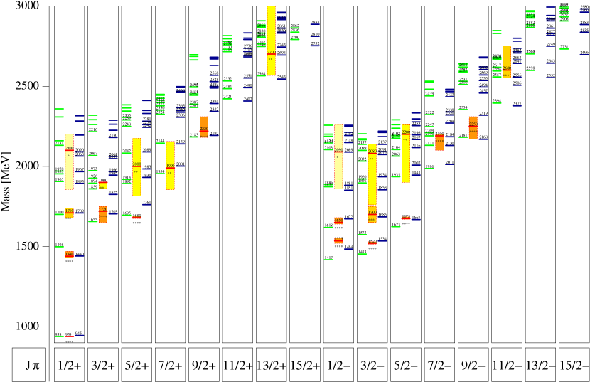
As was the case for the $\Delta$ spectrum, comparing to the results from the former model $\mathcal{A}$ we indeed obtain an improved description of the position of the first excited state with the same quantum numbers as the ground state, the so called Roper resonance, while at the same time improving also on the position of the first excited negative parity resonances $J^{\pi}=\big{(}\tfrac{1}{2}^{-}\big{)}_{1}$,$\big{(}\tfrac{1}{2}^{-}\big{)}_{2}$, $\big{(}\tfrac{3}{2}^{-}\big{)}_{1}$, $\big{(}\tfrac{3}{2}^{-}\big{)}_{2}$ and $\big{(}\tfrac{5}{2}^{-}\big{)}_{1}$ . With the exception of the $J^{\pi}=\frac{5}{2}^{+}$ state, which compared to model $\mathcal{A}$ is shifted upwards by approximately 50 MeV, the description of all known excited states is of a similar quality as that of model $\mathcal{A}$. In particular the position of the lowest $J^{\pi}=\frac{7}{2}^{-}$ resonance is still underestimated by more than 100 MeV.

In the following we compare the predictions obtained in model $\mathcal{C}$ for nucleon resonances with $J\leq\frac{5}{2}$ and masses larger than 1.8 GeV with new results obtained in the Bonn-Gatchina analyses as reported in Anisovich_1 ; Anisovich_2 : In particular in Anisovich_1 a fourth $J^{\pi}=\frac{1}{2}^{+}$ state was found, called $N_{\frac{1}{2}^{+}}(1875)$ which could correspond to our calculated state at 1893 MeV. Furthermore the analysis contains two$J^{\pi}=\frac{3}{2}^{+}$ states, called $N(1900)P_{13}$ and $N_{\frac{3}{2}^{+}}(1975)$, which might be identified with the model $\mathcal{C}$ states calculated at 1825 MeV and 1945 MeV (or 1966 MeV), respectively. Concerning the negative parity states, in Anisovich_2 a new $J^{\pi}=\frac{1}{2}^{-}$ state was found ($N_{\frac{1}{2}^{-}}(1895)$) which could be identified with the calculated state at 1851 MeV (or with that at 1881 MeV). In addition two $J^{\pi}=\frac{3}{2}^{-}$ states were found: $N_{\frac{3}{2}^{-}}(1875)$ could correspond to the calculated states at 1853 MeV (or at 1934 MeV) and $N_{\frac{3}{2}^{-}}(2150)$ with one of the three states with calculated masses 2073 MeV, 2091 MeV and 2137 MeV. The new $N_{\frac{5}{2}^{-}}(2060)$ state reported in Anisovich_2 is closest to the states calculated at 1945 MeV and at 2007 MeV. Finally, for $J^{\pi}=\frac{5}{2}^{+}$ the analysis is ambiguous: Although a solution with a single pole around 2.1 GeV is not excluded, solutions with 2 poles, either an ill-defined pole in the 1800-1950 MeV mass region and one at nearly 2.2 GeV or two close poles at approximately 2.0 GeV were found and could correspond to the model $\mathcal{C}$ states calculated at 1930 MeV and 1983 MeV. Note that these new resonances were not included in the parameter fit (see table 1). An overview of the identification of nucleon resonances is given in table 5.

4.4 Hyperon spectra

Fig. 4: Comparison of the $\Lambda$-Spectrum calculated within the present model $\mathcal{C}$ (right side of each column) with experimental data from the Particle Data Group PDG (central in each column) and with the results from model $\mathcal{A}$ of  LoeMePe2 (left side in each column), see also caption to fig. 2.

Fig. 5: Comparison of the $\Sigma$-Spectrum calculated within the present model $\mathcal{C}$ (right side of each column) with experimental data from the Particle Data Group PDG (central in each column) and with the results from model $\mathcal{A}$ of  LoeMePe2 (left side in each column), see also caption to fig. 2.

\psfrag{Xi}[c][c]{\Huge$\Xi$}\psfrag{Om}[c][c]{\Huge$\Omega$}\includegraphics[width=433.62pt]{Gauss_XisOmegaPS_coupled.eps}

Fig. 6: Comparison of the $\Xi$-Spectrum (first eight columns) and the $\Omega$-Spectrum (rightmost eight columns) calculated within the present model $\mathcal{C}$ (right side of each column) with the experimental data from the Particle Data Group PDG (central in each column) and with the results from model $\mathcal{A}$ of  LoeMePe2 (left side in each column), see also caption to fig. 2.

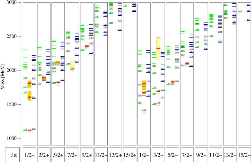
The resulting spectra for hyperon resonances, viz. the $\Lambda$ ,$\Sigma$ and $\Xi$ states are depicted in figs. 4, 5 and 6 , respectively. Again we indeed find an improved description of the “Roper-like” resonances $\Lambda_{\frac{1}{2}^{+}}(1600)$ and $\Sigma_{\frac{3}{2}^{+}}(1660)$. Note, however, that both were used to determine the model parameters. Concerning the negative parity resonances, although we do find an acceptable description of the $\Lambda$ resonances with $J^{\pi}=\frac{3}{2}^{-}\,,\frac{5}{2}^{-}$ and $\frac{7}{2}^{-}\,$, also the new calculation can not account for the low position of the $\Lambda_{\frac{1}{2}^{-}}(1405)$ resonance, which now is 200 MeV below the calculated position. In our opinion this underlines the conclusion, that this state cannot indeed be accounted for in terms of a $q^{3}$ excitation alone and that its position is determined by a strong coupling of a “bare” $q^{3}$ state to meson-baryon decay channels due to the proximity of the $\bar{K}N$-threshold, see also ref. Jido ; Hyodo2008_1 ; Hyodo2008_2 for a description of this state in a chiral unitary approach.

Concerning the $\Xi$ resonances, with respect to model $\mathcal{A}$ of LoeMePe3 mainly the prediction for the excited state $\Xi(\frac{1}{2}^{+})$ at 1765 MeV is 100 MeV lower. To a lesser extend this also holds for the excited $\Xi(\frac{3}{2}^{+})$ which is now predicted at 1889 MeV.

5 Electromagnetic properties

As has been elaborated in Merten in lowest order the transition current matrix element for an initial baryon state with four-momentum $\bar{P}^{\prime}=M=(M,\vec{0})$ in its rest frame and a final baryon state with four-momentum $\bar{P}$ is given by the expression

$$\langle\bar{P}|j^{\mu}(0)|M\rangle=\!-3\!\!\int\!\!\frac{\textrm{d}^{4}p_{\xi}}{(2\pi)^{4}}\!\!\int\!\!\frac{\textrm{d}^{4}p_{\eta}}{(2\pi)^{4}}\!\textstyle{\bar{\Gamma}}^{\Lambda}_{\bar{P}}\!\left(p_{\xi},p_{\eta}\!-\!\frac{2}{3}q\right)$$

$$\hskip 10.00002pt\textstyle S^{1}_{F}\!\left(\frac{1}{3}M+\!p_{\xi}\!+\!\frac{1}{2}p_{\eta}\right)\!\otimes\!S^{2}_{F}\!\left(\frac{1}{3}M-\!p_{\xi}\!+\!\frac{1}{2}p_{\eta}\right)$$

$$\hskip 10.00002pt\textstyle\otimes S^{3}_{F}\!\left(\frac{1}{3}M\!-\!p_{\xi}\!-\!p_{\eta}\!+\!q\right)\widehat{q}\gamma^{\mu}S^{3}_{F}\!\left(\frac{1}{3}M\!-\!p_{\xi}\!-\!p_{\eta}\right)$$

$$\hskip 100.00015pt\textstyle\Gamma^{\Lambda}_{M}\left(\vec{p}_{\xi},\vec{p}_{\eta}\right)\,.$$ (27)

Here $q$ denotes the momentum transfer, $\widehat{q}$ is the charge operator and

$$\Gamma^{\Lambda}_{M}\left(\vec{p}_{\xi},\vec{p}_{\eta}\right):=-\textrm{i}\int\frac{\textrm{d}p^{\prime}_{\xi}}{(2\pi)^{4}}\int\frac{\textrm{d}p^{\prime}_{\eta}}{(2\pi)^{4}}$$ (28)

$$\hskip 10.00002pt\left[V^{(3)}_{\Lambda}\left(\vec{p}_{\xi},\vec{p}_{\eta};\vec{p}^{\prime}_{\xi},\vec{p}^{\prime}_{\eta}\right)+V^{\textrm{eff}}_{\Lambda}\left(\vec{p}_{\xi},\vec{p}_{\eta};\vec{p}^{\prime}_{\xi},\vec{p}^{\prime}_{\eta}\right)\right]$$

$$\hskip 100.00015pt\Phi^{\lambda}_{M}\left(\vec{p}^{\prime}_{\xi},\vec{p}^{\prime}_{\eta}\right)$$

is the vertex function in the rest frame of the baryon with $V_{\Lambda}$ the projection of the instantaneous interaction kernels onto the subspace of purely positive and purely negative energy components only, see in particular Appendix A of Merten for details. The vertex for a general four-momentum on the mass shell can be obtained by an appropriate Lorentz-boost.

Accordingly, the Sachs form factors are given by

$$G^{N}_{E}(Q^{2}) = \frac{\langle N,\bar{P},\frac{1}{2}|j^{E}_{0}(0)|N,M,\frac{1}{2}\rangle}{\sqrt{4M^{2}+Q^{2}}}$$ (29a)

$$G^{N}_{M}(Q^{2}) = \frac{\langle N,\bar{P},\frac{1}{2}|j^{E}_{+}(0)|N,M,-\frac{1}{2}\rangle}{2\sqrt{Q^{2}}}$$ (29b)

where $\left|N,\bar{P},\lambda\right\rangle$ denotes a nucleon state with four-momentum $\bar{P}$ and helicity $\lambda$. Furthermore $Q^{2}=-q^{2}$ and $j^{E}_{\pm}:=j^{E}_{1}\pm\textrm{i}\,j^{E}_{2}$  as well as $|\vec{P}|^{2}=Q^{2}+$ $\frac{(M^{2}-{M^{\prime}}^{2}-Q^{2})^{2}}{4\,M^{2}}$ . Likewise, the axial vector form factor is given by

$$G_{A}(Q^{2}) = \frac{\langle p,\bar{P},\frac{1}{2}|j^{A}_{+}(0)|n,M,-\frac{1}{2}\rangle}{\sqrt{4M^{2}+Q^{2}}}$$ (30)

where again $j^{A}_{\pm}:=j^{A}_{1}\pm$ $\textrm{i}\,j^{A}_{2}$ with $j^{A}_{\mu}$ the axial current operator, whose matrix elements are given by Eq. (5) after the formal substitution $\hat{q}\,\mapsto\,$ $\tau^{+}\gamma^{5}$ . Of course, the normalisations of the form factors is such that the static magnetic moments and the axial coupling are given by

$$\mu_{M}:=G_{M}(Q^{2}=0)\,,\qquad g_{A}:=G_{A}(Q^{2}=0)\,.$$

5.1 The electric form factors of the nucleon

In fig. 7 and 8 we display the electric proton and neutron form factor, respectively, up to a momentum transfer of $Q^{2}=6.0$ $\textrm{GeV}^{2}$. The black solid curve is the result of the present model $\mathcal{C}$, the blue dashed curve is the result obtained with the parameters of model $\mathcal{A}$, as in Merten , albeit with a better numerical precision, see the end of Subsection 2.2 .

Although the electric form factor of the proton, see fig. 7,

\psfrag{x-axis}[c][c]{$Q^{2}\,\,[\textrm{GeV}^{2}]$}\psfrag{y-axis}[c][c]{$G_{E}^{p}(Q^{2})/G_{D}(Q^{2})$}\psfrag{MMD}[r][r]{\scriptsize MMD \cite[cite]{\@@bibref{Authors Phrase1YearPhrase2}{Mergell}{\@@citephrase{(}}{\@@citephrase{)}}}}\psfrag{Christy}[r][r]{\scriptsize Christy \cite[cite]{\@@bibref{Authors Phrase1YearPhrase2}{Christy}{\@@citephrase{(}}{\@@citephrase{)}}}}\psfrag{Qattan}[r][r]{\scriptsize Qattan \cite[cite]{\@@bibref{Authors Phrase1YearPhrase2}{Qattan}{\@@citephrase{(}}{\@@citephrase{)}}}}\psfrag{Merten}[r][r]{\scriptsize model $\mathcal{A}$ \cite[cite]{\@@bibref{Authors Phrase1YearPhrase2}{Merten}{\@@citephrase{(}}{\@@citephrase{)}}}}\psfrag{Gauss}[r][r]{\scriptsize model $\mathcal{C}$}\includegraphics[width=433.62pt]{EFF_Dipole_P.eps}

Fig. 7: The electric form factor of the proton divided by the dipole form $G_{D}(Q^{2})$, Eq. (31). MMD-Data are taken from Mergell et al. Mergell , supplemented by data from Christy et al. Christy and Qattan et al. Qattan  . The solid black line represents the results from the present model $\mathcal{C}$; the dashed blue line those from model $\mathcal{A}$ of Merten , albeit recalculated with higher numerical precision. Red data points are taken from polarisation experiments and black ones are obtained by Rosenbluth separation.

as calculated with model $\mathcal{A}$ in Merten fell too steeply in comparison to experimental data, with the present interaction we find a much improved shape which yields a satisfactory description even up to momentum transfers of 6 GeV² . Indeed, in contrast to model $\mathcal{A}$, which mainly failed with respect to the isovector part of the form factor, in the present model $\mathcal{C}$ this form factor shows an almost perfect dipole shape with the parametrisation

$$G_{D}(Q^{2})=\frac{1}{(1+Q^{2}/M_{V}^{2})^{2}}\,,$$ (31)

taken from Mergell ; Bodek with $M_{V}^{2}=0.71\,\textrm{GeV}^{2}$.

The resulting electric neutron form factor, see fig. 8,

\psfrag{x-axis}[c][c]{$Q^{2}\,\,[\textrm{GeV}^{2}]$}\psfrag{y-axis}[c][c]{$G_{E}^{n}(Q^{2})$}\psfrag{MMD}[r][r]{\scriptsize MMD \cite[cite]{\@@bibref{Authors Phrase1YearPhrase2}{Mergell}{\@@citephrase{(}}{\@@citephrase{)}}}}\psfrag{Rosenbluth}[r][r]{\scriptsize\cite[cite]{\@@bibref{Authors Phrase1YearPhrase2}{Eden,Herberg,Ostrick,Passchier,Schiavilla}{\@@citephrase{(}}{\@@citephrase{)}}}}\psfrag{Polarisation}[r][r]{\scriptsize\cite[cite]{\@@bibref{Authors Phrase1YearPhrase2}{Rohe,Golak,Zhu,Madey,Warren,Glazier,Alarcon}{\@@citephrase{(}}{\@@citephrase{)}}}}\psfrag{Merten}[r][r]{\scriptsize model $\mathcal{A}$ \cite[cite]{\@@bibref{Authors Phrase1YearPhrase2}{Merten}{\@@citephrase{(}}{\@@citephrase{)}}}}\psfrag{PS-coupl}[r][r]{\scriptsize PS Yukawa}\psfrag{PV-coupl}[r][r]{\scriptsize PV Yukawa}\psfrag{Gauss}[r][r]{\scriptsize model $\mathcal{C}$}\includegraphics[width=433.62pt]{EFF_N.eps}

Fig. 8: The electric form factor of the neutron. MMD-Data are taken from the compilation of Mergell et al. Mergell . The solid black line represents the results from the present model $\mathcal{C}$; the green- and brown-dashed lines corresponds to the Yukawa-like models with pseudoscalar and/or pseudovector coupling, see Eqs. (24) and (3.3) respectively; the dashed blue line in the result from model $\mathcal{A}$ of Merten , albeit recalculated with higher numerical precision. Red data points are taken from polarisation experiments and black ones are obtained by Rosenbluth separation.

has a maximum at approximately the experimental value of $Q^{2}\approx 0.4\textrm{ GeV}^{2}$ but underestimates the experimental data from Schiavilla by about the same amount as the earlier calculation overestimated the data. However, the prediction of model $\mathcal{C}$ is very similar to the predictions of the Graz group Plessas and Melde07 for the Goldstone-boson-exchange quark models. The corresponding charge radii are given in table 6 . As for the form factor the resulting squared charge radius of the neutron is calculated too small by a factor of two. Also the r.m.s. proton radius is slightly smaller than the experimental value.

Table 6: Static properties of the nucleon. The values in parentheses are as reported in Merten , the values on top of these are obtained within the same model $\mathcal{A}$ but with higher numerical accuracy. The columns PS and PV are the results obtained with the additional interaction kernels according to Eqs. (24) and (3.3), respectively, see also Section 6 for a brief remark. The static values are extrapolated from a dipole shape-like fit.

	Model $\mathcal{A}$	PS	PV	model $\mathcal{C}$	exp.	ref.
$\mu_{p}[\mu_{N}]\!\!\!\!$	2.76	2.49	2.39	2.54	2.793​​​​	PDG
	[2.74]
$\mu_{n}[\mu_{N}]\!\!\!\!$	-1.71	-1.59	-1.54	-1.59	-1.913​​​​	PDG
	[-1.70]
$\!\!\!\!\sqrt{\langle r^{2}\rangle_{E}^{p}}$[fm]	0.91	0.83	0.68	0.81	0.847​​​​	Mergell
	[0.82]
$\langle r^{2}\rangle_{E}^{n}$[fm]2	-0.20	0.01	0.08	-0.06	-0.123​​​​	Mergell
	[-0.11]				$\pm$0.004
$\!\!\!\!\sqrt{\langle r^{2}\rangle_{M}^{p}}$[fm]	0.90	0.81	0.68	0.78	0.836​​​​	Mergell
	[0.91]
$\!\!\!\!\sqrt{\langle r^{2}\rangle_{M}^{n}}$[fm]	0.84	0.79	0.67	0.75	0.889​​​​	Mergell
	[0.86]
$g_{A}$	1.22	1.17	1.14	1.13	1.267​​​​	PDG ; Bodek
	[1.21]				$\pm$0.0035​​​​
$\!\!\sqrt{\langle r^{2}\rangle_{A}}$[fm]	0.68	0.64	0.48	0.57	0.67​​​​	Bernard
	[0.62]				$\pm$0.01​​​​

Table 7: Octet hyperon magnetic moments $\mu$ for model $\mathcal{A}$ and $\mathcal{C}$ calculated as in Haupt . The values are given in units of $\mu_{N}$.

hyperon	model $\mathcal{A}$	model $\mathcal{C}$	PDG PDG
$\Lambda$	-0.606	-0.577	-0.613 $\pm$0.004
$\Sigma^{+}$	2.510	2.309	2.458 $\pm$0.010
$\Sigma^{0}$	0.743	0.701	-
$\Sigma^{-}$	-1.013	-0.908	-1.160 $\pm$0.025
$\Xi^{0}$	-1.324	-1.240	-1.250 $\pm$0.014
$\Xi^{-}$	-0.533	-0.532	-0.651$\pm$0.0025

Table 8: Decuplet hyperon magnetic moments $\mu$ for model $\mathcal{A}$ and $\mathcal{C}$ calculated as in Haupt . The values are given in units of $\mu_{N}$.

hyperon	model $\mathcal{A}$	model $\mathcal{C}$	PDG PDG
$\Delta^{++}$	4.241	4.238	3.7 to 7.5
$\Delta^{+}$	2.121	2.119	$2.7_{-1.3}^{+1.0}\pm 1.5\pm 3$
$\Delta^{0}$	0.0	0.0
$\Delta^{-}$	-2.121	-2.119
$\Sigma^{\ast+}$	2.567	2.431
$\Sigma^{\ast 0}$	0.275	0.205
$\Sigma^{\ast-}$	-2.017	-2.021
$\Xi^{\ast 0}$	0.607	0.474
$\Xi^{\ast-}$	-1.865	-1.765
$\Omega^{-}$	-1.675	-1.577	$-2.02\pm 0.05$

In fig. 9 and  10 we display the magnetic proton- and neutron form factor up to a momentum transfer of $Q^{2}=6.0\,\textrm{GeV}^{2}$ , respectively. Again, the black solid curve is the result of the present model $\mathcal{C}$, the blue dashed curve is the result obtained with the parameters of model $\mathcal{A}$, as in Merten , albeit with a better numerical precision, see the end of Subsection 2.2 .

\psfrag{x-axis}[c][c]{$Q^{2}\,\,[\textrm{GeV}^{2}]$}\psfrag{y-axis}[c][c]{$G_{M}^{p}(Q^{2})/G_{D}(Q^{2})/\mu_{p}$}\psfrag{MMD}[r][r]{\scriptsize MMD \cite[cite]{\@@bibref{Authors Phrase1YearPhrase2}{Mergell}{\@@citephrase{(}}{\@@citephrase{)}}}}\psfrag{Christy}[r][r]{\scriptsize Christy \cite[cite]{\@@bibref{Authors Phrase1YearPhrase2}{Christy}{\@@citephrase{(}}{\@@citephrase{)}}}}\psfrag{Qattan}[r][r]{\scriptsize Qattan \cite[cite]{\@@bibref{Authors Phrase1YearPhrase2}{Qattan}{\@@citephrase{(}}{\@@citephrase{)}}}}\psfrag{Bartel}[r][r]{\scriptsize Bartel \cite[cite]{\@@bibref{Authors Phrase1YearPhrase2}{Bartel}{\@@citephrase{(}}{\@@citephrase{)}}}}\psfrag{Merten}[r][r]{\scriptsize Merten $\mathcal{A}$ \cite[cite]{\@@bibref{Authors Phrase1YearPhrase2}{Merten}{\@@citephrase{(}}{\@@citephrase{)}}}}\psfrag{Gauss}[r][r]{\scriptsize model $\mathcal{C}$}\includegraphics[width=433.62pt]{MFF_Dipole_P.eps}

Fig. 9: The magnetic form factor of the proton divided by the dipole form $G_{D}(Q^{2})$, Eq. (31) and the magnetic moment of the proton $\mu_{p}=2.793\,\mu_{N}$. MMD-Data are taken from the compilation of Mergell et al. Mergell . Additionally, polarisation experiments are marked by red. The black marked data points are obtained by Rosenbluth separation.

\psfrag{x-axis}[c][c]{$Q^{2}\,\,[\textrm{GeV}^{2}]$}\psfrag{y-axis}[c][c]{$G_{M}^{n}(Q^{2})/G_{D}(Q^{2})/\mu_{n}$}\psfrag{MMD}[r][r]{\scriptsize MMD \cite[cite]{\@@bibref{Authors Phrase1YearPhrase2}{Mergell}{\@@citephrase{(}}{\@@citephrase{)}}}}\psfrag{Anklin}[r][r]{\scriptsize Anklin \cite[cite]{\@@bibref{Authors Phrase1YearPhrase2}{Anklin}{\@@citephrase{(}}{\@@citephrase{)}}}}\psfrag{Kubon}[r][r]{\scriptsize Kubon \cite[cite]{\@@bibref{Authors Phrase1YearPhrase2}{Kubon}{\@@citephrase{(}}{\@@citephrase{)}}}}\psfrag{Xu}[r][r]{\scriptsize Xu \cite[cite]{\@@bibref{Authors Phrase1YearPhrase2}{Xu}{\@@citephrase{(}}{\@@citephrase{)}}}}\psfrag{Madey}[r][r]{\scriptsize Madey \cite[cite]{\@@bibref{Authors Phrase1YearPhrase2}{Madey}{\@@citephrase{(}}{\@@citephrase{)}}}}\psfrag{Alarcon}[r][r]{\scriptsize Alarcon \cite[cite]{\@@bibref{Authors Phrase1YearPhrase2}{Alarcon}{\@@citephrase{(}}{\@@citephrase{)}}}}\psfrag{Merten}[r][r]{\scriptsize model $\mathcal{A}$ \cite[cite]{\@@bibref{Authors Phrase1YearPhrase2}{Merten}{\@@citephrase{(}}{\@@citephrase{)}}}}\psfrag{Gauss}[r][r]{\scriptsize model $\mathcal{C}$}\includegraphics[width=433.62pt]{MFF_Dipole_N.eps}

Fig. 10: The magnetic form factor of the neutron divided by the dipole form $G_{D}(Q^{2})$, Eq. (31) and the magnetic moment of the neutron $\mu_{n}=-1.913\,\mu_{N}$. MMD-Data are taken from the compilation by Mergell et al. Mergell and from more recent results from MAMI Anklin ; Kubon  . Additionally, polarisation experiments are marked by red data points. The black marked ones are obtained by Rosenbluth separation.

Whereas in the original calculation (model $\mathcal{A}$ of Merten ) the absolute value of these form factors dropped slightly too fast as a function of the momentum transfer, in the present calculation we now find a very good description even at the highest momentum transfers. Only at low momentum transfer the values are too small as is reflected by the rather small values for the various magnetic radii, see table 6 and the too small values of the calculated magnetic moments. Note, however that the ratio $\mu_{p}/\mu_{n}\approx 1.597$ for model $\mathcal{C}$ slightly changes (previously $\mu_{p}/\mu_{n}\approx 1.605$ for model $\mathcal{A}$) and is slightly larger than the experimental value $\mu_{p}/\mu_{n}\approx 1.46$ ; all values are remarkably close to the non-relativistic constituent quark model value $\mu_{p}/\mu_{n}=\frac{3}{2}$ . The magnetic moments of flavour octet and decuplet baryons has been calculated accordingly to the method outlined in Haupt . The results are compared to experimental values in Table 7 and 8, respectively. As a consequence of the better description of the momentum transfer dependencies in the individual form factors, we now also find an improved description of the momentum transfer dependence of the form factor ratio $\mu_{p}\,G^{p}_{E}/G^{p}_{M}(Q^{2})$ , which has been the focus on the discussion whether two-photon amplitudes are relevant for the discrepancy Vanderhaeghen found between recent measurements based on polarisation data (red data points of fig. 11) Milbrath ; Jones ; Gayou2001 ; Gayou2002 ; Punjabi ; Hu ; Crawford ; Higinbotham ; Ron ; Zhan versus the traditional Rosenbluth separation (black data points of fig. 11), see e.g. Price ; Bartel ; Berger_1 ; Walker . Whereas in the original model $\mathcal{A}$ this ratio fell much too steep, we now find in model $\mathcal{C}$ a much better description of this quantity, see fig. 11 for a comparison with various data. Up to $Q^{2}\approx 3\,\textrm{GeV}^{2}$ we indeed find the observed linear dependence.

\psfrag{x-axis}[c][c]{$Q^{2}\,\,[\textrm{GeV}^{2}]$}\psfrag{y-axis}[c][c]{$\mu_{p}\,G_{E}^{p}/G_{M}^{p}(Q^{2})$}\psfrag{Rosenbluth}[r][r]{\scriptsize\cite[cite]{\@@bibref{Authors Phrase1YearPhrase2}{Price,Bartel,Berger_1,Walker,Andivahis}{\@@citephrase{(}}{\@@citephrase{)}}}}\psfrag{Polarisation}[r][r]{\scriptsize\cite[cite]{\@@bibref{Authors Phrase1YearPhrase2}{Milbrath,Jones,Gayou2001,Pospischil,Gayou2002,Punjabi,Higinbotham,Hu,Crawford,Ron,Zhan}{\@@citephrase{(}}{\@@citephrase{)}}}}\psfrag{Merten}[r][r]{\scriptsize model $\mathcal{A}$ \cite[cite]{\@@bibref{Authors Phrase1YearPhrase2}{Merten}{\@@citephrase{(}}{\@@citephrase{)}}}}\psfrag{Gauss}[r][r]{\scriptsize model $\mathcal{C}$}\includegraphics[width=433.62pt]{E_MFF_P_ratio.eps}

Fig. 11: The ratio $\mu_{p}\,G_{E}^{p}/G_{M}^{p}$ compared to recent JLAB data (see legend). In the insert the low momentum transfer region is enlarged. The solid black line is the present result, the dashed blue line the result in model $\mathcal{A}$ . Red data points are taken from polarisation experiments and the black ones are obtained from Rosenbluth separation.

Finally, the axial form factor, see fig. 12, was already very well described in model $\mathcal{A}$ of Merten  . Although falling slightly less steeply, the present calculation still gives a very satisfactory description of the data also at higher momentum transfers in the same manner as in Glozman2001 ; Wagenbrunn2001 ; Wagenbrunn2003 . As for the magnetic moments the value of the axial coupling constant is too small, but of course much better than the non-relativistic constituent quark model result $g_{A}=\frac{5}{3}$ . The axial form factor, presented in fig. 12, is divided by the axial dipole form

$$G^{A}_{D}(Q^{2})=\frac{g_{A}}{(1+Q^{2}/M_{A}^{2})^{2}}\,,$$ (32)

with the parameters $M_{A}=1.014\pm 0.014\,\textrm{GeV}$ and $g_{A}=1.267$ taken from Bodek et al. Bodek .

\psfrag{x-axis}[c][c]{$Q^{2}\,\,[\textrm{GeV}^{2}]$}\psfrag{y-axis}[c][c]{$G_{A}^{3}(Q^{2})/G_{D}^{A}(Q^{2})/g_{A}$}\psfrag{Amaldi}[r][r]{\scriptsize Amaldi \cite[cite]{\@@bibref{Authors Phrase1YearPhrase2}{Amaldi}{\@@citephrase{(}}{\@@citephrase{)}}}}\psfrag{Brauel}[r][r]{\scriptsize Brauel \cite[cite]{\@@bibref{Authors Phrase1YearPhrase2}{Brauel}{\@@citephrase{(}}{\@@citephrase{)}}}}\psfrag{Bloom}[r][r]{\scriptsize Bloom \cite[cite]{\@@bibref{Authors Phrase1YearPhrase2}{Bloom}{\@@citephrase{(}}{\@@citephrase{)}}}}\psfrag{Del Guerra}[r][r]{\scriptsize Del Guerra \cite[cite]{\@@bibref{Authors Phrase1YearPhrase2}{DGuerra}{\@@citephrase{(}}{\@@citephrase{)}}}}\psfrag{Joos}[r][r]{\scriptsize Joos \cite[cite]{\@@bibref{Authors Phrase1YearPhrase2}{Joos}{\@@citephrase{(}}{\@@citephrase{)}}}}\psfrag{Baker}[r][r]{\scriptsize Baker \cite[cite]{\@@bibref{Authors Phrase1YearPhrase2}{Baker}{\@@citephrase{(}}{\@@citephrase{)}}}}\psfrag{Miller}[r][r]{\scriptsize Miller \cite[cite]{\@@bibref{Authors Phrase1YearPhrase2}{Miller}{\@@citephrase{(}}{\@@citephrase{)}}}}\psfrag{Kitagaki83}[r][r]{\scriptsize Kitagaki 83 \cite[cite]{\@@bibref{Authors Phrase1YearPhrase2}{Kitagaki83}{\@@citephrase{(}}{\@@citephrase{)}}}}\psfrag{Kitagaki90}[r][r]{\scriptsize Kitagaki 90 \cite[cite]{\@@bibref{Authors Phrase1YearPhrase2}{Kitagaki90}{\@@citephrase{(}}{\@@citephrase{)}}}}\psfrag{Allasia}[r][r]{\scriptsize Allasia \cite[cite]{\@@bibref{Authors Phrase1YearPhrase2}{Allasia}{\@@citephrase{(}}{\@@citephrase{)}}}}\psfrag{Merten}[r][r]{\scriptsize model $\mathcal{A}$ \cite[cite]{\@@bibref{Authors Phrase1YearPhrase2}{Merten}{\@@citephrase{(}}{\@@citephrase{)}}}}\psfrag{Gauss}[r][r]{\scriptsize model $\mathcal{C}$}\includegraphics[width=433.62pt]{AFF_Dipole_3.eps}

Fig. 12: The axial form factor of the nucleon divided by the axial dipole form in Eq. (32) and the axial coupling $g_{A}=-1.267$. The black solid line is the present result, the blue dashed line the result in model $\mathcal{A}$ . Experimental data are taken from the compilation by Bernard et al. Bernard    .

In summary we find, that the new model $\mathcal{C}$, apart from some improvements in the description of the excitation     spectra at the expense of additional parameters of a phenomenologically introduced flavour dependent interaction does allow for a parameter-free description of electromagnetic ground state properties of a similar overall quality as has been obtained before, with some distinctive improvements on the momentum transfer dependence of various form factors. A discussion of the momentum dependence of helicity amplitudes for the electromagnetic excitation of baryon resonances will be given in a subsequent paper Ronniger2  .

6 Summary and conclusion

In the present paper we have tried to demonstrate that by introducing an additional flavour dependent interaction, parametrised with a Gaussian radial dependence with an universal range and two couplings for flavour octet and flavour singlet exchange, it is possible to improve upon some deficiencies found in a former relativistically covariant constituent quark model treatment of baryonic excitation spectra based on (an instantaneous formulation of) the Bethe-Salpeter equation. These improvements include:

• A better description of excited negative parity states slightly below $2$ GeV in the $\Delta$ spectrum;

• A better description of the position of the first scalar, isoscalar excitation of the ground state in all light-flavour sectors;

• An improved description of the momentum dependence of electromagnetic form factors of ground states without the introduction of any additional parameters.

It must be conceded that this additional interaction was introduced purely phenomenologically and required adrastic modification of the parametrisation of confinement and the other flavour dependent interaction of the original model, which had a form as inferred from instanton effects. In spite of this, with only 10 parameters in total we still consider this to be an effective description of the multitude of resonances found for baryons made out of light flavoured quarks.

\psfrag{De}[c][c]{\Huge$\Delta$}\psfrag{Nu}[c][c]{\Huge$N$}\includegraphics[width=346.89731pt]{Summary_Spec.eps}

Fig. 13: Comparison of the $\Delta$-Spectrum (first six columns) and the $N$-Spectrum (rightmost six columns) calculated within the PS and PV coupled models from Eqs. (24) and (3.3) (right and left side of each column) and with the experimental data from the Particle Data Group PDG (central in each column).

Nevertheless, it would have been preferred, if the additional flavour dependent interaction could be related to a genuine physical process, such as light pseudoscalar meson exchange. Indeed, we tried to find parametrisations of confinement and parameters of the instanton induced interaction, that could be combined with interaction kernels as given by the expressions in Eq. (24) or (3.3). However, for pseudoscalar coupling (PS) of a meson nonet to the quarks, we could find a description of the mass spectra with similar features and of a similar quality as in the present model $\mathcal{C}$ only at the expense of introducing flavour SU(3) symmetry breaking and thus introducing more parameters. The latter was also found to be the case for pseudovector coupling (PV) where, moreover, no significant improvement concerning the deficiencies in the spectra mentioned above was found. For the sake of completeness, the nucleon spectrum for PS and PV coupled models from Eqs. (24) and (3.3) is shown in fig. 13. Furthermore, with both Ansatze we were not able to reproduce in particular the electric neutron form factor, see fig. 8 and table 6 for some typical results. Accordingly, we dismissed these possibilities and preferred the phenomenological approach of model $\mathcal{C}$ discussed in the paper.

A parameter-free calculation of longitudinal and transverse helicity amplitudes for electro-excitation is presently performed and the results will be discussed in a subsequent paper Ronniger2  .