Fundamental limitations for quantum and nanoscale thermodynamics

Abstract

The relationship between thermodynamics and statistical physics is valid in the thermodynamic limit - when the number of particles becomes very large. Here, we study thermodynamics in the opposite regime - at both the nano scale, and when quantum effects become important. Applying results from quantum information theory we construct a theory of thermodynamics in these limits. We derive general criteria for thermodynamical state transformations, and as special cases, find two free energies: one that quantifies the deterministically extractable work from a small system in contact with a heat bath, and the other that quantifies the reverse process. We find that there are fundamental limitations on work extraction from nonequilibrium states, owing to finite size effects and quantum coherences. This implies that thermodynamical transitions are generically irreversible at this scale. As one application of these methods, we analyse the efficiency of small heat engines and find that they are irreversible during the adiabatic stages of the cycle.

Corresponding author: Jonathan Oppenheim, e-mail address j.oppenheim$@$ucl.ac.uk

One of the most basic quantities in thermodynamics is the Helmholtz free energy

$$F(\rho)=\langle E(\rho)\rangle-TS(\rho)$$ (1)

with $T$ the temperature of the ambient heat bath that surrounds the system, $S(\rho)$ the entropy of the system, and $\langle E\rangle$ its average energy. It tells us whether a system at constant volume and in contact with a heat bath can make a spontaneous thermodynamical transition from one state to another. A transition can only happen if the free energy of the final state is lower than that of the initial state. The difference in free energy between the initial and final state is also the amount of work which can be extracted from a system in a thermal bath. It also gives the amount of work required to perform the reverse process, since thermodynamics at the macroscopic scale is reversible.

However, the free energy is only valid in the thermodynamical limit – when $\rho$ is composed of many particles and is classical, in the sense that it is in a state which is a probabilistic mixture of different energies. But thermodynamical effects are not only important in the macroscopic regime – they are becoming increasingly important as we probe and manipulate small systems from the micro up to the mesoscopic scale. Already, molecular motors and micro-machines Scovil1959masers ; Geusic1967quatum ; Alicki79 ; howard1997molecular ; geva1992classical ; Hanggi2009brownian ; allahverdyan2000extraction ; feldmann2006lubrication ; linden2010small have been constructed in the labScovil1959masers ; scully2002afterburner ; rousselet1994directional ; Faucheux1995ratchet and thermodynamical effects are increasingly important in quantum devices and in the construction of quantum computers and memoryLandauer ; bennett82 ; baugh2005experimental . Likewise, quantum effects have implications for thermodynamics gemmer2009quantum ; popescu2006entanglement ; del2011thermodynamic .

In this article, we derive necessary and sufficient conditions for thermodynamical state-to-state transitions which are valid even when the thermodynamical limit is not taken, and even when the system is quantum. We call these conditions thermo-majorization. As a special case of this more general result, we derive two free energies valid in this regime. We also quantify the extent to which general state transformations are irrversible, and derive a criteria for when transitions between two states block-diagonal in energy eigenbasis can be made reversible in the micro-regime. We find that there are particular processes which approach the ideal efficiency, provided that certain special conditions are met. Our most basic result concerns the state of a microsystem, which is out of equilibrium, and we ask first, how to define microscopic work, and then we provide the optimal amount of work that can be drawn from the system when in contact with a heat bath, as well as the amount of work required for the reverse process (the work of formation). The obtained amount of work is given by a version of the relative entropy distance of the state from the Gibbs state. Similarly, the work needed to create a system is given by another version of the relative entropy distance to the Gibbs state. These two cases are examples of our full thermo-majorization result which includes characterization of all possible transitions between states block diagonal in the energy eigenbasis in the presence of a heat bath.

I Results

I.1 Conceptual prerequisites

In the macroscopic regime, the standard free energy can be expressed by means of the relative entropy donald1987free , and this can be used to compute the work drawn from non-equilibrium states espositoB-2011 ; thermoiid . However, it is surprising that in the micro-regime, where fluctuations may dominate, the distillable work and work of formation can also be expressed as relative entropies, albeit very different ones. This is because in the microregime, one has a single system with large fluctuations, and it is not at all clear that one can draw work deterministically, as one does in the macroscopic case. One might have imagined that one need to look at the non-deterministic case where one sometimes succeeds in drawing work, and sometimes doesn’t. This approach, while certainly of interest, has the disadvantage that without deterministic work extraction, it can be difficult to separate work from the entropy stored with the work, since if one is not almost certain to draw work, the work will be inherently noisy. To make the distinction between work and noise, one then invariably looks at running a thermodynamic cycle many times, and this doesn’t allow one to fully consider individual systems. In contrast, here, we are able to make strong statements about what will happen to a single system.

Our results were possible due to combining a number of existing concepts. The case of manipulation of entropy, and deterministic transitions when the Hamiltonian is trivial, was undertaken in uniqueinfo , where transition criteria and work extraction were given by majorization conditions. This can be considered a resource theory of “purity” or entropy. In dahlsten2011inadequacy , a probability of failure was allowed for extracting work, allowing work to be quantified by smooth entropies, and this was extended in del2011thermodynamic to the case where one only wants to extract work from one subsystem of a bipartite state, while preserving the other subsystem. In these three cases, since energy was essentially decoupled from entropy, work extraction was a purely information-theoretic task – defined as going from a mixed state to a pure state – enabling a generalisation of Landauer’s principle, saying that a pure state of a two level system without a Hamiltonian is equivalent to $kT\ln 2$ of work. Indeed, one links the concept of work to entropy change, simply through Landauer’s principle.

However, thermodynamics is not merely the study of entropy, but rather the interplay between energy and entropy. Entropy is only half the picture. A key tool we will need to use, is a resource theory which combines the resource theory of purity, with that of “asymmetry” which is the study of manipulations constrained by superselection rulesgour_resource_2008 , of which energy conservation is a special case. Combining these two resource theories allows one to study thermodynamics in all its generality. A paradigm was presented in Beth-thermo and we shall employ its components as a resource theory here, but with two new twists - first, while keeping the system microscopic, we consider its interaction with a large heat-bath. This allows us to combine the above-mentioned approaches together with the quantum information theory of resources, to obtain a novel theory of thermodynamics in the micro-regime. Secondly, we will add a work system into the picture, which will allow us to define work as the process of raising an energy level of this work system. The skeleton of our construction is the theory of resources, and in a parallel paper thermoiid , we show how it reconstructs thermodynamics in the macroregime in the particular case of many identical copies of a micro-system. The present paper concerns itself with the microregime. Remarkably, even when we have a non-trivial Hamiltonian acting on our system, and manipulate systems through a non-trivial interaction Hamiltonian between the system and reservoir, we still find that work extraction and formation are given by elegant information theoretic quantities.

I.2 Thermal Operations

Figure 1: Macroscopic and microscopic work. a) A macroscopic heat engine which performs work by lifting a heavy weight a certain height. b) In the quantum or micro-regime, we can think of work as the ability to excite a two-level system from one energy state to a higher one. Having many of these atoms would allow us to perform macroscopic work – for example, we could use the atoms in a laser. An amount of work $W$ can be used to produce a transition from the state $|0\rangle\langle 0|$, to the state $|1\rangle\langle 1|$, with Hamiltonian $\hat{W}=W|1\rangle\langle 1|$ (we call such a two-level system, the work qubit, or wit). We can use such a system as a basic work storage unit, since our results will not depend on what physical system is used.

We will first consider a quantum system

$$\rho=\sum\sigma(E,E^{\prime},g,g^{\prime})|E,g\rangle\langle E^{\prime},g^{\prime}|$$ (2)

with a fixed Hamiltonian $H$ and eigenstates of energy $E$ given by $|E,g\rangle$, in contact with a heat bath. We are interested in the types of state transitions which are allowed, and in particular, our ability to use the system as a resource to extract work. We will then consider the case where the Hamiltonian of the initial and final state is not the same, so that the system undergoes a non-cyclic evolution.

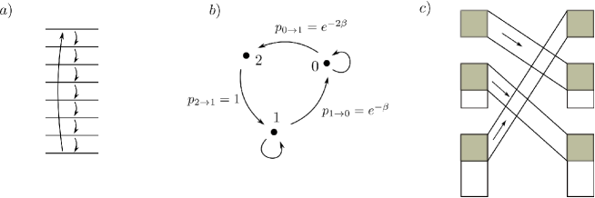
Instead of considering macroscopic work (the pushing out of a piston, or the raising of a weight), we consider microscopic work – for example, the exciting of an atom from its ground state to an excited state (Figure 1). We can thus use a two level system to store work. Because the amount of extractable work can be small, we require precise accounting of all sources of energy. We thus consider a paradigm where extraction of work, and other operations must be done using energy conserving operationsBeth-thermo ; thermoiid , so that any energy which is transferred to or from the resource system and heat bath, is transferred from or to the system which stores work. We do not impose any additional constraints, since we wish to explore fundamental limitations on what can be accomplished on work extraction and formation. We call the class of operations that are allowed Thermal Operations – a fuller discussion of which is contained in Supplementary Note 1, including how it is related to other natural paradigms. This casts thermodynamics as a resource theory Werner1989 ; BDSW1996 ; uniqueinfo ; thermo-ent2002 ; Beth-thermo ; thermoiid , which allows us to exploit some mathematical machinery from information theory. Thermodynamics is then viewed as a theory involving state transformations in the presence of a thermal bath. The extraction or expenditure of work can be included in such a paradigm, because it is equivalent to a state transformation – the state of the work qubit is raised or lowered from one energy eigenstate to another.

Having precisely accounted for all sources of energy, we can apply techniques from single-shot information theory – a branch of information theory specialising in arbitrary resources as opposed to situations where we have many copies of independent and identically distributed bits of information (see e.g. Tomamichel-thesis ). The techniques are thus ideally suited to the case where we want to extract work from a small single system or one whose subsystems are highly correlated. It is also applicable when we wish to extract a deterministic amount of work rather than just extract it statistically, as we can do here by considering systems in contact with a large heat bath which diminish the effect of statistical fluctuations of the system.

I.3 Extractable work

In this more general setting, we show in Supplementary Note 4, that the quantity which replaces the Helmholtz Free Energy for calculating the extractable work in the quantum regime is

$$F_{\min}(\rho)=-kT\ln\sum h(\omega,g,E_{i})e^{-\beta E_{i}}$$ (3)

where $\omega=\sum_{E}P_{E}\rho_{\epsilon}P_{E}$ with $P_{E}=|E\rangle\langle E|$ is the state $\rho$ decohered in the energy eigenbasis (i.e. off-diagonal terms are set to zero), $h(\omega,g,E_{i})$ is $1$ if energy level $|g,E_{i}\rangle$ is populated and $0$ otherwise. $\beta$ is the inverse temperature, and $k$ is Boltzmann’s constant. For microscopic systems, one can generically extract very little work deterministically without allowing a tiny probability $\epsilon$ of failing to draw workdahlsten2011inadequacy . In Supplementary Note 4 we consider this situation and show that a $\beta$-smoothed version of $F_{\min}$, called $F_{\epsilon}^{\min}$, gives the optimal and achievable amount of work extractable from the resource. It’s expression is found in Supplementary Note 4 (Supplementary Equation (S59)) and in the special case that the Hamiltonian is trivial $H=0$, it corresponds to the expression of dahlsten2011inadequacy .

In terms of information theoretic quantities, we can write

$$F_{\min}(\rho)-F_{\min}({\tau})=kTD_{\min}(\rho||\tau)\,\,\,\,,$$ (4)

where $D_{\min}(\omega||\tau):=-\ln\mathop{\mathsf{tr}}\nolimits{\Pi_{\omega}\tau}$ is the min-relative entropypetz ; datta2009min with $\Pi_{\omega}$ the projector onto the support of $\omega$ and $\tau$ is the Gibbs state $\tau=Z^{-1}\sum_{E,g}e^{-\beta E}|E,g\rangle\langle E,g|$ with partition function $Z$. The min-relative entropy and single-shot free energy has been independently introduced as a lower bound for work extraction from classical states using a model of a series of independent interactions with a heat bathaaberg-singleshot .

In the thermodynamical limit $D_{min}(\rho||\tau)$ becomes thermoiid the relative entropy $S(\rho||\tau):=-\mathop{\mathsf{tr}}\nolimits\rho\log\tau+\mathop{\mathsf{tr}}\nolimits\rho\log\rho$ which is equal to $F(\rho)-F(\tau)$donald1987free . Thus, while the maximum amount of work $W$ which can be extracted when a macroscopic system is in contact with a heat bath, is $W(\rho)=F(\rho)-F(\tau)$, more generally it is $W=F_{\epsilon}^{\min}(\rho)-F_{\epsilon}^{\min}(\tau)$ and only in the thermodynamical limit do we recover the traditional result.

Although $F_{\min}$ looks very different to the Helmholtz Free Energy, it can be compared to it easily in the situation where the given state $\rho$ has energy fluctuations $\delta E$ which are small compared with the average energy $\langle E\rangle$ as is the case with macroscopic thermodynamical systems. We then consider a version $\rho_{\epsilon}$ of the state $\rho$, with the tails of weight $\epsilon$ removed (this is more or less what happens when we smooth $F_{\min}$ as discussed in Supplementary Note 4) and find by Taylor expanding $F_{\min}(\rho_{\epsilon})$ around the mean energy and taking the zeroeth order approximation that

$$F_{\min}(\rho_{\epsilon})\approx E-kT\ln\operatorname{rank}(\omega_{\epsilon})$$ (5)

We can now compare this with the Helmholtz Free Energy. In the case where the system is block-diagonal in the energy eigenbasis i.e.

$$\rho=\sum_{E,g,g^{\prime}}\sigma_{E,g,g^{\prime}}|E,g\rangle\langle E,g^{\prime}|\,\,\,\,,$$ (6)

we have that $\rho=\omega$. Then, for extensive systems and the case of many particles $n$, the quantity $\ln\operatorname{rank}(\omega_{\epsilon})=\ln\operatorname{rank}(\rho_{\epsilon})\approx S(\rho)$ with $\epsilon$ going to zero exponentially fast in $n$. (For example, for many non-interacting subsystems such as an ideal case, we may take the system to be composed of many systems in state $\rho^{\otimes n}$. We then obtain the classical resultsthermoiid , and the smoothed min and max entropies approach the von-Neumann entropyRennerphd ; for extensive, isotropic systems, correlations don’t play a role in thermodynamical quantities, and related results hold.) We then have that Equation (5) approaches the Helmholtz Free Energy.

In general however, $\ln\operatorname{rank}(\rho_{\epsilon})$ is larger than the entropy $S(\rho)$, especially in the case where we just have a single system in the micro-regime, meaning that $F_{\epsilon}^{\min}$ is smaller than the free energy. The finite size of the system means that less work can be extracted.

There is a second reason why a limitation exists on the amount of extractable work. A quantum system $\rho$ needn’t be in the form of Equation (6) and in particular can have off-diagonal terms connecting different energy eigenstates. However, it is not $\rho$ which enters into Equation (3), but rather the state $\rho$ decohered in the energy eigenbasis, namely $\omega$. Thus, to zeroeth order, rather than the rank of $\rho_{\epsilon}$ replacing the entropy, it is the rank of $\rho_{\epsilon}$ dephased in the energy eigenbasis that replaces the entropy. This quantity is generally larger than the rank of $\rho_{\epsilon}$ which is why for systems with quantum coherences of energy, there is a further limitation on how much work can be extracted. As an example, consider the pure quantum state

$$|\psi\rangle=\sum_{E}\sqrt{\frac{e^{-\beta E}}{Z}}|E\rangle\,\,\,\,.$$ (7)

It has entropy and rank equal to zero. However, when dephased in the energy eigenbasis to produce $\omega$, it becomes the Gibbs state if the energy levels are non-degenerate, and has free energy $-kT\ln Z$; no work can be extracted from it, despite it having zero entropy. However, as we approach the thermodynamic limit, the coherences matter less and less, and the free energy in the quantum case approaches the free energy for classical statesthermoiid , and again, $F_{\min}$ approaches the Helmholtz Free Energy.

I.4 Work of formation

The fact that at the quantum or nanoscale one can’t extract the work as given by the free energy, implies that there is an inherent irreversibility in thermodynamic transformations. This can also be seen as follows – the maximum amount of work which can be extracted from a system $\rho$ in contact with a heat bath is given by $F_{\epsilon}^{\min}(\rho)-F_{\epsilon}^{\min}(\tau)$. In the process, the system is transformed from state $\rho$ to the Gibbs state $\tau$. But if we wish to use work to perform the reverse process, namely transform Gibbs states into $\rho$ using work, then we show in Supplementary Note 4 that the amount of work which is required is $F_{\epsilon}^{\max}(\rho)-F_{\epsilon}^{\max}(\tau)$ with

$$F_{\epsilon}^{\max}(\rho)=kT\inf_{\rho_{\epsilon}}\log\min\{\lambda:\rho\leq\lambda\tau\}-kT\ln Z$$ (8)

in the case where $\rho$ is diagonal in the energy eigenbasis. Here the infimum is taken over states $||\rho_{\epsilon}-\rho||\leq\epsilon$ with the optimal smoothing given in Supplementary Note 4. In the case where the Hamiltonian is trivial $H=0$, Equation (8) can be interpreted as an upper bound on the amount of work which can be extracted dahlsten2011inadequacy , which coincides with the fact that in such a case, we interpret it as the amount of work which was put into creating the state to begin with. Such an interpretation can also be given to Equation (8) in the case of full thermodynamics with energy.

Again, to compare this quantity to the Helmholtz Free Energy, it’s worth looking at the zeroeth order approximation after expanding in powers of $\delta E/\langle E\rangle$. We find

$$F_{\epsilon}^{\max}(\rho)\approx\inf_{\rho_{\epsilon}}[\langle E\rangle-kT\ln 1/p_{max}]$$ (9)

where $p_{max}$ is the largest probability. To zeroeth order, we see that $F_{\epsilon}^{\min}$ is related to the $\ln\operatorname{rank}$ of the density matrix, the Helmholtz Free Energy to the entropy of the density matrix, and $F_{\epsilon}^{\max}$ to $\ln(1/p_{\max})$. When all probabilities of a density matrix are roughly equal, as is the case for many non-interacting particles $\rho^{\otimes n}$, then these three quantities are equal as well. However, in general, $F_{\epsilon}^{\min}\leq F\leq F_{\epsilon}^{\max}$, so that at the nanoscale we can generally extract less work from a resource than is required to create the resource, leading to a fundamental irreversibility in thermodynamical processes. In terms of information theoretic quantities, $F_{\max}(\rho)-F_{\max}({\tau})=TD_{max}(\rho||\tau)$, where $D_{max}(\rho||\tau):=\log\min\{\lambda:\rho\leq\lambda\tau\}$ is the max-relative entropydatta2009min . As we approach the thermodynamic limit $F_{\epsilon}^{\min}\approx F_{\epsilon}^{\max}$, and reversibility is restoredthermoiid

I.5 More general thermodynamical transformations

More generally, we would like to have criteria which tells us whether one state can be transformed into another under some thermodynamical process. As we have seen, because of finite size or quantum effects, the decreasing of the free energy is not a valid criteria which determines whether a thermodynamic transition can occur. For transitions between a system $\rho$ and a system $\sigma$, both diagonal in the energy eigenbasis, we can derive necessary and sufficient criteria, which we call thermo-majorization. It is based on the majorization condition for state transformations which is a necessary and sufficient condition for state transformations under permutation maps. Its construction is given in Supplementary Note 2, and we state the result in Figure 2. An alternative derivation of our thermo-majorization condition can be obtained by adapting results of Ruch and Mead, studied in the context of decoherence and a particular master equationruch1975diagram ; ruch1976principle ; ruch1978mixing and combining them with our proof that Thermal Operations are Gibbs preserving ones given in Supplementary Note 6 (this latter result in the special case of a heat bath composed of many independent systems was provided in janzing_thermodynamic_2000 ). The derivation we present in Supplementary Note 2 is more direct, and proves the conjecture that the “mixing distance” decreases in thermodynamical systems – a problem which has been open since 1975 ruch1976principle . We are also able to prove the converse.

Figure 2: Thermomajorization. Consider probabilities $p(E,g)$ of the initial system $\rho$ to be in the $g$’th state of energy $E$. Now let us put $p(E,g)\mathrm{e}^{\beta E}$ in decreasing order $p(E_{1},g_{1})\mathrm{e}^{\beta E_{1}}\geq p(E_{2},g_{2})\mathrm{e}^{\beta E_{2}}\geq p(E_{3},g_{3})\mathrm{e}^{\beta E_{3}}...$ – we say that the eigenvalues are $\beta$-ordered. We can do the same for system $\sigma$ i.e. $\mathrm{e}^{\beta E_{1}}q(E_{1},g_{1})\geq\mathrm{e}^{\beta E_{2}}q(E_{2},g_{2})\geq\mathrm{e}^{\beta E_{3}}q(E_{3},g_{3})...$. Then the condition which determines whether we can transform $\rho$ into $\sigma$ is depicted in the above figure. Namely, (a) for any state, we construct a curve with points $k$ given by $\{\sum e^{-\beta E_{i}}/Z,\sum_{i}^{k}p_{i}\}$. Then (b) a thermodynamical transition from $\rho$ to $\sigma$ is possible if and only if, the curve of $\rho$ lies above the curve of $\sigma$. One can make a previously impossible transition possible by adding work in the form of the pure state $\psi_{W}$ which will scale each point by an amount $e^{-\beta W}$ horizontally.

In the case where $\rho$ is not diagonal in the energy eigenbasis, but the final state $\sigma$ is diagonal, then transformations are possible if and only if transformations are possible from $\omega$ to $\sigma$. The reason is simple – dephasing in the energy eigenbasis commutes with Thermal Operationsthermoiid since the latter must conserve energy. Since we can dephase the final state without changing it (as it is already diagonal in the energy basis) we can use the fact that dephasing commutes with our operations to instead dephase the initial state without changing whether the transformation is possible.

In the case where the final state is also non-diagonal in the energy basis, the criteria for which transformations are possible depends on the coupling one has with the system, and especially, the degree of control one has of the system. Thus far, our results have not depended on having fine-grained control of the system and heat bath – the interaction depends on macroscopic variables such as total energy $E$, but the mapping between microstates $g$ does not matterthermoiid . This is not necessarily the case during the formation process of states with off-diagonal terms. Thus, while Equation (3) for the extractable work holds in general, the same is not true of Equation (8) for the formation process. This is because for the formation process of transforming Gibb’s states into a state $\rho$ which is not diagonal in the energy eigenbasis, it is generally not possible to make such a transformation using Thermal Operations without additional resources. In the case of formation of many copies $n$ of $\rho$, the additional resource can be two level pure states in a superposition of energy levelsthermoiid , and the size of the system required scales sublinearly in $n$ and hence vanishes as a fraction of $n$.

I.6 Changing Hamiltonians

So far we have considered transitions between the states of a system with fixed Hamiltonian. This might suggest that our approach does not cover the microscopic analogue of thermodynamical processes between equilibrium states with different initial and final HamiltoniansAlicki79 , such as isothermal expansions of a gas in a container. Yet, fundamentally, a time dependent Hamiltonian is only an effective picture of a fixed Hamiltonian of a larger system, and we shall show below how to describe such transitions in the microscopic regime.

Namely we introduce a qubit on system $C$ which we can act on to switch the Hamiltonian from $H$ to $H^{\prime}$ (we call this the switching qubit). We can for example take the total Hamiltonian to be

$$H_{{\rm tot}}=|0\rangle\langle 0|_{C}\otimes H+|1\rangle\langle 1|_{C}\otimes H^{\prime}+W|1\rangle\langle 1|$$ (10)

and take the initial state of the work qubit, switching qubit and system to be $|00\rangle\langle 00|_{CW}\otimes\rho$ and final state to be $|11\rangle\langle 11|_{CW}\otimes\sigma$, so that we are effectively changing the Hamiltonian acting on $\rho$, and gaining or losing work in the work qubit when we make the transition to $\sigma$. We now consider a transition between $\rho$ and $\tau^{\prime}$, the thermal state with Hamiltonian $H^{\prime}$, and want to know what value (positive or negative) for $W$ allows us to make this transition.

Figure 3: Distillable work, work of formation, and the general case. (a) Graphical representation of two free energies. For Gibbs state they coincide. (b),(c): The scenario of changing Hamiltonian we can mimic by adding to the system $S$ ancilla $C$ switching between initial $H$ and final Hamiltonian $H^{\prime}$, with partition functions $Z,Z^{\prime}$, respectively. We can consider transition $\rho\to\tau^{\prime}$ and $\tau^{\prime}\to\rho$, and obtainable works denote by $W_{\rm dist}$ and $W_{\rm form}$ respectively. The work can be of either signs. Adding/Subtracting work to a state is graphically represented as changing its slope. Formation is depicted by an arrow going from $\rho$ to $\tau^{\prime}$, distillation by arrow going from $\tau^{\prime}$ to $\rho$. The directions of the arrow to the right/left means that the work is positive/negative in a given transition. Positive work, means that we obtain work during the process. We depict two out of possible four cases of work signs: (b) both works are negative (c) work of formation is negative while work of distillation is positive. (d) The interconversion of two arbitrary states is depicted by means of adding/subtracting work; $W$ is the maximal work that can be obtained by the transition $\rho\to\sigma$; $W^{\prime}$ is the minimal work needed to perform the transition $\rho\to\sigma$. Here $\psi_{E}=|1\rangle\langle 1|$ is the excited state of the Hamiltonian $H=E|1\rangle\langle 1|$, for $E=W,W^{\prime},W_{\rm form},W_{\rm dist}$.

The results, obtained by means of thermo-majorization are depicted in Figure 3. One finds

$$W=F_{\epsilon}^{\min}(\omega)-F_{\epsilon}^{\min}(\tau^{\prime})$$ (11)

for extracting work, and for the amount of work required to form $\rho$ (provided it is diagonal in energy eigenbasis) from the thermal state, we obtain

$$W=F_{\epsilon}^{\max}(\rho)-F_{\epsilon}^{\max}(\tau^{\prime})$$ (12)

This result does not depend on the form of the Hamiltonian of Equation (10) – we only require that at late times, there is no interaction between the work qubit and the other systems (since we need to be able to separate out the work qubit to use in some future process). More general state-to-state transformations assisted by work are also depicted.

To derive Equations (11)-(12), we $\beta$-order the $p_{i}$ and $q_{i}$ corresponding to $\rho\otimes|00\rangle\langle 00|$, and $\sigma\otimes|11\rangle\langle 11|$ respectively. Then the thermo-majorization coordinates $k$ of $\rho\otimes|00\rangle\langle 00|$ are given by $\{\sum_{1}^{k}e^{-\beta E_{i}},\sum_{1}^{k}p_{i}\}$, and those of $\sigma\otimes|11\rangle\langle 11|$ are $\{\sum_{1}^{k}e^{-\beta(E^{\prime}_{i}+W)},\sum_{1}^{k}q_{i}\}$. The thermo-majorization condition for a transition is that for all $k$, the points associated with $\rho$ are above that of $\sigma$ and they take a particularly simple form when either $\rho$ or $\sigma$ is the thermal state. These two cases are shown in Figure 3. The case where the final state is thermal for Hamiltonian $H^{\prime}$, $\sigma=\tau^{\prime}$, and the work qubit is excited corresponds to distillation, since no further work can be drawn for fixed $H^{\prime}$ once the state is thermal, and a transition to another state can always be followed by a transition to the thermal state. Therefore drawing work by relaxing the state to a thermal state is completely general, and gives us Equation (11). If $\rho$ has off-diagonal terms, then the distillable work is given by the decohered version $\omega$ in Equation (11), due to the same reasoning as we used earlier – the final state is simply the work qubit, since everything else can be thrown away, and therefore is diagonal in the energy eigenbasis. Since decohering the final state doesn’t change the final state, and decohering with respect to the total Hamiltonian commutes with Thermal Operations, we can do it to the initial state without affecting the amount of work extractable.

The case where we adjust $W$ so that $\rho\otimes|00\rangle\langle 00|_{CW}$ is thermo-majorized by $\sigma\otimes|11\rangle\langle 11|_{CW}$ gives us the formation process, and free energy of Equation (12). The case where both initial and final states $\rho$,$\sigma$ are thermal is also depicted in Figure 3, and leads to the ideal classical result, namely that a transition is possible if and only if

$$W=-kT\ln{Z/Z^{\prime}}$$ (13)

i.e. the work is given by the difference of standard free energies (1).

II Discussion

Equation (13) is a very different result to Equation (3), where we had no ancillary system isolated from the heat bath as in Equation (10). It shows that for thermal equilibrium states there can be reversibility in some thermodynamical processes, provided they are between two thermal equilibrium states and the Hamiltonian changes. In the picture of a fixed Hamiltonian, this required at least one additional system (the switching qubit), which is effectively not in contact with the heat bath, and we do not draw the maximal amount of extractable work from the total working body, given by $F_{\epsilon}^{\min}(\rho_{S}\otimes|0\rangle\langle 0|_{C})$. The final state is thermal only on a subsystem $S$ and therefore the amount of drawn work is not maximal.

This strongly suggests that if we wish to carry out a Carnot cycle to extract work between two heat baths at different temperatures, then to get optimal efficiency during the isothermal process, we will need a working body of at least dimension $2\times 3$. The first two level system acts as the working body which interacts with the heat baths, while the additional three level system is needed if we want to switch between different Hamiltonians in order to achieve the optimal isothermal work extraction given by Equation (13). Even then, we find that while the two isothermal processes can be made ideal, the two adiabatic processes result in additional entropy production, meaning that the Carnot efficiency is not reached over a small number of cycles. This is analysed in Supplementary Note 7.

In general, we only get reversibility if there exists a $W$, such that the thermo-majorization plot of the initial state $\{\sum e^{-\beta E_{i}}/Z,\sum_{i}^{k}p_{i}\}$, can get mapped onto the plot of the final state $\{\sum e^{-\beta(E^{\prime}_{i}+W}/Z^{\prime},\sum_{i}^{k}q_{i}\}$. Thus reversibility requires a very special condition. It is this lack of reversibility which requires two free energies. There is a connection here with other resource theories. Consider the set of states which are preserved under the class of operations – in entanglement theory, these are separable states, and for Thermal Operations, we show in Supplementary Note 6 that it is the Gibbs state. Now, if the theory is reversible, then under certain conditions, the relative entropy distance to the preserved set is the unique measure which governs state transformationsthermo-ent2002 ; BrandaoPlenio2007-separable-maps . For Thermal Operations, the relative entropy distance to the Gibbs state is precisely the free energy differencedonald1987free . Here, in the case of finite sized systems, we see that although we don’t have reversibility, the relative entropy distance to the preserved set again enters the picture, but it is the min and max relative entropy. These quantities are monotonically decreasing under the class of Thermal Operations, and provide two measures for state transitions.

III Methods

The proofs are contained in the Supplementary Information. In Supplementary Note 1, we case thermodynamics as a resource theory, and in Supplementary Note 2, show that the condition for state transformations is given in terms of majorization. In Supplementary Note 3 we consider transitions to and from pure states which we then use in Supplementary Note 4 to derive the extractable work, and work of formation. Supplementary Note 5 discusses the case where we allow the use of ancillas, and Supplementary Note 6 characterises Thermal Operations, and looks at possible transitions in two and three level systems in the case where there are coherences between energy levels. Supplementary Note 7 discusses the details of a small engine undergoing a Carnot cycle.

IV Author Contributions

Both authors contributed equally to this work.

Acknowledgements We thank Robert Alicki, Charles Bennett, Fernando Brandao, Sandu Popescu and Joe Renes for discussions. We thank Lidia del Rio for Figure 1, and comments on our draft. JO is supported by the Royal Society. MH is supported by Polish Ministry of Science and Higher Education grant N N202 231937 and by EC IP QESSENCE. M.H. also acknowledges the support by Foundation for Polish Science TEAM project cofinanced by the EU European Regional Development Fund for preparing the final version of this paper. MH acknowledges the hospitality the of Quantum Computation group at DAMTP, and JO thanks the National Quantum Information Centre of Gdansk and the Dale Farm Residents Association for their hospitality while the manuscript was being completed.

Supplementary Note 1 Thermodynamics as a resource theory

In the micro-regime, when the amount of work which can be extracted might be of the order of $kT$, we need to very precisely define what we mean by work, and what processes are allowed during the extraction of work from a system. For our purposes, obtaining work $\Delta W$ means to obtain an eigenstate of the Hamiltonian with energy $W_{\rm out}$ starting from an eigenstate of energy $W_{\rm in}$, where $W_{\rm in}-W_{\rm out}=\Delta W$. In our approach it will turn out, that the amount of work we can extract from a given system does not depend on the Hamiltonian of the system which stores the work, and the particular levels we choose. We can thus consider a system of the smallest dimension, which carries work $W$. This is a two level system with Hamiltonian $\hat{W}=W|1\rangle\langle 1|$. We shall call this a work qubit (in short, a wit), and let $|\psi_{W}\rangle$ denote the excited state $|1\rangle$ with energy $W$. This is the most economical way of storing work.

Since drawing or adding work can be represented as a state transformation, it is natural to consider thermodynamics as a resource theory. Namely, one considers some class of operations, and then asks how much of some resource can be obtained. Recent examples of such theories include entanglement theory [39,28], thermodynamics with no Hamiltonian [22], thermodynamics of erasure [25] and operations which respect a symmetry [24,40]. Here, we use the class of operations which corresponds to thermodynamics [25,21], and then ask by how much we can excite a system initially in a pure ground state. It can be shown that there are a number of equivalent ways of describing this class of operations [21].

Since we are interested in extracting work in the presence of a heat bath, one starts by allowing a free resource of a heat bath at temperature $T$, and with Hilbert space ${\cal H}_{R}$. The heat bath is in a Gibbs state $\tau$, with arbitrary Hamiltonian and we further allow the addition of any auxiliary system $S^{\prime}$ with Hamiltonian $H_{S^{\prime}}$ in a Gibbs state. Without loss of generality, we can take the initial Hamiltonian to be non-interacting at very early times between the reservoir $R$ and the system of interest $S$, as well as any ancillas. We also want that initially (and finally), the work qubit is not interacting with the rest of the system, since we want to be able to store the work, and use it in some other process. We thus have initially $H_{\rm tot}=H_{R}+H_{S}+H_{S^{\prime}}+\hat{W}$.

We now require that all manipulations conserve energy. This ensures that all sources of work are properly accounted for, and that external systems are not adding or taking away work. The dynamics can be implemented by an interaction Hamiltonian, however, if we wish to maintain a precise accounting of all energy, then the interaction term needs to vanish at the beginning and end of the protocol, otherwise it allows us to pump work into the system at no cost. Essentially we need to ensure conservation of total energy. This also means that if we wish to model a time-dependent Hamiltonian, we should do so by means of a time-independent Hamiltonian with a clock included in the system. It is not difficult to show [21], that all of these paradigms which conserve energy, are equivalent to unitary transformation commuting with the total Hamiltonian. Essentially, since accounting for all sources of energy requires that the initial and final energies are the same, the dynamics must map eigenstates of the Hamiltonian to eigenstates with the same energy. This is equivalent to considering a fixed Hamiltonian, and allowing operations which commute with the Hamiltonian. We also allow discarding subsystems (partial trace). We call this class - Thermal Operations.

Note that this paradigm allows one to include different initial and final Hamiltonians as in the example discussed in the Main Section

$$H_{\rm tot}=|0\rangle\langle 0|_{C}\otimes H+|1\rangle\langle 1|_{C}\otimes H^{\prime}+W|1\rangle\langle 1|$$ (S1)

Via a similar mechanism, one can include interacting terms which vanish at early and late times. Similarly, the application of a unitary during some time period can be made via application of a fixed Hamiltonian [21] and using an ancilla which acts as a clock. Generally, we are interested in transitions between $(\rho_{S},H_{S})$ and $(\sigma_{S^{\prime}}$ and $H_{S^{\prime}})$ (extracting work will be a special case of such a transition). Since in the described approach, the Hamiltonian is fixed, such a transition means actually $(\rho_{S}\otimes\tau_{S^{\prime}},H_{S}+H_{S^{\prime}})\to(\tau_{S}\otimes\sigma_{S^{\prime}},H_{S}+H_{S^{\prime}})$ where we have the same initial and final Hamiltonian.

We will here, generally write an arbitrary transition as just $(\rho_{S},H_{S})\to(\sigma_{S},H_{S})$ since the system $S$ can include a number of components including a clock, a working body, and various other ancillas and coupling systems. Likewise, $H_{S}$ could include various coupling terms. We then derive necessary and sufficient criteria for a transition to be possible. However, one might want to derive conditions for a transitions on some system, while optimising over all configurations of the ancillas and working body. We do that in more detail in [41], where we show to what extent and under what conditions our formulas for work extraction and work of formation are robust under such an optimisation. Here we recall the main conclusions. The most general scenario is the following: apart from the systems considered so far (i.e. heat bath, working body, and work collector) we have also clock and allow any ancillas. This includes the system that allows us to switch on and off any interaction Hamiltonian between the various systems. The total systems evolve altogether under some time-independent Hamiltonian. Now, to comply with Planck’s formulation of second law, we should at the end of a cycle, not change the environment. This means that the state of the clock and other ancillas should be returned intact. This latter condition is however too stringent, since in such case the clock would not be able to perform its task of switching on and off the interaction. Therefore, we have to allow for returning ancillas close to their original state in some distance measure. This then, is the scenario of catalytic transformations, something which has been studied in the case of the resource theory of entanglement [42]. We discuss this in [41] and give the results in Supplementary Note 5, showing that it does not affect our formulas for the min and max free energy for some natural choice of distance measure.

In what follows, we do not consider additional restrictions on the class of operations – we allow any Hamiltonian, and any couplings. Thus our work provides fundamental limitations to thermal transitions in the lab. One might want to consider a more limited class of operations, or add in various practical considerations depending on the physical situation, such as restricting the degree of control one has over the resources, or adding in additional couplings between our heat engines and the thermal baths. However, we have found [21] (see also unpublished results, M. Horodecki and J. Oppenheim) that the operations needed to distill work can be crude, without fine-grained control. Nonetheless, for some Hamiltonians, one might demand even less control, in which case, we provide fundamental limitations, rather than matching limitations and achievability bounds. The same is true for the case where one imposes a further restriction on the class of operations of only coupling the system to a very small reservoir, or small part of the reservoir. In such a case, our fundamental limitations are still of course respected, but the bounds might not be achievable, in part because sampling a region of a reservoir which is small compared with the length of interactions results in the system seeing an effective temperature or non-thermal state, rather than the true temperature [43-45].

Assumptions on heat bath, and its relation to the system

We can assume that Hamiltonians of all systems of concern (i.e. heat bath Hamiltonian, auxiliary systems, the resource system itself) have minimal energy zero. Let $E_{R}$ be the energies of reservoir, and $E_{S}$ be the energies of the system. Let $E_{R}^{\max}$, and $E_{S}^{\max}$ be the largest energy of the heat bath and system, respectively (of course a typical heat bath will have $E_{R}^{\max}=\infty$).

Our heat bath will be large, while our resource states will be small. This means that the system Hilbert space will be fixed, while the energy of the heat bath (and other relevant quantities such as size of degeneracies) will tend to infinity.

We now make some assumptions concerning the state and Hamiltonian of the heat bath and then justify them. The heat bath is in a Gibbs state with inverse temperature $\beta$. Moreover there exists set of energies ${{\cal E}_{R}}$ such that the state of the heat bath occupies energies from ${{\cal E}_{R}}$ with high probability, i.e. for the projector $P_{{\cal E}_{R}}$ onto the states with energies ${{\cal E}_{R}}$ we have

$$\begin{aligned} \mathop{\mathsf{tr}}\nolimits P_{{\cal E}_{R}}\rho_{R}\geq 1-\delta\end{aligned}$$ (S2)

and it has the following properties:

1. The energies $E$ in ${{\cal E}_{R}}$ are peaked around some mean value, i.e. they satisfy $E\in\{\langle E\rangle-O(\sqrt{\langle E\rangle}),\ldots\langle E\rangle+O(\sqrt{\langle E\rangle})\}$

2. For $E\in{{\cal E}_{R}}$ the degeneracies $g_{R}(E)$ scale exponentially with $E$, i.e.

   $$\begin{aligned} g_{R}(E)\geq e^{cE}\end{aligned}$$ (S3)

   where $c$ is a constant.

3. For any three energies $E_{R},E_{S}$ and $E_{s}^{\prime}$ such that $E_{R}\in{{\cal E}_{R}}$ and $E_{S}$, $E_{S}^{\prime}$ are arbitrary energies of the system, there exist $E^{\prime}_{R}\in{{\cal E}_{R}}$ such that $E_{R}+E_{S}=E_{R}^{\prime}+E_{S}^{\prime}$.

4. For $E\in{{\cal E}_{R}}$ the degeneracies $g_{R}(E)$ satisfy $g_{R}(E-E_{S})\approx g_{R}(E)e^{-\beta E_{S}}$, or more precisely:

   $$\begin{aligned} \left|\frac{g_{R}(E)e^{-\beta E_{S}^{\prime}}}{g_{R}(E-E_{S})}-1\right|\leq\delta\end{aligned}$$ (S4)

   for all energies $E_{S}$ of the system $S$.

Discussion of assumptions:

• This is a standard property of a heat bath.

• Follows from the condition (i) of small fluctuations combined with extensivity of energy.

• Follows from continuity of the spectrum of the heat bath, which is usually the case.

• Follows from

  $$g(E+\Delta E) =e^{S(E+\Delta E)}$$

  $$\approx e^{S(E)+\Delta E\frac{\partial S(E)}{\partial E}}$$

  $$=g(E)e^{\beta\Delta E}$$ (S5)

  with $S(E):=\ln g(E)$. and $\beta:=\frac{\partial S(E)}{\partial E}$.

It is also easy to see that a product $\tau^{\otimes n}$ of many copies of independent Gibbs states satisfies the above assumptions.

Notation and preliminary facts

We shall now need a bit of notation. Let us define $\eta^{X}_{E}$ as a state of a system X proportional to the projection on to a subspace of energy $E$ (according to the Hamiltonian $H_{X}$ on this system). In particular, $\eta_{E-E_{S}}$ is given by

$$\begin{aligned} \eta_{E-E_{S}}=g(E-E_{S})^{-1}\sum_{g}|E-E_{S},g\rangle_{R}\langle E-E_{S},g|\end{aligned}$$ (S6)

where $g=1,..,g(E-E_{S})$, i.e. $\eta_{E-E_{S}}$ is the maximally mixed state of the reservoir with support on the subspace of energy $E_{R}=E-E_{S}$. We shall also use notation $\eta_{K}=\mathbb{I}/K$ where the identity acts on a $K$ dimensional space.

Let us note that the total space ${\cal H}_{R}\otimes{\cal H}_{S}$ can be decomposed as follows

$$\begin{aligned} {\cal H}_{R}\otimes{\cal H}_{S}=\bigoplus_{E}\left(\bigoplus_{E_{S}}{\cal H}^{R}_{E-E_{S}}\otimes{\cal H}^{S}_{E_{S}}\right)\end{aligned}$$ (S7)

(here for $E\leq E_{S}$ and $E\geq E_{R}^{\max}+E_{S}^{\max}$ the summation over $E_{S}$ is suitably constrained, however we are interested only in energies $E_{R}$ from ${{\cal E}_{R}}$, hence these cases will not occur).

Consider an arbitrary state $\rho_{RS}$ which has support within $E_{S}^{\max}\leq E\leq E_{R}^{\max}$. We can rewrite it as follows

$$\begin{aligned} \rho_{RS}=\sum_{E}\sum_{\Delta}P_{E}\rho_{RS}P_{E+\Delta}\\ \end{aligned}$$ (S8)

Here $\Delta=-E_{S}^{\max},\ldots,E_{S}^{\max}$. The blocks $P_{E}\rho_{RS}P_{E+\Delta}$ we can further divide into sub-blocks

$$\begin{aligned} P_{E}\rho_{RS}P_{E+\Delta}=\sum_{E_{S}\in I_{\Delta}}\mathbb{I}_{R}\otimes P_{E_{S}}P_{E}\rho_{RS}P_{E+\Delta}\mathbb{I}_{R}\otimes P_{E_{S}+\Delta}\end{aligned}$$ (S9)

where $I_{\Delta}=\{0,\ldots,E_{S}^{\max}-\Delta\}$ for $\Delta\geq 0$ and $I_{\Delta}=\{-\Delta,\ldots,E_{S}^{\max}\}$ for $\Delta\leq 0$. The sub-blocks map the Hilbert space ${\cal H}^{R}_{E-E_{S}}\otimes{\cal H}^{S}_{E_{S}+\Delta}$ onto ${\cal H}^{R}_{E-E_{S}}\otimes{\cal H}^{S}_{E_{S}}$

We can then extract the state $\rho_{S}$

$$\begin{aligned} \rho_{S}=\sum_{E_{S},E_{S}^{\prime}}P_{E_{S}}\rho_{S}P_{E_{S}^{\prime}}\end{aligned}$$ (S10)

as follows:

$$\begin{aligned} P_{E_{S}}\rho_{S}P_{E_{S}^{\prime}}=\sum_{E}\mathop{\mathsf{tr}}\nolimits_{{\cal H}^{R}_{E-E_{S}}}(P^{R}_{E-E_{S}}\otimes P_{E_{S}}P_{E}\rho_{RS}P_{E+E_{S}^{\prime}-E_{S}}P^{R}_{E-E_{S}}\otimes P_{E_{S}^{\prime}})\end{aligned}$$ (S11)

We then have the following technical result that will be a basis for most of our derivations:

Theorem 1.

We consider the set of energies

$$\begin{aligned} {\cal E}=\{E:E-E_{S}\in{{\cal E}_{R}}\}\end{aligned}$$ (S12)

where ${{\cal E}_{R}}$ satisfies assumptions (i), (ii) and (iii) listed above. Then

$$\begin{aligned} \forall{E\in{\cal E}}\quad||\frac{1}{p_{E}}P_{E}\rho_{R}\otimes\rho_{S}P_{E+\Delta}-\oplus_{E_{S}}\eta_{E-E_{S}}\otimes P_{E_{S}}\rho_{S}P_{E_{S}+\Delta}||\leq 2\delta\end{aligned}$$ (S13)

and

$$\begin{aligned} \sum_{E\in{\cal E}}p_{E}\geq 1-2\delta\end{aligned}$$ (S14)

where $p_{E}=\mathop{\mathsf{tr}}\nolimits(P_{E}\rho_{R}\otimes\rho_{S})$.

Proof. Here we sketch the proof for $\Delta=0$. For $\Delta\not=0$ the proof is similar. Let us fix an energy block $E$. Let $E_{R}=E-E_{S}$. The state $\tau_{R}\otimes\rho_{S}$ restricted to the energy $E$ block is given by

$$\begin{aligned} P_{E}\tau_{R}\otimes\rho_{S}P_{E}=\frac{1}{Z_{R}}\sum_{E_{S}}e^{-}{\beta E-E_{S}}g_{R}(E-E_{S})\mathbb{I}_{R}^{E-E_{S}}\otimes P_{E_{S}}\rho_{S}P_{E_{S}}\end{aligned}$$ (S15)

where $Z$ is the partition function for system $R$, and $\mathbb{I}_{R}^{E-E_{S}}$ is the identity on the subspace ${\cal H}_{R}^{E-E_{S}}$, see (S7). Using (iv) we have $g_{R}(E-E_{S})=g_{R}(E)e^{-\beta E_{S}}$ we get

$$\begin{aligned} P_{E}\tau_{R}\otimes\rho_{S}P_{E}\approx\frac{1}{Z_{R}}e^{-\beta E}g_{R}(E)\sum_{E_{S}}\frac{\mathbb{I}_{R}^{E-E_{S}}}{g_{R}(E)e^{-}{\beta E_{S}}}\otimes P_{E_{S}}\rho_{S}P_{E_{S}}\end{aligned}$$ (S16)

We then use $\frac{\mathbb{I}_{R}^{E-E_{S}}}{g_{R}(E)e^{-}{\beta E_{S}}}=\eta_{E-E_{S}}$ and if we drop the prefactor, the state is normalised, hence we obtain the claim.

Supplementary Note 2 Transformations of classical states: condition in terms of majorization

Here we will provide a necessary and sufficient condition for transforming the diagonal part of a density matrix of one state into the diagonal part of another state acting on the same system. The condition will be in terms of the so called majorization condition, and it will be necessary and sufficient for state transformations of classical states (i.e. diagonal in the energy eigenbasis). The result is contained in Theorem 2

Theorem 2.

Consider two states $\rho_{S}$ and $\sigma_{S}$ block-diagonal in the energy eigenbasis, on a system with Hamiltonian $H_{S}$. The transition $(\rho_{S},H_{S})\otimes(\sigma_{S},H_{S})$ by means of Thermal Operations is possible if and only if the state

$$\begin{aligned} \oplus_{E_{S}}\eta_{E-E_{S}}\otimes P_{E_{S}}\rho_{S}P_{E_{S}}\end{aligned}$$ (S17)

majorizes

$$\begin{aligned} \oplus_{E_{S}}\eta_{E-E_{S}}\otimes\sigma_{E_{S}}\end{aligned}$$ (S18)

for $E$ large enough. Moreover, if the above majorization relation holds for two states $\rho_{S}$ and $\sigma_{S}$ not necessarily diagonal in the energy eigenbasis, then there exists $\sigma_{S}^{\prime}$ such that for all $E_{S}$ $P_{E_{S}}\sigma_{S}P_{E_{S}}=P_{E_{S}}\sigma_{S}^{\prime}P_{E_{S}}$, and the transition $(\rho_{S},H_{S})\to(\sigma_{S}^{\prime},H_{S})$ is possible.

The majorization condition reads as follows: we have two sets of eigenvalues put in decreasing order $\{\lambda_{i}\}$ and $\{\lambda^{\prime}_{i}\}$, and we say that $\{\lambda_{i}\}$ majorizes $\{\lambda^{\prime}_{i}\}$ when

$$\begin{aligned} \sum_{i=1}^{l}\lambda_{i}\geq\sum_{i=1}^{l}\lambda_{i}^{\prime}\end{aligned}$$ (S19)

for all $l$. We say that $\rho$ majorizes $\sigma$ if the eigenvalues of $\rho$ majorize the eigenvalues of $\sigma$.

Proof of Theorem 2. The operations that we can perform on the total system, are arbitrary unitary within subspaces of fixed energy. From the expression (S13) it follows that a subspace of fixed energy $E$ contains only the part of $\rho_{S}$ that is block-diagonal in energy of the system $S$:

$$\begin{aligned} P_{E}\rho_{R}\otimes\rho_{S}P_{E}\approx\oplus_{E_{S}}\eta_{E-E_{S}}\otimes P_{E_{S}}\rho_{S}P_{E_{S}}\end{aligned}$$ (S20)

Let us denote by $\rho_{S}^{E}$ the state resulting from applying unitary $U_{E}$ to the above state, and tracing out the heat bath. We shall argue, that if $E$ is large enough, then one can choose such unitary $U_{E}$ that the resulting $\rho_{S}^{E}$ will be the same, as if we had applied to state (S20) an arbitrary mixture of unitaries. Before we prove it, let us continue with the proof of the theorem. Namely, on one hand, by applying $U_{E}$ to each subspace, and tracing out the heat bath, we obtain an output state of the form $\sum_{E}p_{E}\rho_{S}^{E}$ i.e. it is a result of a mixture of operations applied to each single subspace. However, as we’ve stated, already in a single subspace, we can perform an operation which will have the same effect as an arbitrary mixture of unitaries applied to the total state followed by tracing out the heat bath.

Thus we obtain that the most general transition of the block-diagonal part of $\rho_{S}$ can be described by a mixture of unitaries applied to the state (S20) and a partial trace over the heat bath. Hence, according to [46], which says that we can transform a state into another state by a mixture of unitaries if and only if the first one majorizes the second one, we can obtain an arbitrary output state that is majorized by the state (S20). Now, we note that we can further transform such an output state into a state of the form (S18) without changing the state of subsystem $S$. This is done by a ”twirling” operation (which is itself some mixture of unitaries): For each fixed $E_{S}$ we apply a random unitary to the heat bath part, and identity to the part $S^{E}$. After twirling, any state becomes of the above form. This proves the first part of theorem.

The second part follows from the fact that the blocks of fixed total energy contain only the block-diagonal part of $\rho_{S}$, and therefore, if we start with a state which is not diagonal, then we do not know what happens to off-diagonal terms but, by the above discussion, we do know how the diagonal part is transformed. Thus, if state (S20) majorizes a state of the form (S18), then the diagonals of $\rho_{S}$ will be transformed into that of $\sigma_{S}$.

Finally, we need to prove the claim that we can effectively implement any mixture of unitaries, within a single subspace of fixed energy. To see this, note that we can tensor out a maximally mixed state of size independent of both $E_{S}$ and $E$, and apply unitaries conditioned on the maximally mixed state. We do that by writing

$$\begin{aligned} \eta_{E-E_{S}}=\frac{\mathbb{I}_{K}}{K}\otimes\frac{\mathbb{I}_{K^{\prime}_{E_{S}}}}{K^{\prime}_{E_{S}}}\end{aligned}$$ (S21)

where $K^{\prime}_{E_{S}}=g(E-E_{S})/K$. Due to our assumptions about the heat bath, the degeneracy of each energy state is exponentially large in energy, so we can take such $K$ that both $K$ and $K^{\prime}$ are exponentially large in energy. Thus a given fixed energy block $E$ can be represented as a tensor product of two systems $R_{1}^{E}$ and $R_{2}^{E}S^{E}$ in a state

$$\begin{aligned} \frac{1}{p_{E}}P_{E}\rho_{R}\otimes\rho_{S}P_{E}\approx\frac{\mathbb{I}_{K}}{K}\oplus_{E_{S}}\frac{\mathbb{I}_{K^{\prime}_{E_{S}}}}{K^{\prime}_{E_{S}}}\otimes P_{E_{S}}\rho_{S}P_{E_{S}}\end{aligned}$$ (S22)

We then know [22] that any mixture of unitary transformations can be performed on the system $R_{2}^{E}S^{E}$, provided $K$ is large with respect to $K^{\prime}_{E}$, and we shall choose $K$, and the size of the total system, in such a way, that this is so, and at the same time $K^{\prime}_{E}$ can be large too, which we will need further.

Now, the state with $\frac{\mathbb{I}}{K}$ tensored out does not actually differ much from the state $\eqref{eq:eta_form}$, as we anyway will take the system $R_{2}^{E}$ to be large. Thus the output state coming from a mixture of unitaries performed on the state with and without $\frac{\mathbb{I}}{K}$ being tensored out have the same effect on the final form of the state of the system $S$. This ends the proof of theorem.

Note that in the proof we have used the assumptions (i-iii) about the heat bath but not (iv). The latter will be used when we will need to get rid of the heat bath in the majorization expressions in the next section.

Finally, it is intuitively obvious, that if we add to a heat bath a small system in a Gibbs state, this is again a larger heat bath, i.e. it still satisfies our assumptions. Indeed, consider a heat bath $R$ which satisfies assumptions (i-iv), and another system $S^{\prime}$, and consider the total Hamiltonian being a sum of Hamiltonians $H_{R}$ +$H_{S^{\prime}}$. The tensor product of two Gibbs states is a Gibbs state of the total system. Since the original heat bath is large, and our system is small, then the conditions (i), (ii) and (iii) are obviously satisfied. Then, writing

$$\begin{aligned} g^{RS^{\prime}}(E)=\sum_{E_{S^{\prime}}}g^{R}(E-E_{S^{\prime}})g^{S^{\prime}}(E_{S^{\prime}})\end{aligned}$$ (S23)

and using the property (iv) of $g^{R}$ one gets

$$\begin{aligned} g^{RS^{\prime}}(E)\approx g^{R}(E)Z_{S^{\prime}}\end{aligned}$$ (S24)

where $Z_{S^{\prime}}$ is the partition function for $S^{\prime}$. This implies, in particular, that $g^{RS^{\prime}}$ also satisfies the condition (iv).

This proves the following intuitively obvious lemma:

Lemma 3.

Transition between $\rho_{S}\otimes\tau_{S^{\prime}}\to\sigma_{S}\otimes\tau_{S^{\prime}}$ is possible if and only if transition $\rho_{S}\to\sigma_{S}$ is possible.

Thus adding a system in a Gibbs state makes sense only, if we consider transition between systems with different Hamiltonian. Then we bring in a system in a Gibbs state, only in order to have that Hamiltonian in future processes e.g. we might then transform the Gibbs state into another state which needed to have that Hamiltonian.

The conditions given thus far for state transformations are all that is needed to draw the full amount of work from a state, or to form a state from a heat bath. This is done in Supplementary Note 3 For the remainder of this section, we continue with more general state transformations.

Thermo-majorization

We shall now provide an efficient method of finding, whether a transition $(\rho,H)\to(\sigma,H)$ is possible, for states which commute with Hamiltonian $H$. The condition of transformations of the diagonal part of a density matrix given by Theorem 2 in terms of majorization involves not only the state, but also the heat bath, hence it is not always directly useful. We shall now express the condition given by majorization in terms of the states of system $S$ themselves which will result in an efficient algorithm to decide whether a transition between two diagonal states is possible or not. Essentially, we need to write the eigenvalues of the state and heat bath, in terms of eigenvalues of only the state. We shall assume that our input state and output states are diagonal in their energy bases, however, even if they are not, the condition we derive determines possible transformations of the diagonal part of the density matrix, thus the condition becomes necessary, but ceases to be sufficient.

Let $p_{E_{S},g}$ be eigenvalues of $\rho$ and $q_{E_{S},g}$ be eigenvalues of $\sigma$. Then, due to proposition 2 and the condition (iv), the state $P_{E}\rho_{R}\otimes\rho_{S}P_{E}$ after normalisation is close to the state having the following eigenvalues:

$$\begin{aligned} e^{\beta E_{S}}\frac{p(E_{S},g)}{g_{R}(E)}\end{aligned}$$ (S25)

with multiplicity $g_{R}(E)e^{-\beta E_{S}}$, where $E_{S}$ runs over all energies of the system, and $g$ runs over degeneracies. Similarly, $P_{E}\rho_{R}\otimes\sigma_{S}P_{E}$ has eigenvalues $e^{\beta E_{S}}\frac{q(E_{S},g)}{g_{R}(E)}$ with the same multiplicity.

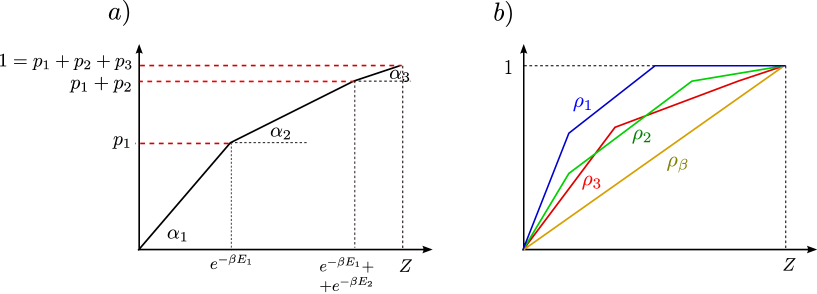
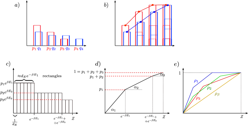
The eigenvalues are very small, and they are collected in groups, where they are the same, hence the majorization amounts to comparing integrals. If one puts eigenvalues into decreasing order, one obtains a stair-case like function, and majorization in this limit will be to compare the integrated functions (which are then piece-wise linear functions).

To see how it works, we need to put the eigenvalues in nonincreasing order. The ordering is determined by the ordering of the quantities $e^{\beta E_{S}}p_{E_{S},g}$. This determines the order of $p(E_{S},g)$ (which in general will not be in decreasing order anymore). We shall denote such ordered probabilities as $p_{i}$, and the associated energy of the eigenstate as $E_{i}$. E.g. $p_{1}$ is equal to the $p(E_{S},g)$ such that $e^{\beta E_{S}}p(E_{S},g)$ is the largest. Note that for fixed $E_{S}$ the order is the same as the order of $p({E_{S},g})$, while for different $E_{S}$ it is altered by the Gibbs factor. We do the same for $\sigma$, which results in $q_{i}$.

The eigenvalues are thus ordered by taking into account Gibbs weights:

$$\begin{aligned} \underbrace{\frac{p_{1}e^{\beta E_{1}}}{{d_{E}}}}_{{\text{multiplicity}\atop\approx d_{E}e^{-\beta E_{1}}}}\geq\underbrace{\frac{p_{2}e^{\beta E_{2}}}{{d_{E}}}}_{{\text{multiplicity}\atop\approx d_{E}e^{-\beta E_{2}}}}\geq\ldots\end{aligned}$$ (S26)

where $d_{E}$ is a shorthand for $g_{R}(E)$. We shall now ascribe to vector $\{p_{i}\}$ a function mapping interval $[0,Z]$ into itself. On the $y$ axis, we put subsequent sums $\sum_{i=1}^{l}p_{i}$, $l=1,\ldots,d$ where $d$ is the number of all probabilities, and on the $x$ axis, we put sums $\sum_{i=1}^{l}e^{-\beta E_{i}}$, with the final point being at $x=Z$. This gives $d+1$ pairs: $(0,0),(p_{1},e^{-\beta E_{1}}),(p_{1}+p_{2},e^{-\beta E_{1}}+e^{-\beta E_{2}}),\ldots,(Z,1)$. We join the points, and it will gives us a graph of a function, $f_{p}(x)$. It is easy to see, that in the limit of large $g_{R}(E)$, the eigenvalues of $\rho$ majorize eigenvalues of $\sigma$ if and only if $f_{p}(x)\geq f_{q}(x)$ for all $x\in[0,Z]$. The described scheme is presented in Supplementary Figure S1.

Supplementary Figure S1: Thermo-majorization. I. Standard majorization: (a) the histograms of probability distributions $\{p_{i}\}$ and $\{q_{i}\}$. (b) The distribution $\{p_{i}\}$ majorizes distribution $\{q_{i}\}$ if for all $l$ $\sum_{i=1}^{l}p_{i}\geq\sum_{i=1}^{l}q_{l}$. Graphically,this means that the entire plot corresponding to $\{p_{i}\}$ is above the plot corresponding to $\{q_{i}\}$. II. Thermo-majorization. (c) Here the histograms consist of groups of numerous columns of the same height. We set their base to $1/d_{E}$ where $d_{E}=g_{R}(E)$, which defines a stair-way looking function defined on interval $[0,Z]$, where $Z$ is the partition function. As a result, the plot analogous to that of (b), in the limit of large $E$ (which implies $d_{E}\to\infty$) becomes integral of that function presented on panel (d). The angles are given by $\tan(\alpha_{i})=p_{i}e^{\beta E_{i}}$ hence they are decreasing. (e) checking thermo-majorization conditions amounts to comparing the plots which are piecewise linear functions. The state $\rho_{1}$ thermo-majorizes each other state, while the thermal $\tau$ is thermo-majorized by all other states. Thus we can transform $\rho_{1}$ into $\rho_{2}$, $\rho_{3}$ and $\tau$ and all states can be transformed into $\tau$. On the other hand, $\rho_{2}$ and $\rho_{3}$ are incomparable, hence neither can be transformed into one another by Thermal Operations without an additional work system $\psi_{W}$.

Note that the Gibbs state in this picture is represented by a trivial function $f_{\beta}(x)=Zx$ hence any state can be transformed into a Gibbs state. Note that one can generalise our new type of majorization, by replacing the Gibbs state with an arbitrary state, obtaining an interesting mathematical generalisation of standard majorization. Likewise, although here the relevant conserved quantity is energy, one can generalise to operations which commute with any conserved quantity.

Supplementary Note 3 Transitions involving pure excited states

In preparation for deriving the expression for extracting work from a resource, or forming a state from the thermal state by adding work, we will derive the necessary and sufficient condition for transitions involving a pure energy eigenstate. In particular, we will derive the expression for extracting a pure excited state, and the expression for forming a state from a pure excited state. Then in Supplementary Note 4, we will use the results in this section to derive our two free energies.

Distillation: extracting a pure excited state

In this section we derive the condition for when a given mixed state $\rho_{S}$ with Hamiltonian $H_{S}$ can be transformed into a pure excited state $\psi_{W}$ - an eigenstate of the Hamiltonian $H_{S^{\prime}}$ with eigenvalue $W$. Let us first consider the case where we wish to extract $\psi_{W}$ with no probability of failure, from a state diagonal in the energy basis. We will then extend our result to arbitrary states.

According to Lemma 3 we need to take an initial state $\rho_{S}\otimes\tau_{S^{\prime}}$ and the final state is an arbitrary state of the system $SS^{\prime}$ of the form $\sigma_{S}\otimes|\psi^{W}\rangle\langle\psi^{W}|_{S^{\prime}}$. Due to Theorem 2, and Eq. (S24) a transition is possible when the state

$$\begin{aligned} \bigoplus_{E_{S}}\eta_{E-E_{S}}^{RS^{\prime}}\otimes P_{E_{S}}\rho_{S}P_{E_{S}}\end{aligned}$$ (S27)

majorizes

$$\begin{aligned} \bigoplus_{E_{S}}\eta_{E-E_{S}-W}^{R}\otimes P_{E_{S}}\sigma P_{E_{S}}\otimes|\psi_{W}\rangle_{S^{\prime}}\langle\psi_{W}|\end{aligned}$$ (S28)

However, since $\sigma$ is arbitrary, and the target state of $S^{\prime}$ is pure, this is equivalent to the condition

$$\begin{aligned} {\rm rank}_{\rm in}\geq{\rm rank}_{\rm out}.\end{aligned}$$ (S29)

where ${\rm rank}_{\rm in}$ and ${\rm rank}_{\rm out}$ are ranks of the state (S27) and (S28), respectively.

The rank of the initial state is equal to

$$\begin{aligned} {\rm rank}_{\rm in}=\sum_{E_{S}}g_{RS^{\prime}}(E-E_{S}){\rm rank}_{E_{S}}(\rho_{S})\end{aligned}$$ (S30)

where ${\rm rank}_{E_{S}}(\rho)$ is the rank of $P_{E_{S}}\rho_{S}P_{E_{S}}$, and as in Eq. (S24)

$$\begin{aligned} g_{RS^{\prime}}(E-E_{S})=g_{R}(E-E_{S})Z_{S^{\prime}}.\end{aligned}$$ (S31)

The maximal rank of the target state is given by

$$\begin{aligned} {\rm rank}_{\rm out}=\sum_{E_{S}}g_{R}(E-E_{S}-W)g_{S}(E_{S})\end{aligned}$$ (S32)

Now, using (S31) and $g_{R}(E+\Delta E)\approx g_{R}(E)e^{\beta\Delta E}$ we obtain that eq. S29 implies

$$\begin{aligned} \sum_{E_{S}}\frac{e^{-\beta(E_{S})}}{Z}{\rm rank}_{E_{S}}(\rho_{S})\leq\sum_{E_{S^{\prime}}}\frac{e^{-\beta(E_{S^{\prime}})}}{Z^{\prime}}{\rm rank}_{E_{S^{\prime}}}(\psi_{W})\end{aligned}$$ (S33)

which can be written as

$$\begin{aligned} D_{\min}(\rho_{S}||\tau_{S})\geq D_{\min}(\psi^{W}_{S^{\prime}}||\tau_{S^{\prime}})\end{aligned}$$ (S34)

with $D_{\min}(\rho_{S}||\tau_{S}):=-\ln\mathop{\mathsf{tr}}\nolimits{\Pi_{\rho}\tau}$. In general this quantity is the min-relative entropy [30,31].

We can now ask about the case when $\rho$ is not diagonal in the energy eigenbasis. In such a case, we simply replace $\rho$ with $\omega=\sum_{Eg,g^{\prime}}|E,g\rangle\langle E,g|\rho|E,g^{\prime}\rangle\langle E,g^{\prime}|$ in Equation (S34). The reason, is that Theorem 2 states necessary and sufficient conditions for transforming the diagonal entries of one density matrix into the diagonal entries of another. In the case of an initial state with off-diagonal entries, it gives necessary conditions. However the diagonal entries of a pure excited energy eigenstate determines uniquely that state itself, thus the condition must also be sufficient. An alternative argument in terms of commuting of the dephasing operation and thermal operations is given in the Main Section.

Note that the operation which gets implemented to map one state to another is simply a mapping from eigenstates of the initial state within each energy block $E$, to mappings of eigenstates of the final state within the same energy block. However, any such mapping will do, and there are a huge number of them. Thus the experimenter does not need to know which unitary she is implementing, provided that it conserves energy. She thus needs very little control over her systems – she simply chooses any unitary which maps the macroscopic variables of one state (in this case, total energies $(E_{R},E_{S})$, to macroscopic variables of the final state (in this case, a pure energy eigenstate with no degeneracy on some system, and total energy on another $(E_{R}+E_{S}-W)$. The same is true of the formation process described in the next section.

Formation of a resource state from a thermal bath and pure excited state

Just as one can draw work from a state which is out of equilibrium from the rest of the thermal bath, it is also possible to perform the reverse process – create a state from the thermal bath by adding work. Here we provide necessary and sufficient conditions for transition from a pure excited state to a given target diagonal state. We will then use it in Supplementary Note 4 to derive the amount of work which is required to create a state.

We thus take the initial state to be of the form

$$\begin{aligned} \rho^{\rm in}=\psi^{W}_{S}\otimes\tau_{S^{\prime}}\end{aligned}$$ (S35)

and the output state

$$\begin{aligned} \rho^{\rm out}=\rho_{SS^{\prime}}\end{aligned}$$ (S36)

We shall now use Theorem 2. To this end we have to check the majorization condition between the following states:

$$\begin{aligned} \eta_{E-W}^{RS^{\prime}}\otimes|\psi^{W}\rangle_{S}\langle\psi^{W}|\end{aligned}$$ (S37)

and

$$\begin{aligned} \oplus_{E_{S^{\prime}}}\eta_{E-E_{S^{\prime}}}^{RS}\otimes p_{E_{S^{\prime}}}\rho^{E_{S^{\prime}}}_{S^{\prime}}\end{aligned}$$ (S38)

where in (S37) we have used Eq. (S24).

However, the former state has only one eigenvalue $1/g_{RS^{\prime}}(E-W)$ with multiplicity $g_{RS^{\prime}}(E-W)$. Therefore, the majorization condition is that all eigenvalues of the latter state are no greater than this eigenvalue. I.e. we need that

$$\begin{aligned} g_{RS^{\prime}}(E-W)^{-1}\geq g_{RS}(E-E_{S^{\prime}})^{-1}\lambda^{\max}_{E_{S^{\prime}}}\end{aligned}$$ (S39)

holds for all $E_{S^{\prime}}$, where $\lambda^{\max}_{E_{S^{\prime}}}$ is the maximal eigenvalue of $P_{E_{S^{\prime}}}\rho_{S^{\prime}}P_{E_{S^{\prime}}}$ i.e. it is the maximal eigenvalue of $\rho_{S^{\prime}}$ in the subspace of energy $E_{S^{\prime}}$. Since the Hamiltonian for $RSS^{\prime}$ is the sum of $H_{R}$, $H_{S}$ and $H_{S^{\prime}}$, we obtain that

$$\begin{aligned} &&g_{RS^{\prime}}(E-W)=\sum_{E_{S^{\prime}}}g_{R}(E-W-E_{S^{\prime}})g_{S}^{\prime}(E_{S^{\prime}})\\ &&g_{RS}(E-E_{S^{\prime}})=\sum_{E_{S}}g_{R}(E-E_{S^{\prime}}-E_{S})g_{S}(E_{S})\end{aligned}$$

Now we use the fact that $R$ is a heat bath, and we apply our assumption (S4) which says that

$$\begin{aligned} g_{R}(E-W-E_{S^{\prime}})\approx g_{R}(E)e^{-\beta(W+E_{S^{\prime}})}\end{aligned}$$ (S40)

and

$$\begin{aligned} g_{R}(E-E_{S^{\prime}}-E_{S})\simeq g_{R}(E)e^{-\beta(E_{S}+E_{S^{\prime}})}\end{aligned}$$ (S41)

we can thus rewrite the majorization condition (S39) as follows

$$\begin{aligned} \frac{1}{Z_{S^{\prime}}}e^{-\beta E_{S^{\prime}}}\geq\frac{1}{Z_{S}}e^{-\beta W}\lambda^{\max}_{E_{S^{\prime}}}\end{aligned}$$ (S42)

for all $E_{S^{\prime}}$. On the other hand, one can compute that

$$\begin{aligned} &&D_{\max}(\psi^{W}_{S}||\tau_{S})=Z_{S}e^{\beta W},&&D_{\max}(\rho_{S^{\prime}}||\tau_{S^{\prime}})=\max_{E_{S^{\prime}}}Z_{S^{\prime}}e^{\beta E_{S^{\prime}}}\lambda^{\max}_{E_{S^{\prime}}}\end{aligned}$$ (S43)

where $D_{\max}(\rho||\tau):=\log\min\{\lambda:\rho\leq\lambda\tau\}$ is the max-relative entropy [30,31]. Thus, the transition $(\psi^{W}_{S},H_{S})\to(\rho_{S^{\prime}},H_{S^{\prime}})$ is possible if and only if

$$\begin{aligned} D_{\max}(\psi^{W}_{S}||\tau_{S})\geq D_{\max}(\rho_{S^{\prime}}|\tau_{S^{\prime}}).\end{aligned}$$ (S44)

Supplementary Note 4 Extractable work, and work of formation

We now use the results of Supplementary Note 3 to quantify the amount of work that can be drawn from a system in contact with a heat bath of temperature $T$, and the amount of work that is needed to create one. In thermodynamics, both quantities are equal and are given by free energy. In our case we obtain two free energies, $F_{\min}$ governing extracting work, and the other, $F_{\max}$, governing creation of the system. In this section, we derive the expression for $F_{\min}$ and $F_{\max}$ in the case where we wish to extract the full amount of work available, or create a total state out of thermal states. This corresponds to Equations (3) and (8). The more general result of Equations (11) and (12) following from thermo-majorization is contained in the Main Section. We shall first present the so-called ”single-shot” results i.e. exact transitions between states. Then we will consider ”smoothing”, i.e. the processes, where a small probability for failure is allowed.

Exact transformations

We propose to define the process of drawing or spending work as raising or lowering the energy level of an eigenstate of a Hamiltonian $\hat{W}$ of a system. This system is used to store the energy provided by drawing work. Thus we draw work $\Delta W$ if we transform a state $|E\rangle$ into $|E^{\prime}\rangle$ such that $E^{\prime}-E=W$, $H_{W}|E\rangle=E$ and $H_{W}|E\rangle=E$. Expending work, would mean the reverse process. Since our results don’t depend on the system used to store work, we take the most elementary system than can be used, namely a two level system with energy gap $W$.

Thus consider a system $S$ in state $\rho_{S}$. We add a work system with Hamiltonian $\hat{W}$ in a state $|E\rangle$. Our initial state is thus $\rho_{S}\otimes|E\rangle\langle E|$ and the final state $|E^{\prime}\rangle\langle E^{\prime}|$. Using the results of Supplementary Note 3 we obtain, that $\rho_{S}\otimes|E\rangle\langle E|$ can be transformed into $|E^{\prime}\rangle\langle E^{\prime}|$ if and only if

$$\begin{aligned} D_{\min}(\rho_{S}\otimes|E\rangle\langle E|)\geq D_{\min}(|E^{\prime}\rangle\langle E^{\prime}|),\end{aligned}$$ (S45)

where we use the shorthand notation $D_{\min}(\rho)\equiv D_{\min}(\rho|\tau)$. Since $D_{\min}$ is additive, and for energy eigenstates $|E\rangle$ we have

$$\begin{aligned} D_{\min}(|E\rangle)=\beta E-\ln Z_{W}\end{aligned}$$ (S46)

where $Z$ is the partition function of the work system, we can rewrite (S45) as

$$\begin{aligned} kTD_{\min}(\rho_{S})\geq W\end{aligned}$$ (S47)

This allows us to define the free energy $F_{\min}$ as follows:

$$\begin{aligned} F_{\min}=F_{\beta}+kTD_{\min}\end{aligned}$$ (S48)

where $F_{\beta}$ is the standard free energy of the equilibrium state (we have anyway that for thermal states $F_{\min}=F_{\beta}$). The work that can be drawn from a non-equilibrium state is thus equal to the the free energy difference $\Delta F_{\min}$:

$$\begin{aligned} W_{\rm dist}(\rho)=F_{\min}(\rho)-F_{\min}(\tau)\end{aligned}$$ (S49)

Analogously we define work which is needed to create a system, i.e. we consider a transition $|E\rangle\langle E|\to|E^{\prime}\rangle\langle E^{\prime}|\otimes\rho_{S}$, and in an analogous way obtain that the minimal work $W=E^{\prime}-E$ to ensure this transition is given by

$$\begin{aligned} W_{\rm form}(\rho)=F_{\max}(\rho)-F_{\max}(\tau)\end{aligned}$$ (S50)

where $F_{\max}$ is a max-free energy given by

$$\begin{aligned} F_{\max}=F_{\beta}+kTD_{\max}.\end{aligned}$$ (S51)

This comes from simply solving Equation (S44) for the value of $W$ required for the transition, to obtain

$$W=kT\inf_{\rho}\log\min\{\lambda:\rho\leq\lambda\tau\}$$ (S52)

Transformations allowing failure with a given probability

We now wish to allow some probability of failure [23] – namely, we might not produce $\psi^{W}_{S^{\prime}}$ exactly, but rather a state $\rho^{W}_{\epsilon}$ $\epsilon$-close to $\psi^{W}$ i.e. such that

$$\langle\psi_{W}|\rho^{W}_{\epsilon}|\psi_{W}\rangle\geq 1-\epsilon.$$ (S53)

We now demonstrate the necessary and sufficient condition for this. By twirling (see Supplementary Note 2) we can assume without loss of generality, that the final state is a mixture of $\psi_{W}$ and some $\rho^{\prime}$, orthogonal to it (and diagonal in the energy eigenbasis):

$$\begin{aligned} \rho_{W}^{\rm out}=(1-\epsilon)|\psi_{W}\rangle\langle\psi_{W}|+\epsilon\rho^{\prime}\end{aligned}$$ (S54)

We shall first consider a protocol which achieves some value of $W$, for given $\epsilon$ and for a fixed energy block. We consider an initial state $\tau_{R}\otimes\rho_{S}\otimes|0\rangle\langle 0|_{W}$ and final state $\tau_{R}\otimes\sigma_{S}\otimes\rho_{W}^{\rm out}$. Let us also consider a block of fixed energy $E$. In order to ensure that the state $\psi_{W}$ has weight at least $1-\epsilon$ we have to map strings of such weight to a subspace of our energy block determined by having energy $W$ on system $W$. The size of the space, denoted by ${\rm rank}_{\rm out}$ is given by (S32), i.e.

$$\begin{aligned} {\rm rank}_{\rm out}=\sum_{E_{S}}g_{R}(E-E_{S}-W)g_{S}(E_{S})\approx g_{R}(E)Z_{S}e^{-\beta W}\end{aligned}$$ (S55)

Thus it is decreasing in $W$. Hence, if we want to have maximal work, then, given $\epsilon$ we have to find the smallest group of strings that have total weight no smaller than $1-\epsilon$. This group will be mapped onto the above subspace. The remaining ones will be mapped onto the strings corresponding to $\rho^{\prime}$. We can thus equally well aim at determining the group of remaining strings, which we want to be the most numerous, with the total weight not exceeding $\epsilon$. Similarly as in sec. Supplementary Note 3 we find each nonzero eigenvalue $p(E_{S},g)$ of $\rho_{S}$ brings in

$$\begin{aligned} \sum_{E_{S}}g_{R}(E-E_{S})\approx g_{R}(E)e^{-\beta E_{S}}\end{aligned}$$ (S56)

strings and the weight of a single string is $p(E_{S},g)e^{\beta E_{S}}/g_{R}(E)$. Thus, since we want to remove the maximal number of strings, we should start with removing ones with the smallest weight. Let us note, that the strings of the smallest weight corresponds to the smallest $p(E_{i})$ according to the $\beta$-ordering. This leads to the following algorithm: let $p(E_{i})$ be $\beta$-ordered eigenvalues of $\rho_{S}$ as in Supplementary Note 2 (we now use the convention that the index $i$ includes both $E_{S}$ and the degeneracy $g$). Let $l$ be such that $\sum_{i=1}^{l}p(E_{i})\leq\epsilon$ and $\sum_{i=1}^{l+1}p(E_{i})\geq\epsilon$. By Equation (S34) the possibility of transition is equivalent to

$$\begin{aligned} \sum_{i=1}^{l}e^{-\beta E_{i}}+\frac{\epsilon^{\prime}}{p(E_{l+1})}e^{-\beta E_{l+1}}\leq Z_{S}e^{-\beta W}\end{aligned}$$ (S57)

where $\epsilon^{\prime}=\epsilon-\sum_{i=1}^{l}p(E_{i})$. This implies that the maximal work, given that we tolerate probability of failure $\epsilon$ is given by

$$\begin{aligned} W=F_{\epsilon}^{\min}-F(\tau)\end{aligned}$$ (S58)

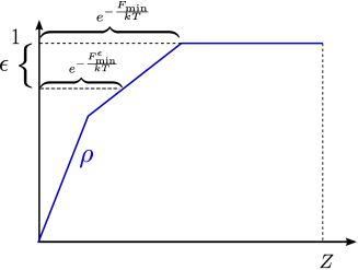
determined by the following smoothed version of $F_{\min}$

$$\begin{aligned} F_{\epsilon}^{\min}(\rho)=-kT\ln\sum h(\omega,\epsilon,g,E_{i})e^{-\beta E_{i}}\end{aligned}$$ (S59)

where $h(\omega,\epsilon,g,E_{i})=0$ for $i<l$, $h(\omega,\epsilon,g,E_{i})=\epsilon^{\prime}/p(E_{i})$ for $i=l$ and $h(\omega,\epsilon,g,E_{i})=1$ for $i>l$, with $\epsilon^{\prime}$ and $l$ determined using the method described above. We illustrate this in Supplementary Figure S2.

Supplementary Figure S2: Smoothing $F_{\min}$. Comparison of $F_{\min}$ and $F_{\epsilon}^{\min}$ for given failure probability $\epsilon$.

The above protocol clearly gives the maximal work for a given energy block. However, the maximal work is by definition a monotonic function of $\epsilon$, and the function does not depend on $E$, thus the maximal work for a given $\epsilon$ will be the same for the total state as for the block.

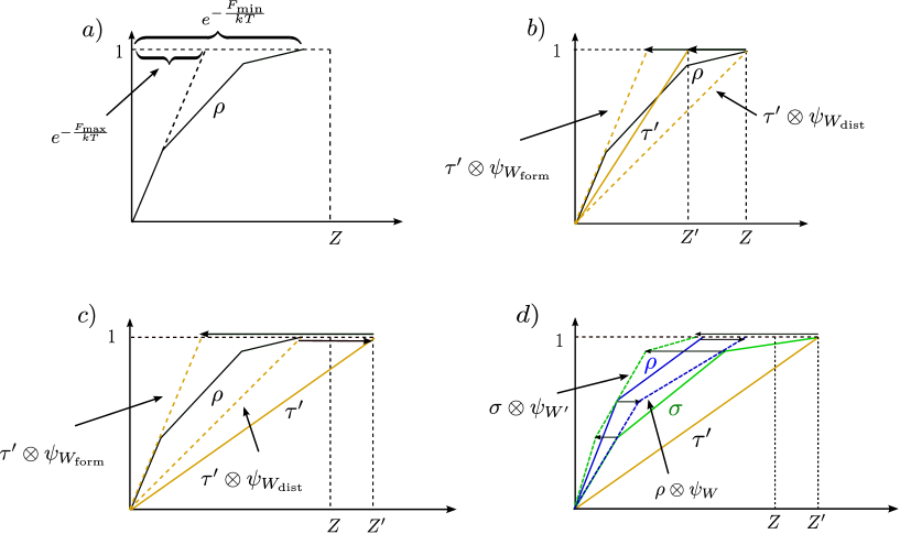
Now, let us pass to the formation process, provided we are allowed to produce a state $\rho^{\prime}$ which is $\epsilon$ close to the required state $\rho$ in trace norm. The amount of work needed is given by

$$\begin{aligned} W_{\epsilon}=F_{\epsilon}^{\max}(\rho)-F(\tau)\end{aligned}$$ (S60)

where

$$\begin{aligned} F_{\epsilon}^{\max}(\rho)=\min_{\rho^{\prime}}F_{\max}(\rho^{\prime})\end{aligned}$$ (S61)

where the minimum is taken over all $\rho^{\prime}$ satisfying $||\rho^{\prime}-\rho||\leq\epsilon$. Here we describe the algorithm to compute $F_{\epsilon}^{\max}$ for a given state (diagonal in the energy eigenbasis). Namely, one considers $\beta$-ordered eigenvalues of the state. In the first stage, one subtracts from the $\beta$-largest eigenvalue, and adds to the $\beta$-smallest one, until either the slope of a line corresponding to the $\beta$-largest on a thermo-majorization diagram (see Supplementary Figure S1d) will become equal to the slope of the second $\beta$-largest, or the slope of the $\beta$-smallest will become equal to the slope of the second $\beta$-smallest one. In the first case, the next step is to subtract from both eigenvalues, again, until their slope will become equal to the third $\beta$-largest eigenvalue, or until the slope of the $\beta$-smallest eigenvalue will become equal to the second $\beta$-smallest one. In the second case we proceed analogously. We continue, until the total amount of subtracted eigenvalue achieves $\epsilon$, or all slopes are equal. Note that the defined algorithm, when optimal ensures that we will not be left with some remaining part of $\epsilon$ at the end.

Supplementary Note 5 Catalytic transitions

So far we have considered the situation where the state $\rho$ describes all parts of the system of interest except for the heat bath $\tau$. However, we might want to consider $\rho$ to be a system of interest, interacting with an environment, ancillas, or working body that might be used, but should be returned in it’s original state. Such a process is called catalysis. In [41] we consider this issue in more detail, and here we mention how the results are related to the present findings. Let us recall, that the phenomenon of catalysis was discovered in entanglement theory, but it also directly translates into the theory of manipulations where purity (or negentropy) is a resource, where the allowed class of operations (called noisy operations) consist of (i) adding a system in maximally mixed state, (ii) arbitrary unitary transformations (iii) tracing out. Without using ancillas, the transitions are governed by majorization, i.e. we can transform probability distributions $p$ into $q$ if and only if $p$ majorizes $q$ (as in Eq. (S19))) which we denote by $p\succ q$. However, in [42] it was shown that some forbidden transitions can be possible, if we can use additional system as a catalyst, i.e. we may have $p\not\succ q$ but $p\otimes r\succ q\otimes r$ for some distribution $r$. One can then ask, what conditions should be satisfied by $p$ and $q$ such that an $r$ exists for which $p\otimes r\succ q\otimes r$. The conditions have been found in [47,48] and they are called trumping conditions. If we are allowed to obtain instead of $q$, an arbitrary good approximation of it, then the conditions are the following [41]

$$\begin{aligned} &&H_{\alpha}(p)\geq H_{\alpha}(q),\quad\text{for}\,\alpha\geq 0\\ &&H_{\alpha}(p)\leq H_{\alpha}(q),\quad\text{for}\,\alpha<0\end{aligned}$$

for $\alpha\in R$, where $H_{\alpha}$ is the Renyi entropy

$$\begin{aligned} H_{\alpha}(p)=\frac{1}{1-\alpha}\log\sum_{i}p_{i}^{\alpha}\end{aligned}$$ (S62)

with $H_{1}(p)=-\sum_{i}p_{i}\log p_{i}$, $H_{0}=\log\operatorname{rank}(p)$ where $\operatorname{rank}(p)$ is number of nonzero elements of $p$. Note that the original conditions are in the form of strict inequalities, however due to strict Schur concavity (convexity) of $H_{\alpha}$ for $\alpha>0$ ($\alpha<0$), one can change them into nonstrict ones. The above conditions determine possible catalytic transitions with trivial Hamiltonian. The conditions with negative $\alpha$ can be removed, if we are allowed to invest an arbitrarily small amount of work, or, equivalently, to borrow one pure qubit, and return it with arbitrary good fidelity.

Let us now turn to the case of a nontrivial Hamiltonian, which we consider in this paper. In [41] we prove, that the necessary and sufficient conditions are expressed in terms of Renyi divergences $D_{\alpha}(\rho|\tau)$ defined (for diagonal states) as

$$\begin{aligned} D_{\alpha}(\rho\|\sigma)=\frac{1}{\alpha-1}\log\sum_{i}p_{i}^{\alpha}q_{i}^{1-\alpha}\end{aligned}$$ (S63)

for $\alpha>0,\alpha\not=1$ where $p_{i}$, $q_{i}$ are the eigenvalues of $\rho$ and $\sigma$, respectively, and

$$\begin{aligned} D_{\alpha}(\rho\|\sigma)=\frac{1}{1-\alpha}\log\sum_{i}p_{i}^{\alpha}q_{i}^{1-\alpha}\end{aligned}$$ (S64)

for $\alpha<0$. For $\alpha=0,1$ we take $D_{1}(\rho|\sigma)=\sum_{i}p_{i}\log(p_{i}/q_{i})$ to be the standard relative entropy and $D_{0}(\rho|\sigma)=D_{\min}(\rho|\sigma)$ is the min-relative entropy. Now, for states block diagonal in the energy eigenbasis, $\rho$ can be catalytically transformed into an arbitrarily good approximation of $\rho^{\prime}$ by thermal operations, if and only if

$$\begin{aligned} D_{\alpha}(\rho\|\tau)\geq D_{\alpha}(\rho^{\prime}\|\tau)\end{aligned}$$ (S65)

for all $\alpha\in R$. Again, investing an arbitrarily small amount of work, one can remove the conditions with negative $\alpha$. Alternatively, conditions with negative $\alpha$’s are removed, when, exactly as in the case of the trivial Hamiltonian, one borrows one qubit in a pure state (with arbitrary Hamiltonian, which can be the trivial one) and returning it with arbitrary good fidelity. The conditions allow for some transitions that are not admitted by thermo-majorization. However, they do not affect the conditions for work of formation and distillation derived in this paper. Indeed, for the eigenstates of energy, the divergences with $\alpha\geq 0$ are all equal to the standard relative entropy. Moreover the Renyi divergence is increasing in $\alpha$ for $\alpha\geq 0$, so that, in particular, we have $D_{\min}\leq D_{\alpha}\leq D_{\max}$. Hence, in the case of distillation and formation, the conditions collapse to a single one: $D_{\min}$ and $D_{\max}$, respectively. Thus the effect of catalysis does not affect the thermo-majorization laws in this case. We note further that for $0<\alpha<2$ a quantum version of $D_{\alpha}(\rho\|\tau)$ is monotonically decreasing under CP maps [30], and in particular, under Thermal Operations, and thus for these values of $\alpha$, monotonicity of $D_{\alpha}(\rho\|\tau)$ provides a necessary condition for thermodynamic state transitions even for states which are not block diagonal in the energy eigenbasis.

If we allow the catalyst to be returned in a final state only close to its initial state, the crucial point is to choose correctly the distance measure, since for large systems, the standard distance (trace norm) allows the initial and final state of the catalyst to differ arbitrarily with respect to energy or entropy, thereby nullifying even the standard Second Law. In the theory of quantum resources this manifests itself via the phenomenon of embezzling - where one can perform arbitrary transformation, while returning a non-exact state with dimension large enough [49]. A natural condition that may be imposed, to avoid the phenomenon of embezzling is that it should be possible to obtain the required exact output from the approximate one (the one actually obtained) by investing some $\epsilon$ amount of work in addition. This implies the following (non-symmetric) distance we term the “trumping distance”

$$\begin{aligned} d(\rho\rangle\rho^{\prime})=\sup_{\alpha>0}(D_{\alpha}(\rho\|\tau)-D_{\alpha}(\rho^{\prime}\|\tau)).\end{aligned}$$ (S66)

In the smoothing procedure one should therefore use the above distance. This again does not change the conditions for smoothed work of formation and distillation. However, one can come up with other criteria, that interpolate between having no Second Law whatsoever, and the present limitations. The choice of criteria, that best fit the spirit of thermodynamics require further investigation.

Supplementary Note 6 Characterisation of Thermal Operations

We have provided an algorithm for deciding whether a state can be transformed into another state, given by thermo-majorization. However the algorithm does not tell us what kind of operations (completely positive maps) we can perform by means of Thermal Operations. Below we shall show, that all possible processes are precisely those that preserve the Gibbs state. This was shown for a special case of tensor product of i.i.d states [25]. Here, we show that it is true for a generic heat bath that satisfies our assumptions. This implies that if we have reversibility of state transformations (as is the case when we have many copies of a state [21], then the unique measure which determines whether a transformation is possible, is given by the relative entropy distance to the Gibbs state [28]. This quantity is the difference between free energy of a state of interest and that of the Gibbs state [19]. However, here, we do not have reversibility, thus there are at least two inequivalent functions which are non increasing under thermal operations ($F_{\min}$ and $F_{\max}$).

We start with a state $\tau_{R}\otimes\rho_{S}$ and write

$$\begin{aligned} \tau_{R}\otimes\rho_{S}\approx\sum_{E\in{\cal E}}p_{E}\rho_{RS}^{E}\end{aligned}$$ (S67)

with

$$\begin{aligned} \rho_{RS}^{E}=\frac{1}{P_{E}}P_{E}\tau_{R}\otimes\rho_{S}P_{E}\end{aligned}$$ (S68)

where ${\cal E}$ consists of very large energies in comparison with system energies, and $p_{E}=\mathop{\mathsf{tr}}\nolimits(\tau_{R}\otimes\rho_{S}P_{E})$. We shall now fix one energy block, and show, that even when restricting just to permutations of basis vectors within the block (being products of eigenstates of $\tau_{R}$ to eigenvalues $E_{R}$ and eigenstates of $\rho_{S}$ to eigenvalues $E_{S}$, such that $E_{R}+E_{S}=E$) we can perform arbitrary operation on system $S$ which preserve the Gibbs state. Then, we will argue that the operation on the system $S$ can be made the same for each energy block (for $E\in{\cal E}$).

To prove the first claim, for simplicity, let us assume that the Hamiltonian $H_{S}$ is nondegenerate (extension to the degenerate case is immediate). As follows from Theorem 2, in such a fixed subspace, the eigenvalues of our state form groups labelled by energy $E_{S}$. Within each group, we have $g_{R}(E)e^{-\beta E_{S}}$ eigenvalues all equal to $\frac{p(E_{S})}{g_{R}(E)e^{-\beta E_{S}}}$. Permutations of basis vectors result in transferring some subsets of a given group to other groups. Let us then use indices $i$ in place of $E_{S}$, so that $p_{E_{S}}\to p_{i}$ and $g_{R}(E)e^{-\beta E_{S}}\to d_{i}$. We shall denote by $k_{i\to j}$ the ”transition current” i.e. the number of eigenstates that have been moved from the $i$-th group to the $j-th$ group. Clearly $k_{i\to j}$ satisfy

$$\begin{aligned} \sum_{j}k_{i\to j}=d_{i}\\ \quad\sum_{i}k_{i\to j}=d_{j}\\ \end{aligned}$$ (S69)

The transition ”currents” are illustrated on Supplementary Figure S3.

Supplementary Figure S3: Transitions for two level system with energy levels $E=0$ and $E=1$. a) There are four possible transitions b) the number of states of bath corresponding to each level is proportional to the Boltzmann factor.

After an operation given by some fixed set of $k_{i\to j}$ satisfying the above transitions, we obtain a new state, whose probabilities $q_{i}$ are given by

$$\begin{aligned} q_{j}=\sum_{i}k_{i\to j}\frac{p_{i}}{d_{i}}\end{aligned}$$ (S70)

Thus, we can define transition probabilities $p_{i\to j}$ as

$$\begin{aligned} p_{i\to j}=\frac{k_{i\to j}}{d_{i}}\end{aligned}$$ (S71)

Then the condition (S69) means that the $p_{i\to j}$ ensure normalisation, so that the only constraint on possible process is (LABEL:eq:k2). However, since $\frac{d_{i}}{d_{j}}=\frac{e^{\beta E_{j}}}{e^{\beta E_{j}}}$, the latter condition means simply that the Gibbs state is preserved. This ends the proof, that for fixed $E$ we can perform all Gibbs preserving operations. Finally, given arbitrary Gibbs preserving transformation on $S$ we perform for every total energy block permutation that results in this transformation. In this way the needed transformation is performed on the initial state of system $S$. Of course, Thermal Operations obviously do preserve the Gibbs state, hence we obtain, that Thermal Operations are arbitrary operations that preserve the Gibbs state. Furthermore, although a single copy of another state (such as that of Equation 7) may also be preserved under Thermal Operations, if we allow many copies of some state, then only the Gibbs state is preserved. This follows immediately from the fact that the relative entropy distance to the Gibbs state is the unique monotone in the case of many copies of $\rho$ [21].

Let us discuss this result in the context of the detailed balance condition. The latter is the property that $\frac{p_{i\to j}}{p_{j\to i}}=e^{-\beta(E_{j}-E_{i})}$. As we will see, Thermal Operations need not satisfy detailed balance; they should merely preserve the Gibbs state as a whole. To provide an example, let us distinguish a class of Gibbs-preserving processes called quasi-cycles: we put the energy levels on a circle, and from one level, one can go only to the next neighbouring level, as in Supplementary Figure S4.

Supplementary Figure S4: Quasi-cycles. a) In the quasi cycle for each level there is only one transition to a different level b) a quasi-cycle for a three level system. The points represent levels with energies $0,1$ and $2$; probability $p_{2\to 2}$ of staying in level $2$ vanishes. c) Currents for a three-level quasi-cycle: the shaded microstates are subjected to a cycle, while the ones not shaded are left untouched.

The simplest description of a quasi-cycle is in terms of quantities $k_{i\to j}$. Namely, we choose an order of levels, put them on a circle, fix a direction, and the process is to take all states from the group of states with the largest energy $E_{S}$, and shift them to the states with the energy level in the chosen direction. I.e. the process is determined by $p_{i\to i+1}=e^{-\beta(E_{\max}-E_{i})}$, where $E_{\max}$ is the maximal energy, and $E_{i}$ is the energy of the $i$-th level.

For two level systems, the class of Gibbs preserving operations is the same as the class of operations satisfying the detailed balance condition, and all possible processes are parametrised by a single number $r\in[0,1]$, which is the probability of mixing two basic processes: the identity operation, and the two-level quasi-cycle. For three level systems, there are processes that preserve the Gibbs state, but do not satisfy detailed balance, an example being the three-level quasicycle. It turns out that the class of Gibbs preserving maps is strictly more powerful that the class of detailed-balance maps. An example is the transition between $(0,\frac{1}{2},\frac{1}{2})$ and $(\frac{1}{2}e^{-2\beta},\frac{1}{2}(1-e^{-}\beta),\frac{1}{2}(e^{-\beta}-e^{-2\beta}+1))$ with the energy levels given by $(0,1,2)$. It turns out that the only Gibbs preserving operation that can transform the first state into the second one is the quasi-cycle $0\to 1\to 2$. This means that such a transition is impossible by means of weak coupling with the heat-bath [50], as at weak coupling the detailed balance condition is satisfied.

Supplementary Note 7 Small engines undergoing a Carnot cycle

Here, we analyse a microscopic engine undergoing a Carnot cycle, between two heat reservoirs at temperatures $T_{H}$ and $T_{C}$ – see Supplementary Figure S5.

Supplementary Figure S5: Microscopic Carnot cycle. The double line for the isentropic processes illustrates different paths depending on whether the system is in the excited or ground state.

Since here, we are interested in work extraction from single systems, we are interested in how the engine behaves over a single cycle rather than its long term running efficiency. At stage $1$ the working body of the engine is in a thermal state, and is in contact with a thermal reservoir at temperature $T$. The Hamiltonian of the engine we call $H_{1}$ and we take the working body to be as small as possible - a qubit. If we were to then extract maximal work from the working body, we would do so at the rate given by Equation (3). However, the density matrix of the state of the working body, being thermal, has full rank and so, no work can be extracted without some probability of failure at least as large as it’s smallest eigenvalue, $e^{-\beta E_{\max}}/Z$. However, there is a way around this limitation – we can add a second system which is not in contact with the heat bath, and which acts as a switch qubit, as we did in Equation (10), and effectively change the Hamiltonian that acts on the working body from $H_{1}$ to $H_{2}$. The amount of work that can then be extracted in the first isothermal stage is then $W_{12}=-kT_{H}\ln{Z_{1}/Z_{2}}$ as given by Equation (13), and with $Z_{i}$ being the partition function corresponding to $H_{i}$. The work gained is stored in a work system $W$ which is initially in the ground state. We can thus perform the isothermal process reversibly and ideally, provided we add an extra system to simulate the changing Hamiltonian, and don’t extract the maximal amount of work from the engine.

Next we remove the working body from the thermal reservoir, and undergo the first adiabatic process. This will involve changing the Hamiltonian acting on the qubit slowly, so that the populations of the ground and excited state doesn’t change, and transferring the gained energy to our work system $W$. This requires that the switching system have a third state. At the end of this process (stage 3), the working body needs to be in a thermal state at temperature $T_{C}$ in order for the third stage to proceed reversibly. We thus need

$$e^{-\beta_{H}E_{2}^{e}}/Z_{2} =e^{-\beta_{C}E_{3}^{e}}/Z_{3}$$

$$e^{-\beta_{H}E_{2}^{g}}/Z_{2} =e^{-\beta_{C}E_{3}^{g}}/Z_{3}$$ (S72)

where $E_{i}^{g}$ and $E_{i}^{e}$ are the ground and excited energy levels of $H_{i}$.

Here we have a problem: we need to conserve energy, but the qubit of our working body could either be in the ground state or the excited state. To extract a deterministic amount of work, when we don’t know whether the working body is in the ground or excited state, we would need that the change in energy of the excited state, is the same as the change in energy of the ground state. i.e. that $W_{23}=E_{2}^{e}-E_{3}^{e}=E_{2}^{g}-E_{3}^{g}$. However, it is impossible to satisfy this condition, and those of Equations (S72). Either we need to return the qubit to the cold bath in a non-equilibrium state, resulting in inefficiencies, or we need to extract a different amount of work ($W_{23}^{e}=E_{2}^{e}-E_{3}^{e}$ and $W_{23}^{g}=E_{2}^{g}-E_{3}^{g}$), depending on whether the working body is in the ground or excited state. We therefore produce some additional entropy in the work system. In order to have the amount of entropy production be small compared with the amount of work extracted, one would need to have a larger heat engine – for example, if we have $n$ two level systems, we find the system has a higher probability to be around the average energy as $n$ increases, compared with being in the ground state [21], allowing us to conserve energy and more deterministically extract work.

Next, we perform the second isothermal stage, this time at temperature $T_{C}$. This time, the work is added to the system and is thus negative $W_{34}=-kT_{C}\ln{Z_{3}/Z_{4}}$ as given by Equation (13). Then we perform the final adiabatic process, and again, we have the same problem as before, extracting different amounts of work $W_{41}^{e}=E_{4}^{e}-E_{1}^{e}$ and $W_{41}^{g}=E_{4}^{g}-E_{1}^{g}$ depending on whether the engine qubit is in the ground or excited state. As before, we also want, that at the end of the final stage, the working body qubit is in equilibrium with $T_{H}$

$$e^{-\beta_{C}E_{4}^{e}}/Z_{4} =e^{-\beta_{H}E_{1}^{e}}/Z_{1}$$

$$e^{-\beta_{C}E_{4}^{g}}/Z_{4} =e^{-\beta_{H}E_{1}^{g}}/Z_{1}$$ (S73)

Solving Equations (S72)-(S73) we obtain Supplementary Table S1.

stage	1	2	3	4
$E^{e}$	$E$	$E_{2}^{e}=\frac{T_{H}}{T_{C}}E_{3}^{e}-\delta$	$E_{3}^{e}$	$E_{4}^{e}=\frac{T_{C}}{T_{H}}E+\delta^{\prime}$
$E^{g}$	$0$	$E_{2}^{g}=\frac{T_{H}}{T_{C}}-\delta$	$E_{3}^{g}$	$E_{4}^{g}=\delta^{\prime}$
$Z$	$Z_{1}=1+e^{-\beta_{H}E}$	$Z_{3}e^{\beta_{H}\delta}$	$Z_{3}=e^{-\beta_{C}E_{3}^{g}}+e^{-\beta_{C}E_{3}}$	$Z_{1}e^{-\beta_{H}E}$
$p_{e}$	$\frac{1}{Z_{1}}{e^{-\beta_{H}E}}$	$\frac{1}{Z_{3}}{e^{-\beta_{C}E_{3}}}$	$\frac{1}{Z_{3}}{e^{-\beta_{C}E_{3}}}$	$\frac{1}{Z_{1}}{e^{-\beta_{H}E}}$

Supplementary Table S1: Four stages of the Carnot cycle. $E^{e}$ and $E^{g}$ denote the excited and ground states of subsystem $S$ of the working body. The probability of being in the excited state is denoted by $p_{e}$.

At the end of a cycle, there are four possible amounts of work extracted, depending on whether the working body qubit was in the ground or excited state at stage $2$ and $4$. We label probabilities of those for events as $p_{ee},p_{eg},p_{ge},p_{gg}$. Regardless of what these probabilities are, it’s not hard to see that we obtain an amount of work that on average is equal to the amount obtained by an ideal engine

$$W_{avg} =-kT_{H}\ln{Z_{1}/Z_{2}}-(\frac{T_{H}}{T_{C}}-1)\langle E_{3}\rangle-\delta-kT_{C}\ln{Z_{3}/Z_{4}}-(\frac{T_{C}}{T_{H}}-1)\langle E_{1}\rangle+\delta^{\prime}$$

$$=(T_{H}-T_{C})(S_{B}-S_{A})$$ (S74)

However, in any single run of the cycle, we will see that there are three possible amounts of work which can be extracted, as depicted in Supplementary Table S2.

state	ee	eg	ge	gg
$\Delta W$	$(\frac{T_{H}}{T_{C}}-1)E_{3}^{e}+(\frac{T_{C}}{T_{H}}-1)E$	$(\frac{T_{H}}{T_{C}}-1)E_{3}^{e}$	$(\frac{T_{H}}{T_{C}}-1)E_{3}^{g}+(\frac{T_{C}}{T_{H}}-1)E$	$(\frac{T_{H}}{T_{C}}-1)E^{g}_{3}$
$\frac{e^{-\beta_{H}E}}{Z_{1}}\leq\frac{e^{-\beta_{C}E_{3}}}{Z_{3}}$	$p_{ee}=\frac{e^{-B_{H}E}}{Z_{1}}$	$p_{eg}=\frac{e^{-\beta_{C}E_{3}}}{Z_{3}}-\frac{e^{-\beta_{H}E}}{Z_{1}}$	$p_{ge}=0$	$p_{gg}=\frac{e^{-\beta E_{3}^{g}}}{Z_{3}}$
$\frac{e^{-\beta_{H}E}}{Z_{1}}\geq\frac{e^{-\beta_{C}E_{3}}}{Z_{3}}$	$p_{ee}=\frac{e^{-B_{C}E_{3}}}{Z_{3}}$	$p_{eg}=0$	$p_{ge}=\frac{e^{-\beta_{H}E}}{Z_{1}}-\frac{e^{-\beta_{C}E_{3}}}{Z_{3}}$	$p_{gg}=\frac{1}{Z_{1}}$

Supplementary Table S2: Work extracted in single Carnot cycle. Amount of work extracted in any single cycle depends on the state of the working body. There are four possible amounts of work extracted, depending on whether the working body qubit was in the ground or excited state at stage $2$ and $4$; we denote those events by ee, eg, ge and gg. Here, we only write the difference in the amount of work extracted compared with a basic amount of $W_{o}=-kT_{H}\ln{Z_{1}/Z_{3}}-kT_{C}\ln{Z_{3}/Z_{1}}$. There are two cases, one when $e^{-\beta_{H}E}/Z_{1}\leq e^{-\beta_{C}E_{3}}/Z_{3}$ and the other when $e^{-\beta_{H}E}/Z_{1}\geq e^{-\beta_{C}E_{3}}/Z_{3}$. In the first case, the entropy produced in a cycle is $S(W)=e^{-\beta_{H}E}/Z_{1}(\beta_{H}E+\ln{Z_{1}})+e^{-\beta_{C}E_{3}^{g}}/Z_{3}(\beta_{C}E_{3}^{g}+\ln{Z_{3}})-(e^{-\beta_{C}E_{3}}/Z_{3}-e^{-\beta_{H}E}/Z_{1})\ln{(e^{-\beta_{C}E_{3}}/Z_{3}-e^{-\beta_{H}E}/Z_{1})}$ and in the second case, $S(W)=\ln{Z_{1}}/Z_{1}+e^{-\beta_{C}E_{3}}/Z_{3}(\beta_{C}E_{3}+\ln{Z_{3}})+(e^{-\beta_{C}E_{3}}/Z_{3}-e^{-\beta_{H}E}/Z_{1})\ln{(e^{-\beta_{H}E}/Z_{1}-e^{-\beta_{C}E_{3}}/Z_{3})}$. The probabilities are computed under a process which minimises the probability that a transition between ground to excited or visa versa is undergone, which can be achieved under Thermal Operations.

The work storage system thus needs to be at least a four level system (initially in state $0$), and the engine is not ideal – entropy is pumped into the work storage system. Alternatively, one could remove the entropy by letting the higher energy states of the work system decay into the lowest level excited state.

Note that if we are interested in having the working body of our Carnot engine to be as small as possible, we can take

$$H_{2}=H_{4}$$ (S75)

so that the switching system need only be of dimension $3$. i.e. $2\times 3$ not including the work storage system of dimension $4$ per cycle. To approach the Carnot efficiency in a single cycle, might will need even more qubits. It would be interesting to compare our small Carnot type engine to the small versions [9,51,52] of the Brownian ratchet [53,54] when operating only a few cycles.

We thus see that small engines pump additional entropy into the system. In macroscopic systems, or the case of $\rho^{\otimes n}$ discussed in [21], the amount of entropy produced can be made arbitrarily small. Note that what is important is not that the spread in energy be small compared to the average energy (indeed, the Gibbs state $\tau^{\otimes n}$ has this property for $n$ large enough). Rather, we want that for a fixed average energy, the entropy of the work system needs to be arbitrarily small compared to the entropy of the corresponding heat bath at that average energy. However, here, this is not the case. If we wish to draw a deterministic amount of work, we sometimes fail, and we thus have a failure probability in micro-engines. Or rather than allowing a probability of failure, we could run the engine over many cycles, and then remove the additional entropy that was produced by acting collectively on the many work storage systems. However, here we are interested in the work produced by single systems, or during a single cycle, and thus, must be content to tolerate entropy production, an amount of work lower than the optimal amount, or a probability of failure.

References

- (1) Scovil, H. E. D. & Schulz-DuBois, E. O. Three-level masers as heat engines. Phys. Rev. Lett. 2, 262–263 (1959). http://link.aps.org/doi/10.1103/PhysRevLett.2.262
- (2) Geusic, J. E., Schulz-DuBios, E. O. & Scovil, H. E. D. Quantum equivalent of the carnot cycle. Phys. Rev. 156, 343–351 (1967). http://link.aps.org/doi/10.1103/PhysRev.156.343
- (3) Alicki, R. The quantum open system as a model of the heat engine. J. Phys. A: Math. Gen. 12, L103–L107 (1979).
- (4) Howard, J. Molecular motors: structural adaptations to cellular functions. Nature 389, 561–567 (1997).
- (5) Geva, E. & Kosloff, R. On the classical limit of quantum thermodynamics in finite time. J. Chem. Phys. 97, 4398 (1992).
- (6) Hänggi, P. & Marchesoni, F. Artificial brownian motors: Controlling transport on the nanoscale. Rev. Mod. Phys. 81, 387–442 (2009). http://link.aps.org/doi/10.1103/RevModPhys.81.387
- (7) Allahverdyan, A. E. & Nieuwenhuizen, T. M. Extraction of work from a single thermal bath in the quantum regime. Phys. Rev. Lett. 85, 1799–1802 (2000). http://link.aps.org/doi/10.1103/PhysRevLett.85.1799
- (8) Feldmann, T. & Kosloff, R. Quantum lubrication: Suppression of friction in a first-principles four-stroke heat engine. Phys. Rev. E 73, 025107 (2006). http://link.aps.org/doi/10.1103/PhysRevE.73.025107
- (9) Linden, N., Popescu, S. & Skrzypczyk, P. How small can thermal machines be? the smallest possible refrigerator. Phys. Rev. Lett. 105, 130401 (2010).
- (10) Scully, M. O. Quantum afterburner: Improving the efficiency of an ideal heat engine. Phys. Rev. Lett. 88, 050602 (2002). http://link.aps.org/doi/10.1103/PhysRevLett.88.050602
- (11) Rousselet, J., Salome, L., Ajdari, A. & Prost, J. Directional motion of brownian particles induced by a periodic asymmetric potential. Nature 370, 446–447 (1994).
- (12) Faucheux, L. P., Bourdieu, L. S., Kaplan, P. D. & Libchaber, A. J. Optical thermal ratchet. Phys. Rev. Lett. 74, 1504–1507 (1995). http://link.aps.org/doi/10.1103/PhysRevLett.74.1504
- (13) Landauer, R. IBM J. Res. Develop. 5, 183 (1961).
- (14) Bennett, C. H. The thermodynamics of computation-a review. Int. J. Theor. Phys. 21, 905–940 (1982).
- (15) Baugh, J., Moussa, O., Ryan, C., Nayak, A. & Laflamme, R. Experimental implementation of heat-bath algorithmic cooling using solid-state nuclear magnetic resonance. Nature 438, 470–473 (2005).
- (16) Gemmer, J., Michel, M., Michel, M. & Mahler, G. Quantum thermodynamics: Emergence of thermodynamic behavior within composite quantum systems (Springer Verlag, 2009).
- (17) Popescu, S., Short, A. & Winter, A. Entanglement and the foundations of statistical mechanics. Nat. Phys. 2, 754–758 (2006).
- (18) Del Rio, L., Åberg, J., Renner, R., Dahlsten, O. & Vedral, V. The thermodynamic meaning of negative entropy. Nature 474, 61–63 (2011).
- (19) Donald, M. J. Free energy and the relative entropy. J. Stat. Phys. 49, 81–87 (1987).
- (20) Esposito, M. & den Broeck, C. V. Second law and landauer principle far from equilibrium. Euro Phys. Lett. 95, 40004 (2011).
- (21) Brandão, F., Horodecki, M., Oppenheim, J., Rennes, J. & Spekkens, R. The resource theory of quantum states out of thermal equilibrium (2011). Preprint at http://arxiv.org/abs/arXiv:1111.3812.
- (22) Horodecki, M., Horodecki, P. & Oppenheim, J. Reversible transformations from pure to mixed states and the unique measure of information. Phys. Rev. A 67, 062104 (2003). Preprint at http://arxiv.org/abs/quant-ph/0212019.
- (23) Dahlsten, O., Renner, R., Rieper, E. & Vedral, V. Inadequacy of von neumann entropy for characterizing extractable work. New J. Phys. 13, 053015 (2011).
- (24) Gour, G. & Spekkens, R. W. The resource theory of quantum reference frames: manipulations and monotones. New J. Phys. 10, 033023 (2008).
- (25) Janzing, D., Wocjan, P., Zeier, R., Geiss, R. & Beth, T. Thermodynamic cost of reliability and low temperatures: Tightening Landauer’s principle and the second law. Int. J. Theor. Phys. 39, 2717–2753 (2000). Preprint at http://arxiv.org/abs/quant-ph/0002048.
- (26) Werner, R. F. Quantum states with einstein-podolsky-rosen correlations admitting a hidden-variable model. Phys. Rev. A 40, 4277–4281 (1989).
- (27) Bennett, C. H., DiVincenzo, D. P., Smolin, J. A. & Wootters, W. K. Mixed-state entanglement and quantum error correction. Phys. Rev. A 54, 3824–3851 (1996). Preprint at http://arxiv.org/abs/quant-ph/9604024.
- (28) Horodecki, M., Oppenheim, J. & Horodecki, R. Are the laws of entanglement theory thermodynamical? Phys. Rev. Lett. 89, 240403 (2002). Preprint at http://arxiv.org/abs/quant-ph/0207177.
- (29) Tomamichel, M. A framework for non-asymptotic quantum information theory (2012). Preprint at http://arxiv.org/abs/arXiv:1203.2142.
- (30) Datta, N. Min-and max-relative entropies and a new entanglement monotone. IEEE Trans. Inf. Theory 55, 2816–2826 (2009).
- (31) Åberg, J. Truly work-like work extraction (2011). Preprint at http://arxiv.org/abs/arXiv:1110.6121.
- (32) Renner, R. Security of quantum key distribution (2005). PhD. thesis, ETH, Preprint at http://arxiv.org/abs/quant-ph/0512258.
- (33) Ruch, E. The diagram lattice as structural principle a. new aspects for representations and group algebra of the symmetric group b. definition of classification character, mixing character, statistical order, statistical disorder; a general principle for the time evolution of irreversible processes. Theoretical Chemistry Accounts: Theory, Computation, and Modeling (Theoretica Chimica Acta) 38, 167–183 (1975).
- (34) Ruch, E. & Mead, A. The principle of increasing mixing character and some of its consequences. Theoretical Chemistry Accounts: Theory, Computation, and Modeling (Theoretica Chimica Acta) 41, 95–117 (1976).
- (35) Ruch, E., Schranner, R. & Seligman, T. H. The mixing distance. J. Chem. Phys. 69, 386–392 (1978).
- (36) Janzing, D., Wocjan, P., Zeier, R., Geiss, R. & Beth, T. Thermodynamic cost of reliability and low temperatures: Tightening landauer’s principle and the second law. Int. J. Theor. Phys. 39, 2717–2753 (2000).
- (37) Petz, D. Quasi-entropies for finite quantum systems. Rep. Math. Phys. 23, 57 (1986).
- (38) Brandão, F. G. & Plenio, M. B. A reversible theory of entanglement and its relation to the second law. Nat. Phys. 4, 873 (2008). Preprint at http://arxiv.org/abs/arXiv:0710.5827.
- (39) Bennett, C. H., Bernstein, H. J., Popescu, S. & Schumacher, B. Concentrating partial entanglement by local operations. Phys. Rev. A 53, 2046 2052 (1996). Preprint at http://arxiv.org/abs/quant-ph/9511030.
- (40) Marvian, I. & Spekkens, R. W. Pure state asymmetry (2011). Preprint at http://arxiv.org/abs/1105.1816.
- (41) Brandão, F. G. S. L., Horodecki, M., Huei Ying Ng, N., Oppenheim, J. & Wehner, S. The second laws of quantum thermodynamics, Preprint at http://arxiv.org/abs/1305.5278.
- (42) Jonathan, D. & Plenio, M. B. Entanglement-assisted local manipulation of pure quantum states. Phys. Rev. Lett. 83, 3566 3569 (1999).
- (43) Oppenheim, J. Non-extensive thermodynamics: from Ising models to black-holes. Phys. Rev. E 68, 016108 (2003). Preprint at http://arxiv.org/abs/gr-qc/0212066.
- (44) Oi, D. & Oppenheim, J. Equilibrium temperature anisotropy and black-hole analogues. Preprint at http://arxiv.org/abs/grqc/ 0702010.
- (45) Hartmann, M., Mahler, G. & Hess, O. Existence of temperature on the nanoscale. Phys. Rev. Lett. 93, 80402 (2004).
- (46) Uhlmann, A. Wiss Z. Karl-Marx-Univ. Leipzig 20, 633 (1971).
- (47) Klimesh, M. Inequalities that Collectively Completely Characterize the Catalytic Majorization Relation (2007). Preprint at http://arxiv.org/abs/0709.3680.
- (48) Turgut, S. Catalytic transformations for bipartite pure states. J. Phys. A, Math. Gen. 40, 12185 12212 (2007). Preprint at http://arxiv.org/abs/0707.0444.
- (49) van Dam, W. & Hayden, P. Universal entanglement transformations without communication. Phys. Rev. A 67, 060302 (2003). Preprint at http://arxiv.org/abs/quant-ph/0201041.
- (50) Alicki, R. & Lendi, L. Quantum dynamical semigroups and applications (Springer, 1993).
- (51) Brunner, N., Popsecu, S., Linden, N. & Skrzypczyk, P. Virtual qubits, virtual temperatures, and the foundations of thermodynamics Preprint at http://arxiv.org/abs/1106.2138.
- (52) Skrzypczyk, P., Linden, N., Brunner, N. & Popescu, S. On the efficiency of very small refrigerators. J Phys A Math Theor 44, 492002 (2011).
- (53) von Smoluchowski, M. Experimentell nachweisbare, der ublichen thermodynamik widersprechende molekularphanomene. Physik. Zeitschr. XIII, 1069 1080 (1912).
- (54) R.P. Feynman, R. L. & Sands, M. The Feynman Lectures on Physics, vol. 1 (Addison-Wesley, 1963).