An Experimental Investigation of SIMO, MIMO, Interference-Alignment (IA) and Coordinated Multi-Point (CoMP)

Abstract

In this paper we present experimental implementations of interference alignment (IA) and coordinated multi-point transmission (CoMP). We provide results for a system with three base-stations and three mobile-stations all having two antennas. We further employ OFDM modulation, with high-order constellations, and measure many positions both line-of-sight and non-line-of-sight under interference limited conditions. We find the CoMP system to perform better than IA at the cost of a higher back-haul capacity requirement. During the measurements we also logged the channel estimates for off-line processing. We use these channel estimates to calculate the performance under ideal conditions. The performance estimates obtained this way is substantially higher than what is actually observed in the end-to-end transmissions—in particular in the CoMP case where the theoretical performance is very high. We find the reason for this discrepancy to be the impact of dirty-RF effects such as phase-noise and non-linearities. We are able to model the dirty-RF effects to some extent. These models can be used to simulate more complex systems and still account for the dirty-RF effects (e.g., systems with tens of mobiles and base-stations). Both IA and CoMP perform better than reference implementations of single-user SIMO and MIMO in our measurements.

Index Terms—  Interference alignment (IA), coordinated multipoint (CoMP), testbed, wireless, MIMO, SIMO, USRP.

1 Introduction

Interference alignment (IA) is a concept that was introduced in the seminal paper [1]. The wording “interference” and “alignment” refers to the fact that according to the strategy, the interfering signals should be confined to a subspace disjoint from the subspace of the desired signals, - when transmitting over MIMO channels. This MIMO channel may result from using multiple-antennas or using so-called symbol extended channels (e.g., using multiple carriers). However, in this paper we will only consider the case of MIMO channels achieved using multiple antennas.

In order to investigate the usefulness of IA in practice, we are herein analyzing the results of a real-world implementation of IA. Experimentation with IA was pioneered in [2, 3] and [4]. In the paper [2] considers a variant of IA with co-operation also among the receivers. This is different from the scenario herein and will not be discussed further. The paper [5] simulations using measured channels is performed. In this paper we are concerned with the difference between the performance calculated in this manner and the results that are observed when actually transmitting over the channel. The paper [4] does transmit over actual channels. Moreover, [4] also presents end-to-end error-vector measurements (EVM) which is a very relevant representation of the quality of the end-to-end channel, including the impact of real-world hardware such as non-linearities, phase-noise, and inter-symbol interference. The EVM quantifies the quality of the transmission channel seen from the view-point of the modulator and de-modulator which operate over the virtual SISO channels created by transmit beamformers and receive combiners.

This paper uses an OFDM modulation with higher bandwidth and higher modulation order than [4] does. We further include a high-performance LDPC code and reduce the time between frames from five seconds used in [4] to a tenth of a second. In addition, we also consider several positions of the mobile-stations including many non line-of-sight positions thus exposing IA to a more diverse set of channels.

Parallel to the development of IA, the concept of coordinated multi-point transmission (CoMP) has also emerged with interest from 3GPP standardization. This approach is similar to IA but assumes that the signals from multiple base-stations have a common phase-reference and that all base-stations know the information to be transmitted to every mobile-station which is not the case in IA. However, both IA and CoMP require information about the channel between all transmitting base-stations and all receiving mobile-stations.

Pioneering experimentation with CoMP is found in [6, 7, 8]. The paper [6] presented the performance from trials using a setup with two LTE base- and mobile-stations. Solutions for acquiring the necessary channel state information at the base- and mobile-stations are described. The paper [7] presents similar measurements. While the papers [6] and [7] present absolute (impressive) numbers of throughput the papers lack any specific comparison between the measurements results and theory. The paper [8] looks into the difference between “estimated” and “measured” SINR, but provides very little detail on their analysis.

In this paper we also implement a form of CoMP. We compare it with IA and with the well-known base-line schemes of single-user SIMO and MIMO. We further use three base-stations and mobile-stations while the above cited papers use two.

Most importantly, we provided a detailed analysis of the difference between performance that would have been obtained when performing a typical simulation of the scenario at hand and the performance actually obtained. This difference (“the delta”) can be used to extrapolate the real-world performance in more complex scenarios and provide useful insight into the factors that come into play in the real world.

2 Testbed Setup

Our testbed consists of six nodes, of which three take the role of base-stations and three take the role of mobile-stations. We consider the downlink but one could also interpret the results as uplink although it is less natural. All nodes have two vertically polarized dipole antennas spaced 20cm apart or 1.6 wavelengths at our 2490MHz carrier frequency. This carrier frequency is unoccupied in the building where the measurements were conducted. The base-station transmitters consist of USRP N210 motherboards with XVRC2450 daughterboards, see www.ettus.com. The output signal is connected to a ZRL-2400LN amplifier to obtain a +15dBm output power with good linearity. The receivers consist of custom boards assembled by using amplifiers, filters and mixers from mini-circuits, see www.minicircuits.com. The receiver noise figure is around 10-11dB. During measurements very close to the base-stations an additional 10dB attenuator was inserted between the antennas and the receiver boards in order to avoid saturation. The boards were tuned using attenuators to make the noise variance approach a nominal value $\sigma^{2}_{\text{nominal}}$. The actual noise variance varies up to one decibel from $\sigma^{2}_{\text{nominal}}$. The value $\sigma^{2}_{\text{nominal}}$ is known by all nodes. The analog output signal from the receiver boards are digitized at an intermediate frequency of 70MHz by USRP N210/2 boards equipped with basic daughterboards. A photograph of a receiver-node is shown in Fig. 1. The sample-clocks of all six nodes are locked to a common 10MHz reference and a common one pulse-per-second clock using long cables. This simplifies the implementation and gives a synchronization similar to that of a e.g. an LTE system where all mobile-stations derive the timing from common control channels. However, the oscillators of the three receiver nodes in our system are not locked to the reference and thus there are small frequency offsets and resulting phase rotations among the three receiver nodes and the transmitters. The base-band processing and system control is implemented on two PCs, one for all the base-station nodes and one for all the mobile-station nodes (the USRPs are connected with long Ethernet cables to the PCs, each having seven Ethernet connections in all). The processing for each node runs in a separate thread. The feedback from the mobile-station PC to the base-station PC is achieved with an Ethernet cable between the two PCs.

\psfrag{u2}[b][b][0.5]{signal generator}\psfrag{a}[b][b][0.5]{antennas}\psfrag{u}[b][b][0.5]{USRP}\psfrag{r}[b][b][0.5]{Receiver modules}\psfrag{d}[t][b][0.5]{Local oscillator generator}\psfrag{v}[b][t][0.5]{DC generator}\psfrag{s}[l][bl][0.5]{Cables (10MHz, PPS, Ethernet, power)}\includegraphics[width=202.58052pt,height=162.89201pt]{setup1.eps}

Fig. 1: A receiver node

3 Air Interface and Signal Processing

The air interface is based on an OFDM modulation with 38 subcarriers, with 312.5kHz subcarrier spacing and a cyclic prefix of 0.48$\mu$s. The modulation applied on each subcarrier is 16QAM. The data is encoded in blocks of 1140 bits with a rate of 0.75 using an LDPC code. Two coding blocks are transmitted per frame. The frame-structure is indicated in Fig. 2. During the time indicated as “payload”, modulated symbol streams are transmitted from all base-stations using individual precoders (i.e., beamformers). In the section marked “demodulation reference pilots”, all subcarriers are occupied by known reference symbols which have been processed by the same precoder as the corresponding stream. The demodulation reference pilots are transmitted for one stream at a time thereby avoiding any interference. In the area marked ”CSI”, channel state information pilots are transmitted. This means that a pilot symbol is transmitted from each of the six antennas in the system sequentially without interference. The mobile-stations estimate their channels independently for each subcarrier and feed back the impulse responses to one of the base-stations which then has “global” channel state information. This (master) base-station calculates the beamformers and informs the other base-stations of the result. The beamformers are calculated according to the “max-SINR” approach described in [9]. The total power of all streams is normalized to +15dBm. This approach is followed both in the IA and CoMP cases. The difference being that all streams emanate from a single six-antenna base-station in the CoMP case and three distinct two-antenna base-stations in the IA case.

\psfrag{0}[b][b][0.5]{$0$}\psfrag{1}[b][b][0.5]{$1$}\psfrag{9}[b][bl][0.5]{$9$}\psfrag{10}[b][bl][0.5]{$10$}\psfrag{11}[b][bl][0.5]{$11$}\psfrag{19}[b][bl][0.5]{$19$}\psfrag{5}[b][bl][0.5]{$5$}\psfrag{n}[b][b][0.5][90]{$n_{\text{s}}-1$}\psfrag{p1}[b][b][0.5]{Payload data}\psfrag{p2}[b][b][0.5]{Payload data}\psfrag{d}[b][b][0.5]{Demodulation pilots}\psfrag{c}[b][b][0.5]{CSI pilots}\includegraphics[width=202.58052pt,height=65.16078pt]{frame.eps}

Fig. 2: The frame-structure

The master base-station calculates a receiving vector (combiner) for each mobile-station. This vector is not used by the receiver. Instead the receiver uses an MMSE vector calculated based on the demodulation pilot symbols of the desired and interfering streams and the nominal noise power.

The overhead of the CSI pilots is substantial. However, the frame is only 0.1ms long. The payload of the frame could be made much longer without the need for additional pilots (assuming moderate mobility) - and thereby reduce the overhead in relative terms. For this reason we will ignore the overheads when calculating throughput.

In the reference cases SIMO and MIMO, - no closed-form beamforming is used. In fact, no beamforming is used at all. The SIMO and MIMO cases exist in two variants “TDMA” and “All-ON”. In the TDMA case only one base-station is transmitting at a time while all base-stations are active all the time in the All-ON mode. Thus the total number of streams in the system is one in the TDMA-SIMO case, two in the TDMA-MIMO case, three in the All-SIMO case and six in the All-MIMO case. In the IA and CoMP cases, there are three streams in the system. This is the maximum number of streams for IA - while CoMP could utilize more and thereby potentially improve performance.

4 Measurement Campaign

The measurements were made in 116 batches. In each batch, all the schemes were run sequentially with one second delay between the schemes. Each scheme was run with five frames inter-spaced 0.1seconds. The statistics from the first of these five frames is not used since the base-stations have not yet received any feedback information from the mobile-stations. The personnel involved in the measurements were standing still during the batches in order not to outdate the channel state information at the transmitter and give all schemes as similar channels as possible.

The measurement environment can be classified as indoor office, see Fig. 3. The three base-stations were distributed as shown in the floor-map of Fig. 4. The power of the base-stations were 15dBm . The three mobile-stations were fixed during the batches but moved moved between the batches. The mobile-stations were mostly located within the circle sorrounding it’s associated base-station in Fig. 4.

\psfrag{ta}[l][b][0.5]{Transmitter antennas of BS \#1}\psfrag{ms1}[l][b][0.5]{Mobile-station \#1}\psfrag{ms2}[b][b][0.5]{Mobile-station \#2}\psfrag{bs2}[b][b][0.5]{Base-station \#2}\psfrag{bs1}[b][b][0.5]{Base-station \#1}\includegraphics[width=202.58052pt,height=110.76538pt]{setup2.eps}

Fig. 3: The measurement environment and some equipment

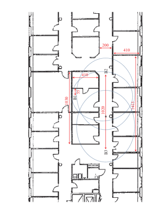
Fig. 4: Map of the measurement environment. The positions of the base-stations are marked BS1, BS2 and BS3. The three circles indicate the areas within which MS1, MS2 and MS3 roamed around during the measurements.

5 Results

In this section we present the measurement results from the described in the previous section. We first note that the raw signal to thermal noise ratio (i.e. without any spatial processing and averaged over all subcarriers) was in the range of 32dB to 61dB. Thus the thermal noise is almost negligable.

5.1 Raw Results

The transmitted data is generated from a random number generator - the seed of which is calculated from the start time of the batch. The mobile-stations are thus able to calculate the bit and frame-error rates (FER). The frame error rate is listed for all the implemented schemes in Table 1. The reader may note that CoMP is performing significantly better than IA in the part of the table under “All data”. In this part of the data the mobile-station may not be connected to the strongest base-station. Thus a substantial performance improvement can be achieved by simply handing over the mobile-station to the strongest base-station. In order to clean the results from this effect, the results in Table 1 are divided into two parts: one where all batches are used and one where only data for mobile-stations connected to the strongest base-station are used.All the remaining results will consider the “Best-BS” case.

In Table 1 we have also plotted the throughput defined as $n_{\text{s}}(1-\text{FER})$ where $n_{\text{s}}$ is the number of streams in the system.

	All data		Best BS
Method	FER	c-FER	FER	c-FER	rate	c-rate
IA	0.31	0.04	0.21	0.02	2.36	2.95
CoMP	0.01	0.00	0.06	0.01	2.81	2.97
TDMA-MIMO	0.08	0.01	0.04	0.00	1.93	2.00
TDMA-SIMO	0.00	0.00	0.00	0.00	1.00	1.00
All-MIMO	0.99	0.92	0.98	0.87	0.13	0.78
All-SIMO	0.76	0.55	0.61	0.31	1.18	2.07

Table 1: FER: Raw frame error rate, c-FER: frame error rate of coded bits, rate: average number of correct frames times the number of streams, c-rate: as rate but with coded bits, All-data: all batches are used, Best-BS only batches where the MS is connected to the strongest BS.

From Table 1 we conclude that the performance of CoMP is better than IA for uncoded transmissions. For coded transmissions both IA and CoMP exhibit a FER very near zero. The reference schemes SIMO and MIMO are all worse than IA and CoMP, - and reach only 70% of their rate.

5.2 Comparison: Measurements against Theory

An important aspect of experimentation is to verify the models used for system simulations. This is important since we are unable to experimentally investigate every relevant scenario - of propagation environment, user distribution, traffic loads, algorithm parameters and so on. Therefore we focus on quantifying the difference between the performance we would have predicted for the scenario at hand and the performance we actually obtained. The result of this analysis in illustrated in Fig. 5, 6 and 7 for the IA, COMP and TDMA-SIMO cases, respectively. The details of this analysis is described below.

5.2.1 EVM and Performance Modelling

We start-off with the performance that may be predicted given the measurements from the CSI pilots only. Based on these measurements we calculate the beamforming vectors of our beamforming strategy according to [9] and obtain “post-processed” signal to interference and noise ratios (SINR-post) at the output of the receiver combining (i.e., the quality of the equvivalent SISO channels formed by transmit beamformer and receive combiners).The SINR-post factor is finally obtained as an average over the subcarriers calculated as

$$\text{SINR-post}=\frac{\sum_{i}S_{i}}{\sum_{i}I_{i}+\sigma^{2}_{\text{nominal}}},$$ (1)

where $S_{i}$,$I_{i}$ and $\sigma^{2}_{\text{nominal}}$ are the signal, interference and nominal noise power on the $i$th subcarrier in a certain frame (the noise power is assumed identical on all subcarriers). The CDF of the resulting SINR-post is plotted in Fig. 5-7 and is marked with the legend “ideal”. The above calculation neglected the channel estimation errors and the fact that the channel may change between frames. In other words, it is non-causal as the channel state information used in the calculation of the beamformers is actually not available until after the time the frame has been transmitted. As a next step we therefore replace the channel state used in the transmit beamformers with channel state available in the previous frame. The result is also shown in Fig. 5-7 and marked with “causal”. Is this the real quality of the channel as seen by the mobile-station? - no it’s not. The real quality of the channel seen from the view-point of the SISO modem (which is transmitting over the equivalent SISO channel created by transmitter precoding and receiver combining) is best represented by the error vector magnitude. The error vector is defined as the difference between the receive constellation points and the true constellation points as illustrated in Fig. 8. The error vector magnitude is defined as root of the variance of the error vector, normalized by the power of the constellation positions. To compare this value with the previously calculated SINR values we form the following EVM based SINDR estimate

$$\text{SINDR}_{\text{EVM}}=\sum_{i}p_{i}\text{EVM}_{i}^{-2},$$ (2)

where $p_{i}$ is the power of the virtual SISO channel on subcarrier $i$ and $\text{EVM}_{i}$ is the EVM of the corresponding subcarrier. We use this power-weighted EVM value as it corresponds better to the average SINR value defined in (1) than a straight average. Note that we have used the acronym SINDR in (2). This acronym denotes “signal to noise, interference and distortion ratio” in order to emphasize that the $\text{SINDR}_{\text{EVM}}$ measure will include also the dirty-RF impairments caused by phase-noise and non-linearities i.e. the “distortions”.

The curves labelled “EVM-model” in Fig. 5-7 are obtained by using the same non-causal channel matrices as “ideal”. However, this model includes also the error model used in [10] and a common phase error. In [10] a Gaussian noise term is added to each transmitter and receiver antenna branch. The power of this modeled noise is set to 34dB below the desired signal in the transmitter and 40dB below in the receiver. These values have been estimated from the SISO measurements and from the data-sheet of the MAX2829 circuit, http://www.maxim-ic.com/datasheet/index.mvp/id/4532, used in the XCVR2450 daughterboard. Note that this error will affect both the payload symbols and the training. In addition to the model of [10] we also introduce a so-called common phase rotation, see [11]. This is a phase-error which (despite it’s name) will be independent between all our six transmitter branches (since each has its own local oscillator). This phase error will be introduced as a random rotation of the phase of the six transmitter branches which is re-randomized between frames. The phase is set to Gaussian with standard deviation of 0.6 degrees, again based on the data-sheet of the MAX2820 circuit.

5.2.2 Discussion

From Fig. 5-7 we conclude that our EVM-model is able to bridge most of the gap between the “ideal” and “EVM model” results. This indicates that most of the degradation between the “ideal” and “causal” curves are not due to the propagation channel evolution during the consecutive time-slots but due to dirty-RF effects. However, there is still some difference between the “EVM model” and the actual EVM measurements. Part of this difference could be due to channel evolution, but not all of it. Since there is also a mismatch in the SIMO case. A detailed studied of the actual performance of the hardware could help reducing the gap further.

Finally, we ask the reader to notice the extremely high performance of the CoMP scheme in the “ideal” case (far superior over the IA “ideal” case) . However, this performance advantage diminishes into a more modest advantage in reality. This implies that CoMP is very susceptible to any kind of non-idealness. Sensitivity of CoMP to common phase rotation was also recently studied in [12].

\psfrag{a}[lt][r][0.5]{$\text{SINR-post}$ ideal}\psfrag{b}[lt][r][0.5]{$\text{SINR-post}$ causal}\psfrag{c}[lt][r][0.5]{$\text{SINDR}_{\text{EVM}}$ measured}\psfrag{d}[lt][r][0.5]{$\text{SINDR}_{\text{EVM}}$ model}\includegraphics[width=202.58052pt,height=162.89201pt]{SINDR_IA.eps}

Fig. 5: Interference-alignment: Distribution of signal to interference, noise, and distortion ratio (SINDR) based on different models and measurements

\psfrag{a}[lt][r][0.5]{$\text{SINR-post}$ ideal}\psfrag{b}[lt][r][0.5]{$\text{SINR-post}$ causal}\psfrag{c}[lt][r][0.5]{$\text{SINDR}_{\text{EVM}}$ measured}\psfrag{d}[lt][r][0.5]{$\text{SINDR}_{\text{EVM}}$ model}\includegraphics[width=202.58052pt,height=162.89201pt]{SINDR_COMP.eps}

Fig. 6: Coordinated Multi-Point: Distribution of signal to interference, noise, and distortion ratio (SINDR) based on different models and measurements

\psfrag{a}[lt][r][0.5]{$\text{SINR-post}$ ideal}\psfrag{b}[lt][r][0.5]{$\text{SINR-post}$ causal}\psfrag{c}[lt][r][0.5]{$\text{SINDR}_{\text{EVM}}$ measured}\psfrag{d}[lt][r][0.5]{$\text{SINDR}_{\text{EVM}}$ model}\includegraphics[width=202.58052pt,height=162.89201pt]{SINDR_SIMO.eps}

Fig. 7: TDMA SIMO: Distribution of signal to interference, noise, and distortion ratio (SINDR) based on different models and measurements

Fig. 8: Illustration of error vector

6 Conclusions

We have implemented interference alignment (IA) and coordinated multi-point (CoMP) on a wireless testbed. We observe an performance improvement over reference schemes such as SIMO and MIMO. However, the gains are much smaller than what could be theoretically calculated on the basis from our channel estimates. The reason being that dirty-RF effects come into play and substantially degrade the performance. We are able to model the dirty-RF effects reasonably well with simple models but there is still room for improvement. The performance of CoMP is the highest of the implemented schemes. However, the performance advantage is not as great as predicted by theory. Both CoMP and IA perform better than the reference schemes of single-user SIMO and MIMO.

References

- [1] V.R. Cadambe and S.A. Jafar, “Interference alignment and degrees of freedom of the k -user interference channel,” IEEE Transactions on Information Theory, vol. 54, no. 8, pp. 3425 –3441, aug. 2008.
- [2] S. Gollakota, S.D. Perli, and D. Katabi, “Interference alignment and cancellation,” in the ACM Conference on Data Communication (SIGCOMM ’09), August 2009, pp. 159–170.
- [3] O. El Ayach, S.W Peters, and R.W Heath, “The feasibility of interference alignment over measured mimo-ofdm channels,” IEEE Transactions on Vehicular Technology, vol. 59, no. 9, pp. 4309 –4321, nov. 2010.
- [4] Ó. González, D. Ramírez, I. Santamaria, J.A. Garcí́a-Naya, and L. Castedo, “Experimental validation of interference alignment techniques using a multiuser mimo testbed,” in Smart Antennas (WSA), 2011 International ITG Workshop on, feb. 2011.
- [5] O. El Ayach, S.W. Peters, and R.W. Heath Jr., “Real world feasibility of interference alignment using MIMO-OFDM channel measurements,” in IEEE Military Communications Conference, 2009.
- [6] V. Jungnickel et. al., “Field trials using coordinated multi-point transmission in the downlink,” in 3rd International Workshop on Wireless Distributed Networks (WDN), held in conjunction with IEEE PIMRC 2010. September 2010, IEEE.
- [7] D. Li, Y. Liu, H. Chen, Y Wan, Y Wang, C Gong, and L. Cai, “Field trials of downlink multi-cell MIMO,” in Wireless Communications and Networking Conference (WCNC), 2011 IEEE, march 2011, pp. 1438 –1442.
- [8] J. Holfeld, I Riedel, and G Fettweis, “A CoMP downlink transmission system verified by cellular field trials,” in European Signal Processing Conference (EUSIPCO), aug. 2011.
- [9] K. Gomadam, V.R. Cadambe, and S.A. Jafar, “Approaching the capacity of wireless networks through distributed interference alignment,” in IEEE Global Telecommunications Conference, 2008 (GLOBECOM 2008), 30 2008-dec. 4 2008, pp. 1 –6.
- [10] P. Zetterberg, “Experimental investigation of TDD reciprocity based zero-forcing transmit precoding,” EURASIP Journal on Advances in Signal Processing, 2011.
- [11] Roberto Corvaja, Elena Costa, and Silvano Pupolin, “Analysis of M-QAM-OFDM transmission system performance in the presence of phase noise and nonlinear amplifiers,” in Microwave Conference, 1998. 28th European, oct. 1998, vol. 1, pp. 481 –486.
- [12] E. Björnson, N. Jaldén, M. Bengtsson, and B. Ottersten, “Optimality properties, distributed strategies, and measurement-based evaluation of coordinated multicell OFDMA transmission,” IEEE Transactions on Signal Processing, vol. 59, no. 12, pp. 6086–6101, 2011.