Geometric inequalities for axially symmetric black holes
Abstract
A geometric inequality in General Relativity relates quantities that have both a physical interpretation and a geometrical definition. It is well known that the parameters that characterize the Kerr-Newman black hole satisfy several important geometric inequalities. Remarkably enough, some of these inequalities also hold for dynamical black holes. This kind of inequalities play an important role in the characterization of the gravitational collapse, they are closed related with the cosmic censorship conjecture. Axially symmetric black holes are the natural candidates to study these inequalities because the quasi-local angular momentum is well defined for them. We review recent results in this subject and we also describe the main ideas behind the proofs. Finally, a list of relevant open problem is presented.
1 Introduction
Geometric inequalities have an ancient history in Mathematics. A classical example is the isoperimetric inequality for closed plane curves given by
| (1) |
where is the area enclosed by a curve of length , and where equality holds if and only if is a circle (for a review on this subject see [94]). General Relativity is a geometric theory, hence it is not surprising that geometric inequalities appear naturally in it. As we will see, many of these inequalities are similar in spirit as the isoperimetric inequality (1). However, General Relativity as a physical theory provides an important extra ingredient. It is often the case that the quantities involved have a clear physical interpretation and the expected behavior of the gravitational and matter fields often suggest geometric inequalities which can be highly non-trivial from the mathematical point of view. The interplay between geometry and physics gives to geometric inequalities in General Relativity their distinguished character.
A prominent example is the positive mass theorem. The physics suggests that the mass of the spacetime (which is represented by a pure geometrical quantity [11][18][30]) should be positive and equal to zero if and only if the spacetime is flat. From the geometrical mass definition, without the physical picture, it would be very hard to conjecture this inequality. In fact the proof turn out to be very subtle [102][103][118].
A key assumption in the positive mass theorem is that the matter fields should satisfy an energy condition. This condition is expected to hold for all physically realistic matter. It is remarkable that such a simple condition encompass a huge class of physical models and that it translates into a pure geometrical condition. This kind of general properties which do not depend very much on the details of the model are not easy to find for astrophysical objects (like stars or galaxies) which usually have a very complicated structure. And hence it is difficult to obtain simple geometric inequalities among the parameters that characterize them.
In contrast, black holes represent a unique class of very simple macroscopic objects that play, in some sense, the role of ‘elementary particles’ in the theory. The black hole uniqueness theorem ensures that stationary black holes in electro-vacuum are characterized by three parameters, which can be taken to be the area of the black hole, the angular momentum and the charge . The mass is calculated in terms of these parameters by an explicit formula (cf. equation (8)). It is well known that these parameters satisfy certain geometrical inequalities which restrict the range of them. These inequalities are direct consequences of the explicit formula (8). Among them, we note first the following
| (2) |
which will lead to the Penrose inequality for dynamical black holes. Also we have the following two inequalities which will play a central role in this article
| (3) |
The equality in (2) is achieved for the Schwarzschild black hole. The equality in both inequalities (3) are achieved for extreme black holes.
However black holes are not stationary in general. Astrophysical phenomena like the formation of a black hole by gravitational collapse or a binary black hole collision are highly dynamical. For such systems, the black hole can not be characterized by few parameters as in the stationary case. In fact, even stationary but non-vacuum black holes have a complicated structure (for example black holes surrounded by a rotating ring of matter, see the numerical studies in [7]). Remarkably, inequalities (2)–(3) extend (under appropriate assumptions) to the fully dynamical regime. Moreover, inequalities (2)–(3) are deeply connected with properties of the global evolution of Einstein equations, in particular with the cosmic censorship conjecture. The main subject of this review is to present a series of recent results which are mainly concerned with the dynamical versions of inequalities (3).
To extend the validity of inequalities (2)–(3) to non-stationary black holes the first difficulty is how to define the physical parameters involved, most notably the angular momentum of a dynamical black hole. To define quasi-local quantities is in general a difficult problem (see the review [108]). However, for axially symmetric black holes, the angular momentum (via Komar’s formula) is well defined and it is conserved in vacuum. Essentially for this reason inequalities (3) have been mostly studied for axially symmetric black holes. An exception are inequalities which involves only the electric charge since the charge is well defined as a quasi-local quantity without any symmetry assumption.
The plan of the article is the following. In section 2 we describe the heuristic physical arguments that support these inequalities and connect them with global properties of a gravitational collapse. In section 3 we present an overview of the main results concerning these inequalities that have been recently obtained. We also describe the main ideas behind the proofs. Two important geometrical quantities involved in (3), mass and angular momentum, have distinguished properties in axial symmetry (in contrast to the electric charge). These properties play a fundamental role. We describe in some detail the angular momentum in section 4 and the mass in section 5. Finally in section 6 we present the relevant open problem in this area.
2 The physical picture
The most important example of a geometric inequality for dynamical black holes is the Penrose inequality. In a seminal article Penrose [95] proposed a physical argument that connects global properties of the gravitational collapse with geometric inequalities on the initial conditions. For a recent review about this inequality see [88] and references therein. Since it will play an important role in what follows, let us review Penrose argument.
We will assume that the following statements hold in a gravitational collapse:
-
(i)
Gravitational collapse results in a black hole (weak cosmic censorship).
-
(ii)
The spacetime settles down to a stationary final state. We will further assume that at some finite time all the matter have fallen into the black hole and hence the exterior region is electro-vacuum.
Conjectures (i) and (ii) constitute the standard picture of the gravitational collapse. Relevant examples where this picture is confirmed (and where the role of angular momentum is analyzed) are the collapse of neutron stars studied numerically in [16] [58].
Before going into the Penrose argument, let us analyze the final stationary state postulated in (ii). The black hole uniqueness theorem implies that the final state is given by the Kerr-Newman black hole (we emphasize however that many important aspects of the black holes uniqueness still remain open, see [34] for a recent review on this problem). Let us denote by , , and the mass, area, angular momentum and charge of the remainder Kerr-Newman black hole. In order to describe a black hole, the parameters of the Kerr-Newman family of solutions of Einstein equations should satisfy the remarkably inequality
| (4) |
where we have defined
| (5) |
This inequality is equivalent to
| (6) |
From Newtonian considerations (take for simplicity), we can interpret this inequality as follows (see [109]): in a collapse the gravitational attraction () at the horizon () dominates over the centrifugal repulsive forces ( ). It is important to recall that the Kerr-Newman solution is well defined for any choice of the parameters, but it only represents a black hole if the inequality (6) is satisfied.
The Kerr-Newman black hole is called extreme if the equality in (6) is satisfied, namely
| (7) |
The area of the black hole horizon is given by the important formula
| (8) |
Note that this expression has meaning only if the inequality (6) holds.
Penrose argument runs as follows. Let us consider a gravitational collapse. Take a Cauchy surface in the spacetime such that the collapse has already occurred. This is shown in figure 1.

Let denotes the intersection of the event horizon with the Cauchy surface and let be its area. Let be the total mass, charge and angular momentum at spacelike infinity. These quantities can be computed from the initial surface . By the black hole area theorem we have that the area of the black hole increase with time and hence
| (9) |
Since gravitational waves carry positive energy, the total mass of the spacetime should be bigger than the final mass of the black hole
| (10) |
The difference is the total amount of gravitational radiation emitted by the system.
The area of the remainder black hole is given by equation (8) in terms of the final parameters (). It is a monotonically increasing function of (for fixed and ), namely the derivative is positive (we explicitly calculate this derivative bellow). Then, using this monotonicity and inequalities (9) and (10) we obtain
| (11) |
where the important point is that in the right hand side appears the total mass (instead of ), which can be calculated on the Cauchy surface . The parameters and are not known a priori but since they appear with negative sign we have
| (12) |
Remains still an important point: how to estimate the area of in terms of geometrical quantities that can be locally computed on the initial conditions. Recall that in order to know the location of the event horizon the whole spacetime is needed. Assume that the surface contains a future trapped two-surface (the trapped condition is a local property). By a general result on black hole spacetimes we have that the surface should be contained in . But that does not necessarily means that the area of is smaller than the area of . Consider all surfaces enclosing . Denote by the infimum of the areas of all such surfaces. Then we clearly have that . The advantage of this construction is that is a quantity that can be computed from the Cauchy surface . Using this inequality and inequalities (11) and (12) we finally obtain the Penrose inequality
| (13) |
For further discussion we refer to [88] and references therein.
Penrose argument is remarkable because its end up in an inequality that can be written purely in terms of the initial conditions. On the other hand, the proof of such inequality gives indirect evidences of the validity of the conjectures (i) and (ii).
Can we include the parameters and in the inequality (13) to get a stronger version of it? The problem is, of course, how to relate the final state parameters with the initial state ones .
If the matter fields are not charged, then the charge is conserved, namely
| (14) |
And hence in that case we have the following version of the Penrose inequality with charge
| (15) |
The case of angular momentum is more complicated. Angular momentum is in general non-conserved. There exists no simple relation between the total angular momentum of the initial conditions and the angular momentum of the final black hole. For example, a system can have initially, but collapse to a black hole with final angular momentum . We can imagine that on the initial conditions there are two parts with opposite angular momentum, one of them falls in to the black hole and the other scape to infinity.
Axially symmetric vacuum spacetimes constitute a remarkable exception because the angular momentum is conserved. In that case we have
| (16) |
We discuss this conservation law in detail in section 5.1. The physical interpretation of (16) is that axially symmetric gravitational waves do not carry angular momentum.
For non-vacuum axially symmetric spacetimes the angular momentum is no longer conserved. Matter can transfer angular momentum even in axial symmetry. This is also true for the electromagnetic field. However in the electro-vacuum case a remarkably effect occurs. First, the sum of the gravitational and the electromagnetic angular momentum is conserved. Second, at spacelike infinity only the gravitational angular momentum is non-zero. In section 4 we prove this two facts. Hence if and denotes now the total angular momentum, then the conservation (16) still holds for axially symmetric electro-vacuum spacetimes and we obtain the full Penrose inequality valid for axially symmetric electro-vacuum initial conditions
| (17) |
We emphasize that in this inequality the total angular momentum can be computed at any closed surface that surround the black hole using the formula (122). When this surface is at infinity the angular momentum is given by the gravitational angular momentum (i.e. the Komar integral of the axial Killing field).
Inequality (17) implies the bound
| (18) |
Of course, inequality (18) can be deduced directly with the same argument without using the area theorem. The first place where this conjecture was formulated is in [54] (see also [73]).
Inequality (18) can be viewed as a simplified version of the Penrose inequality. The major difference is that the area of the horizon does not appears in (18). Only charges, which are essentially topological, appear in the right hand side of this inequality.
Inequality (18) is a global inequality for two reasons. First, it involves the total mass of the spacetime. Second it assumes global restrictions on the initial data: axial symmetry and electro-vacuum. We will discuss these assumptions in more detail in section 3.
The area , the angular momentum in axial symmetry, and the charge are quasi-local quantities (in particular, the right hand side of (18) is purely quasi-local). Namely they carry information on a bounded region of the spacetime. In contrast with a local quantity like a tensor field which depends on a point of the spacetime or a global quantities (like the total mass) which depends on the whole initial conditions. A natural question is whether dynamical black holes satisfy purely quasi-local inequalities. The relevance of this kind of inequalities is that they provide a much finer control on the dynamics of a black holes than the global versions.
It is well known that the energy of the gravitational field can not be represented by a local quantity. The best one can hope is to obtain a quasi-local expression. These are the so called quasi-local mass definition (see the review article [108] and reference therein). Consider the formula (8) for the horizon area for the Kerr-Newman black holes. From this expression, we can write the mass in terms of the other parameters as follows
| (19) |
In this equation we have dropped the subindice in the right hand side and also denoted the mass in the left hand side by to emphasize that this expression can be in principle defined for any black hole (i.e. not necessarily stationary). With this interpretation, this expression is known as the Christodoulou [28] mass of the black hole.
For a dynamical black hole the expression (19) is in principle just a definition. Does the formula (19) represents the quasi-local mass of a non-stationary black hole? Let us analyze its physical behavior. We discuss first the relation of this quasi-local mass with the total mass of the spacetime. For only one black hole we expect the following inequality to be true
| (20) |
This inequality implies the Penrose inequality (17) but it is stronger (see the discussion in [88]). However, it is important to emphasize that for the case of many black holes this inequality does not holds. In fact it is possible to find counter examples if we take the area as additive [117] or the quasi-local masses as additives [51]. This is expected, since the interaction energy of the black holes need to be taken into account (see the discussion in [51]). For only one black hole, the inequality (20) in axial symmetry is an open problem in this general form, we will further discuss it in section 6.
We discuss now the purely quasi-local properties of (19). The formula (19) trivially satisfies the inequality (18). This is, of course, just because the Kerr black hole satisfies this bound. Hence, if we accept (19) as the correct formula for the quasi-local mass of an axially symmetric black hole, then (19) provides the, rather trivial, quasi-local version of (18).
Consider the evolution of . By the area theorem, we know that the horizon area will increase. If we assume axial symmetry and electro-vacuum, then the total angular momentum (gravitational plus electromagnetic) will be conserved at the quasi-local level. On physical grounds, one would expect that in this situation the quasi-local mass of the black hole should increase with the area, since there is no mechanism at the classical level to extract mass from the black hole. In effect, the only way to extract mass from a black hole is by extracting angular momentum through a Penrose process. But angular momentum transfer is forbidden in electro-vacuum axial symmetry. Then, one would expect that both the area and the quasi-local mass should monotonically increase with time.
Let us take a time derivative of (denoted by a dot). To analyze this, it is illustrative to write down the complete differential, namely the first law of thermodynamics
| (21) |
where
| (22) |
where is given by (19) and (defined in equation (5)) is written in terms of and and as
| (23) |
In equation (21) we have followed the standard notation for the formulation of the first law, we emphasize however that in our context this equation is a trivial consequence of (19).
Under our assumptions, from the formula (19) we obtain
| (24) |
were we have used that the angular momentum and the charge are conserved. Since, by the area theorem, we have
| (25) |
the time derivative of will be positive (and hence the mass will increase with the area) if and only if , that is
| (26) |
Then, it is natural to conjecture that (26) should be satisfied for any black hole in an axially symmetry. If the horizon violate (26) then in the evolution the area will increase but the mass will decrease. This will indicate that the quantity has not the desired physical meaning. Also, a rigidity statement is expected. Namely, the equality in (26) is reached only by the extreme Kerr black hole given by the formula
| (27) |
The final picture is that the size of the black hole is bounded from bellow by the charge and angular momentum, and the minimal size is realized by the extreme Kerr-Newman black hole. This inequality provides a remarkable quasi-local measure of how far a dynamical black hole is from the extreme case, namely an ‘extremality criteria’ in the spirit of [24], although restricted only to axial symmetry. In the article [43] it has been conjectured that, within axially symmetry, to prove the stability of a nearly extreme black hole is perhaps simpler than a Schwarzschild black hole. It is possible that this quasi-local extremality criteria will have relevant applications in this context. Note also that the inequality (26) allows to define, at least formally, the positive surface gravity density (or temperature) of a dynamical black hole by the formula (22) (see Refs. [15] [14] for a related discussion of the first law in dynamical horizons).
If inequality (26) is true, then we have a non trivial monotonic quantity (in addition to the black hole area) in electro-vacuum
| (28) |
It is important to emphasize that the physical arguments presented above in support of (26) are certainly weaker in comparison with the ones behind the Penrose inequalities (13), (15) and (17). A counter example of any of these inequality will prove that the standard picture of the gravitational collapse is wrong. On the other hand, a counter example of (26) will just prove that the quasi-local mass (19) is not appropriate to describe the evolution of a non-stationary black hole. One can imagine other expressions for quasi-local mass, may be more involved, in axial symmetry. On the contrary, reversing the argument, a proof of (26) will certainly suggest that the mass (19) has physical meaning for non-stationary black holes as a natural quasi-local mass (at least in axial symmetry). Also, the inequality (26) provide a non trivial control of the size of a black hole valid at any time.
Finally, it is important to explore the physical scope of validity of these geometrical inequalities. Are they valid for other macroscopic objects? The Penrose inequality (17) is clearly not valid for an arbitrary region in the spacetime. Namely, consider an arbitrary 2-surface of area , which is not necessarily a black hole boundary. We can make arbitrary large keeping the mass (total or quasi-local) small (for example, take a region in Minkowski).
For the inequalities (18) and (26) the situation is less obvious. To have an intuitive idea of the order of magnitude involved it is important to include the relevant constants in these inequalities. Let be the gravitational constant and the speed of light. Then, these inequalities are written as follows
| (29) |
and
| (30) |
For the reader’s convenience we include the explicit values of the constants (in centimeters, grams and seconds)
| (31) |
The values of the fundamental physical constants used in this section were taken from [90].
Let us analyze first the global inequality (29). It is useful to split it into the cases with zero charge and zero angular momentum respectively, namely
| (32) |
and
| (33) |
For the inequality (32) consider an electron and a proton, for these particles the quotient on the right hand side is given by
| (34) | ||||
| (35) |
Since in these units we have , we see these particles grossly violate the global inequality (32). And hence ordinary charged matter would violate it also (a similar discussion has been presented in [62] and [73]).
For the angular momentum case (33) we can also consider an elementary particle. In that case the angular momentum of a particle with spin (recall that for the electron and the proton), is given by
| (36) |
where is the Planck constant. For example, for the electron we have
| (37) |
Since
| (38) |
inequality (33) is also violated by several order of magnitude for elementary particles. Instead of an elementary particle we can consider an ordinary rotating object. It is clear that there exists ordinary object for which (say a rigid sphere of mass , radius , and angular velocity ) and hence inequality (33) is also violated for ordinary rotating bodies.
We conclude that ordinary matter does not satisfies in general the global inequality (29). This inequality should be interpreted as a property of electro-vacuum gravitational fields on complete regular initial conditions where both the charge and the angular momentum are “produced by the topology” and not by matter sources (unless, of course, that they are inside a black hole horizon). By “produced by the topology” we mean the following. The angular momentum and the electric charge are defined as integral over closed two dimensional surfaces. In electro-vacuum these integrals are conserved (we discuss this in detail in section 4) and hence they are zero if the topology of the initial conditions is trivial (i.e. ). In order to have non-trivial charges in electro-vacuum the initial conditions should have some “holes”. This non-trivial topology signals the presence of a black hole.
For the quasi-local inequality (30) it is also convenient to distinguish between the cases with zero charge and zero angular momentum respectively
| (39) |
and
| (40) |
Since the charge is discrete, in unit of , it make sense to calculate the following characteristic radius
| (41) |
We see that is one order of magnitude less than the Planck length given by
| (42) |
If we assume that the particle or the macroscopic object has spherical shape we can define the area radius by . Then, the inequality (39) for a particle of charge has the form
| (43) |
The proton charge radius is according to [96] and according to the recent calculation presented in [90]. Hence, the proton satisfies inequality (43). This inequality is also consistent with the upper bound for the electron radius measured in [52].
For the case of angular momentum, using the relation (36) we can compute the following quotient for an elementary particle
| (44) |
We see, that for a particle of spin of order the minimal radius is of the order of the Planck length and hence it is also satisfied for elementary particles.
More relevant is the case of an ordinary rotating body. The angular momentum of a rigid body is given by
| (45) |
where is the moment of inertia and the angular velocity. Consider an ellipsoid of revolution with semi-axes and , rotating along the axis. The moment of inertia along the axis of rotation is given by
| (46) |
where is the mass of the ellipsoid, which is assumed to have constant density. The area of the ellipsoid satisfies the following elementary inequality
| (47) |
The equality in (47) is achieved in the limit , namely, the bound is sharp.
Inserting equations (45) and (46) in to the inequality (40), and using the bound (47) and the fact that it is sharp, we obtain that the inequality (40) is satisfied by the ellipsoid if and only if the following inequality holds
| (48) |
It is interesting to note that in the inequality (48) neither the area nor the radii of the body appear. The inequality relates only the mass and the angular velocity of the body. Also, the body is not assumed be nearly spherical, the parameters for the ellipsoid are arbitrary.
The value of the left hand side of this inequality is
| (49) |
For the sun we have the following values
| (50) |
and hence
| (51) |
We see that the inequality is satisfied for the sun. In order to violate (48) a body should be very massive and highly spinning, a natural candidate for that is a neutron star. For the fastest spinning neutron star found to date (see [70]) we have
| (52) |
Assuming that the neutron stars has about three solar masses (which appears to be a reasonable upper bound for the mass, see [85]) we obtain
| (53) |
The inequality (48) is still satisfied however the value (53) is remarkable close to the upper limit (49).
The example of the ellipsoid shows the elementary relation between shape and angular momentum in classical mechanics which is valid even for non spherical bodies. There is no such relation between shape and the electric charge of a body. In fact, we will present some counter examples for charged highly prolated objects that violate the inequality (39). However, remarkably enough, for charged ‘round surfaces’ (we will define this concept later on), an inequality between area and charge can be proved (see theorem 3.5). On the other hand, the example of the ellipsoid suggests that the scope of validity of the inequality between area and angular momentum (40) (or the related inequality (48)) for axial symmetric bodies is much larger.
3 Results and main ideas
In this section we present the main results concerning inequalities (18) and (26) that haven been recently proved in the literature. We also discuss the general strategy of their proofs.
3.1 Global inequality
The proof of the inequality between total mass and charge (namely, setting in (18)), which is valid without any symmetry assumptions, has been known for some time. The first proof was provided in [62] and [60] using spinorial arguments similar to the Witten proof of the positive mass theorem [118]. See also [73]. A related inequality was proved in [91] with similar techniques. In [19] the proof was generalized to include low differentiable metrics. For this inequality an interesting rigidity result is expected: the equality holds if and only if the initial data are embed into the Majumdar-Papapetrou static spacetime (see [65] for a discussion of these spacetimes in relations with black holes). The rigidity statement has also been established, but with supplementary hypotheses, in [62] and [37]. Very recently a new proof was provided in [81] which removes all remaining hypothesis. Also in this article a new approach is presented. The strategy is to combine the Jang equation method with the spinorial proof of the positive mass theorem.
The inclusion of angular momentum in axial symmetry (which is the main subject of this review) involves complete different techniques. In particular no spinorial proof of these inequalities are available so far (see however [119] where a related inequality is proved using spinors). The first proof of the global inequality (18) (with no electric charge) was provided in a series of articles [41], [40], [39] which end up in the global proof given in [44].
In [31] and [33] the result was generalized and the proof simplified. In [35] [38] the charge was included. As a sample of the most general result currently available we present the following theorem proved in [35] and [38].
Theorem 3.1.
Consider an axially symmetric, electro-vacuum, asymptotically flat and maximal initial data set with two asymptotics ends. Let , and denote the total mass, angular momentum and charge respectively at one of the ends. Then, the following inequality holds
| (54) |
For the precise definition, fall off conditions an assumptions on the electro-vacuum initial data we refer to [35] and [38]. For simplicity, in 5.1 we discuss in detail only the pure vacuum case.
Recall that for asymptotically flat initial data the total mass , the total charge and the total angular momentum (without any symmetry assumption) are well defined as integrals over two-spheres at infinity for a given asymptotic end. That is, all the quantities involved in (54) are well defined for generic asymptotically flat data which are not necessarily axially symmetric. However the inequality does not hold without the symmetry assumption. General families of counter examples have been constructed in [74] for pure vacuum and complete manifolds.
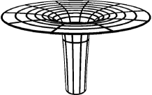
Under the hypothesis of this theorem (namely, electro-vacuum and axial symmetry) both the angular momentum and the electric charge are defined as conserved quasi-local integrals (we discuss this in detail in section 4). In particular, if the topology of the manifold is trivial (i.e. ), then these quantities are zero and hence theorem 3.1 reduces to the positive mass theorem. In order to have non-zero charge or angular momentum we need to allow non-trivial topologies, for example manifolds with two asymptotic ends as it is the case in theorem 3.1 (see figure 2). An important initial data set that satisfies the hypothesis of the theorem is provided by an slice in the non-extreme Kerr-Newman black hole in the standard Boyer-Lindquist coordinates.
This theorem has three main limitations: i) the initial data are assumed to be maximal. ii) there is no rigidity statement. iii) the data are assumed to have only two asymptotic ends. Let us discuss these points in more detail. The maximal condition plays a crucial role in the proof since it ensure a positive definite scalar curvature. A relevant open problem is how to remove this condition, we will discuss it in more detail in section 6.
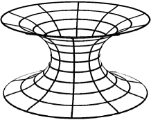
Extreme Kerr-Newman initial data, which reach the equality in (54), is not asymptotically flat in both ends. The data have a cylindrical end and an asymptotically flat end (see figure 3). Hence these data is excluded in the hypothesis of theorem 3.1. In order to include the equality case we need to enlarge the class of data. An example is given by the following theorem proved in [44] which includes the rigidity statement.
Theorem 3.2.
The precise definition of the Brill class of data can be seen in [44]. The main advantage of these kind of data is that they encompass both class of asymptotics: cylindrical and asymptotic flatness. We discuss this in section 5.1. The condition 2.5 (see [44] for details) mentioned in this theorem implies that the initial data have non trivial angular momentum only at one end, however multiple extra ends with zero angular momentum are allowed. This condition involves also other restrictions which are technical. In a very recent work [105] these technical conditions have been removed and also an interesting new approach to the variational problem is presented.
The inequality (54) (which in particular implies (55)) is expected to hold for manifolds with an arbitrary number of asymptotic ends, this generalization is probably to most important open problem regarding this kind of inequalities (we discuss this in detail in the final section 6). There exist, however, a very interesting partial result [33]. In order to describe it, we need to introduce the mass functional , this functional is defined in section 5. It plays a major role in all the proofs, as it is explained in section 3.3. This functional represents a lower bound for the mass. Moreover, the global minimum of this functional (under appropriate boundary conditions which preserve the angular momentum) is achieved by an harmonic map with prescribed singularities. As we will see in section 3.3 this is the main strategy in the proofs of all the previous theorem which are valid for two asymptotic ends. Remarkably enough in [33] the existence and uniqueness of this singular harmonic map has been proved also for manifolds with an arbitrary number of asymptotic ends. In this article the following theorem is proved.
Theorem 3.3.
Consider an axially symmetric, vacuum asymptotically flat and maximal initial data with asymptotic ends. Denote by , () the mass and angular momentum of the end . Take an arbitrary end (say ), then the mass at this end satisfies the inequality
| (56) |
where denotes the numerical value of the mass functional evaluated at the corresponding harmonic map.
This theorem reduces the proof of the inequality with multiples ends to compute the value of the mass functional on the corresponding harmonic map and verify the inequality
| (57) |
We further discuss this theorem in section 3.3.1.
Strong numerical evidences that inequality (57) holds for three asymptotic ends has been provided in [48]. The numerical methods used in that article are related with the harmonic map structure of the equations. We will describe them in section 5.2.
All the previous results assume complete manifolds without inner boundaries. The inclusion of inner boundary is important to prove the Penrose inequality with angular momentum (17). Boundary conditions in relation with the mass functional where studied in [61] in order to prove a version of Penrose inequality in axial symmetry. In [36] inner boundaries were also included and an interesting new lower bound for the mass is obtained which depends only on the inner boundary. Finally, we mention that in [80] numerical evidences for the validity of the Penrose inequality (17) has been presented.
3.2 Quasi-local inequalities
Quasi-local inequalities between area and charge has been proved in [59] for stable minimal surfaces on time symmetric initial data. The following theorem proved in [47] generalize this result for generic dynamical black holes.
Consider Einstein equations with cosmological constant
| (58) |
where is the electromagnetic energy-momentum tensor defined in terms of the electromagnetic field by (85). The electric charge of an arbitrary closed, oriented, two-surface embedded in the spacetime is defined by (86).
Theorem 3.4.
Given a closed marginally trapped surface satisfying spacetime stably outermost condition, in a spacetime which satisfies Einstein equations (58) with non-negative cosmological constant and such that the non-electromagnetic matter fields fulfill the dominant energy condition, the following inequality holds:
| (59) |
where and are the area and the charge of .
For the definition of marginally trapped surfaces (which is standard) and the stably condition see [2] [3] [79] [47] (see also [66] [98]). This theorem is a completely quasi-local result that applies to general dynamical black holes without any symmetry assumption. It is also important to emphasize that the matter is not assumed to be uncharged, namely it is allowed that (which is equivalent to ). The only condition imposed in the non-electromagnetic matter field stress-energy tensor is that it satisfies the dominant energy condition. In this theorem it is also possible to include the magnetic charge and Yang-Mills charges (see [47] and [77]).
In [107] an interesting generalization of theorem 3.4 is presented in which the stability requirement is removed at the expense of introducing the principal eigenvalue of the stability operator and also the cosmological constant (with arbitrary sign) is added.
At the end of section 2 we have observed that a variant of inequality (59) is expected to hold for ordinary macroscopic charged object (which are not necessarily black holes) at least if they are ‘round enough’. In fact there exists an interesting and highly non-trivial counter example to (59) for macroscopic objects. This counter example was constructed by W. Bonnor in [22] (see also the discussion in [47]) and it can be summarized as follows: for any given positive number , there exist static, isolated, non-singular bodies, satisfying the energy conditions, whose surface area satisfies . The body is a highly prolated spheroid of electrically counterpoised dust. From the physical point of view we are saying that for an ordinary charged object (in contrast to a black hole) we need to control another parameter (the ‘roundness’) in order to obtain an inequality between area and charge. Remarkably enough it is possible to encode this intuition in the geometrical concept of isoperimetric surface: we say that a surface is isoperimetric (or ‘round’) if among all surfaces that enclose the same volume as does, has the least area. Then, based on the results proved in [29] the following theorem was obtained in [47] for isoperimetric surfaces.
Theorem 3.5.
Consider an electro-vacuum, maximal initial data, with a non-negative cosmological constant. Assume that is a stable isoperimetric sphere. Then
| (60) |
where is the electric charge of .
Note that inequality (60) has a different coefficient as (59). We recall that the notion of stable isoperimetric surface is very similar to the case of a stable minimal surface: the differential operator is identical, the only difference is that the allowed test functions should integrate to zero on the surface, this is precisely the condition that the deformations preserve the volume (see [17]).
It is also possible to prove interesting variants of theorem 3.4 which are valid for generic surfaces (i.e. not necessarily trapped or minimal) but in order to obtain these results global assumptions on the initial data should be made (that is, in contrast to theorem 3.4, these are not a purely quasi-local results): the two surfaces are embedded on initial conditions that are complete, maximal and asymptotically flat. The non electromagnetic matter fields are assumed to be non charged and they should satisfy the dominant energy condition on the whole initial data (see Theorem 2.2 in [47]).
As in the case of the global inequality, quasi-local inequalities with angular momentum involve different techniques in comparison with the pure charged case. Their study star very recently.
The quasi-local inequality with angular momentum and charge (26) was first conjectured to hold in stationary spacetimes in [10]. In that article the extreme limit of this inequality was analyzed and also numerical evidences for the validity in the stationary case was presented (using the numerical method and code developed in [7]). In a series of articles [68] [69] the inequality (26) was proved for stationary black holes. See also the review article [6].
It is important to emphasize that the stationary non-vacuum case is highly non-trivial. The physical situation is, for example, a black hole surrounded by a ring of matter (which do not touch the black hole). To illustrate the complexity of this case we mention that the Komar mass (which is only defined in the stationary case) can be negative for these black holes (for the Kerr-Newman black hole is always positive), see [8] [9]. It is interesting to mention that for this class of stationary spacetimes there exists a remarkable relation of the form , where and denote the areas of event and Cauchy horizon. This result have been proved in the following series of articles [5] [67] [4].
In the dynamical regime, the inequality was conjectured to hold in [45] based on the heuristic argument mentioned in section 2. In that article also the main relevant techniques for its proof were introduced, namely the mass functional on the surface and its connections with the area (we discuss this in section 5.3). A global proof (but with technical restrictions) was obtained in [1] [55]. The first general and pure quasi-local result was proven in [50], where the relevant role of the stability condition for minimal surfaces was pointed out:
Theorem 3.6.
Consider an axisymmetric, vacuum and maximal initial data, with a non-negative cosmological constant. Assume that the initial data contain an orientable closed stable minimal axially symmetric surface . Then
| (61) |
where is the area and the angular momentum of . Moreover, if the equality in (61) holds then and the local geometry of the surface is an extreme Kerr throat sphere.
The extreme throat sphere geometry, with angular momentum , was defined in [45] (see also [1] and [50]). This surface capture the local geometry near the horizon of an extreme Kerr black hole and it is defined as follows. The sphere is embedded in an initial data with intrinsic metric given by
| (62) |
where is given by (201). Moreover, the sphere must be totally geodesic, the twist potential evaluated at the surface must be given by defined by (201) and the components of the second fundamental
| (63) |
must vanish at the surface. Here denotes the second fundamental form of the initial data, the unit normal vector to the surface and the axial Killing field. Note that the functions and , which characterize the intrinsic and extrinsic geometry of the surface respectively, depend only on the angular momentum parameter . The geometry of axially symmetric initial data set are described in detail in section 5.1. In particular, the twist potential is determined by the second fundamental form , using equation (175). The adapted coordinates system used in (62) is defined is section 4.1.
This theorem has two main restriction: the first one is the maximal condition. The second is vacuum. Remarkably enough, it is possible not only to avoid both restrictions but also to provide a pure spacetime proof (that is, no mention of a three-dimensional hypersurface) of this inequality, in which axisymmetry is only imposed on . This generalization is proved in [79]:
Theorem 3.7.
Given an axisymmetric closed marginally trapped surface satisfying the (axisymmetry-compatible) spacetime stably outermost condition, in a spacetime with non-negative cosmological constant and fulfilling the dominant energy condition, it holds the inequality
| (64) |
where and are the area and (Komar) angular momentum of . If equality holds, then is a section of a non-expanding horizon with the geometry of extreme Kerr throat sphere.
The concept of non-expanding horizon is explained in [79], it essentially means that the shear vanished at the surface.
It is important to note that the angular momentum that appears in (64) is the gravitational one (i.e. the Komar integral). The matter fields have also angular momentum and it can be transferred to the black hole, however the inequality (64) remains true even in that case. In fact this inequality is non-trivial for the Kerr-Newman black hole, we discuss this in detail in section 4.
In [99] it has been pointed out that there exists a connexion between the global inequalities described in section 3.1 and the quasi-local inequalities. This is obtained by linking the relevant mass functional and (we discuss these mass functional in section 3.3).
3.3 Main ideas
In this section we present the main ideas behind the proofs of the global inequality (54) and the quasi-local inequality (64). This section should be consider as a guide in which the technicalities are avoided. In section 4 and 5 we discuss in details the main relevant properties of the angular momentum and mass in axial symmetry which constitute the essential part of the proofs.
3.3.1 Global inequalities
The starting point in the proof of the inequality (54) (we consider the case for simplicity) is the formula for the total mass given by Eq. (184). This formula represents the total mass as a positive definite integral over a maximal (here is where the maximal condition plays a crucial role) initial surface. This integral representation is a generalization of the Brill mass formula discovered in [26] (in section 5 we further discuss this formula and provide the relevant references). The formula holds in a particular coordinate system which is called isothermal (see lemma 5.1).
The integrand in Eq. (184) has two kind of terms: dynamical and stationary. The dynamical terms vanished for an stationary solution like Kerr. The stationary part lead to the relevant mass functional defined by (185). This functional provides an obvious lower bound to the total mass, namely
| (65) |
The mass functional depends on two functions and . The function is essentially the norm of the axial Killing vector (see equation (179)). The function is the twist potential of the Killing vector (see section 4). These two functions can be freely prescribed on the initial data. This is an important and far from obvious property since the constraint equations (162)–(163) should be satisfied. This fact allows to formulate a variational principle for the functional . The other important ingredient for this variational principle is the behavior of the angular momentum. The angular momentum is prescribed by the value of at the axis (see section 4). Then, if the variations of vanishes at the axis the angular momentum will be preserved. With this two ingredients, it is hence possible to reduce the proof of the inequality (54) to a pure variational problem for the functional .
The second step of the proof is to solve this variational problem. This is the most difficult part and also the most interesting since it reveals the geometric properties of the mass functional . Let us discuss the general strategy of the proof.
Let be the corresponding functions obtained from the extreme Kerr initial data with angular momentum , then we have that
| (66) |
The heuristic discussed in section 2 and Eq. (67) suggest that the following inequality holds
| (67) |
for all such that has the same value at the axis as the function . Moreover, the equality in (67) is reached if and only if and . This is precisely the variational problem. Note the variational problem is formulated purely in terms of the functional , without any reference to the constraint equations (162)–(163).
The first evidence that this variational problem will have the expected solution is that the Euler-Lagrange equations of the functional are equivalent to the stationary axially symmetric Einstein equations, in particular extreme Kerr satisfies these equation [41]. The second evidence (which is harder to prove) is that the second variation of is positive definite evaluated at extreme Kerr [40]. To prove this positivity property it is crucial to make contact with the harmonic map theory (in this case, trough the Carter identity). With these ingredients it is possibly to show that extreme Kerr is a local minimum of the mass and hence the inequality (67) is proved in an appropriate defined neighborhood of extreme Kerr. This local proof was done in [40].
To have a global proof of (67) (i.e. without any smallness assumption) more subtle properties of the mass functional are required. A crucial step is to realize that the mass functional is essentially the renormalized energy of an harmonic map into the hyperbolic plane [44] (we discuss this in section 5.2). This kind of harmonic maps have been extensive studied in the literature. The problem here is that the map is singular at the axis and hence the standard techniques do not apply directly. To use the harmonic map theory we need to handle these singularities and this is the main technical difficulty. In [44] the proof of this variational result was done using estimates, inspired in the work of G. Weinstein [111] [112] [113] [114] [116] [115] (see also [86])), which rely on particular properties of this functional (inversion symmetry). In subsequent works [31], [33], [35], [38] the proof was simplified and improved using general results on harmonic maps (more precisely the existence result [71]). In these proofs the connection with the harmonic maps theory is more transparent and the problem of the singularities is clearly isolated.
Finally let us mention the following important point regarding initial data with multiples ends. The multiples ends appears in the variational problem (67) as singular points of the functions . Remarkably, even in that case it is possible to solve completely the variational problem. This is precisely the content of theorem 3.3 (proved in [33]). The only missing piece in order to prove the inequality (54) in that case is the following. Theorem 3.3 ensure the existence of a global minimum but the value of at the global minimum is unknown. In the case of two asymptotic ends we known that extreme Kerr is the global minimum and hence we can explicitly compute the value (66).
3.3.2 Quasi-local inequalities
The global inequality (54) applies to a complete three dimensional manifold. In contrast the quasi-local inequality (64) apply to a closed two-surface. In principle it is a priori not clear at all that there is a relation between these two kind of inequalities. The two physical heuristic argument presented in section 2 in support for them are very different. In particular, it is far from obvious that the mass functional can play a role for the quasi-local inequalities. Remarkably enough, it turns out that a suitable adapted mass functional over a two-surface play a very similar role as . The motivation for the definition of given by (204) is discussed in section 5.3. The new mass functional and its connection with the area represent the kernel of the proof of (64). Let us discuss this.
On the extreme Kerr initial data there exist an important canonical two-surface, namely the intersection of the Cauchy surface with the horizon. On a surface given by in the Boyer-Lindquist coordinates this two-surface is located at infinity on the cylindrical end (see figure 3). Let call the value of the functions (defined in the previous section 3.3.1) on this two-surface. The functions will play for a similar role as the functions for . Namely, first they satisfy the Euler-Lagrange equations of . Second, the second variation of is positive definite evaluated at (see [45]). There is also a connection with the harmonic maps energy (we discuss this in section 5.3). Using similar kind of arguments as described in section 3.3.1 it is possible to prove the following inequality
| (68) |
for all functions such that has the same values at the poles of the two-surface as . With equality if and only if we have and . A local version of this inequality was first proved in [45]. The global version (68) was proved in [1]. The rigidity statement was proved in [50]. We emphasize that the inequality (68) (in complete analogy to the inequality (67)) is a property of the functional , the geometry of the two-surface does not intervene at all.
The inequality (68) is interesting but, in the light of the discussion presented in 3.3.1, it is somehow expected. What is crucial and completely unexpected is the relation between and the area of the surface . This relation was founded locally in [45] and globally in [1]. By local in this context we mean that the relation holds for surfaces in an appropriated defined neighborhood of an extreme Kerr throat geometry. On the other hand, global means that the relation holds for general surfaces. In [50] the important connection with the stability condition was proved for minimal surfaces and in [79] for marginally trapped surfaces. The final inequality essentially reads as follows. For a two-surface such that: (i) it is minimal [50] (or marginally trapped [79]) and (ii) it is stable, then the following inequality holds
| (69) |
The minimal and marginally trapped conditions are requirements on the extrinsic curvature of (namely, on the trace of the second fundamental form). The stability condition is a requirement on derivatives of the second fundamental form. In the spacetime version presented in [79]) the inequality (69) is a consequence of a flux inequality (see Lemma 1 in that reference) where the geometric and physical meaning of each term is apparent.
4 Angular momentum in axial symmetry
Axial symmetry plays a major role in the inequalities that include angular momentum presented in the previous sections for two main reasons. For the global inequality (54) is the conservation of angular momentum implied by axial symmetry which is relevant. For the quasi-local inequality (61), is the very definition of quasi-local angular momentum (only possible in axial symmetry) which is important. These two properties are closed related for vacuum spacetimes, since the Komar integral provides both the conservation law and the definition of quasi-local angular momentum. For non-vacuum spacetimes in axial symmetry the Komar integral still provides a meaningful expression for the gravitational angular momentum but it is no longer conserved. Nevertheless, as we already mentioned in section 2, in the electro-vacuum case the sum of the gravitational and electromagnetic angular is conserved, and hence in that case is possible to prove the global inequality (54). In the general non-vacuum case in axial symmetry (that is, with general matter sources which are not electromagnetic) no simple and universal relation between mass and angular momentum is expected. For example in [58] neutron starts models in axial symmetry have been numerically constructed such that they violate inequality (54). Nevertheless, remarkably, the quasi-local inequality (61) for black holes is still valid in the general non-vacuum axially symmetric case.
In this section we summarize relevant results concerning angular momentum in axial symmetry. Although these results are not new they are not easy to find in the literature, notably, the conservation of angular momentum in the electro-vacuum case and the relation between Komar integrals and potentials in the presence of matter fields. The conservation of angular momentum in the electro-vacuum, together with the relevant Komar integral for the electromagnetic angular momentum, were discovered in [106], in a much general setting. We present a simpler derivation of this result in the language of differential forms.
Let us begin with some general remarks about conserved quantities in General Relativity (see also the review article [78] for a related discussion and [108] for the general problem of how to define quasi-local angular momentum without symmetries).
Let be a four dimensional manifold with metric (with signature ) and Levi-Civita connection . On this curved background, let us consider an arbitrary energy-momentum tensor which satisfies the conservation equation
| (70) |
It is well known that if the spacetime admit a Killing vector field
| (71) |
then the vector
| (72) |
is divergence free
| (73) |
This equation provides an integral conservation law via Gauss theorem. For some of the computations in this section it is convenient to use differential forms instead of tensors. We will denote them with boldface. Let be the 1-form defined by (72). Equation (73) is equivalent to
| (74) |
where is the exterior derivative and the dual of a form is defined with respect to the volume element of the metric by the standard formula
| (75) |
Let denotes a four-dimensional, orientable, region in and let be its three-dimensional boundary. Then using (74) and the Stokes theorem we obtain
| (76) |
Note that in this equation the region is arbitrary and the boundary can have many disconnected components.
Consider a spacelike three-surface . The conserved quantity corresponding to the Killing vector is defined with respect to by
| (77) |
The interpretation of equation (76) in relation to the quantity is the following. Let to be a timelike cylinder, such that its boundary is formed by the bottom and the top spacelike surfaces and and the timelike piece . Then we have (taking the corresponding orientation)
| (78) |
The integral over the timelike surface is the flux of . Equation (78) is interpreted as the conservation law of the quantity . The region can also be chosen to have a null boundary , equation (78) remains identical and the interpretation is similar.
If the Killing vector is also a symmetry of the tensor (we have not assumed that so far), namely
| (79) |
where denote Lie derivatives, then the following vector is also divergence free
| (80) |
where is the trace of . In fact there is a whole family of divergence free tensors since is divergence free. Hence the previous discussion applies to this vector as well.
Note that the conserved quantities are naturally defined as integrals over spacelike three-surfaces. In flat spacetime it is possible to convert these integrals into a boundary integral over two-surfaces. This gives the quasi-local representation of conserved quantities (see the discussion in the introduction of [108]). In a curved background this is in general not possible. However, as we will see, this possible for the particular case of the electromagnetic field.
Before analyzing the angular momentum it is important to study the electric charge. The electric charge is of course relevant in our discussion since it appears in the inequalities discussed in the previous sections. But more important, even if we want to analyze these inequalities in pure vacuum, the electric charge represent the simpler ‘conserved charge’ on a curved spacetime. Its definition and properties serve as model for all the other conserved quantities, like the angular momentum.
The Maxwell equations on are given by
| (81) | ||||
| (82) |
In terms of forms, they are written as
| (83) | ||||
| (84) |
The energy-momentum tensor of the electromagnetic field is given by
| (85) |
Let be a closed orientable two-surface embedded in (in the following, all two-surfaces will be assumed to be closed and orientable). The electric charge of is defined by
| (86) |
Let be a three-surface with boundary , then using Stokes theorem and Maxwell equation (83) we obtain
| (87) |
This equation is interpreted as follows. From equation (83) we deduce the conservation law for the current analog to (74), namely
| (88) |
And hence taking the same region and using Stokes theorem we obtain the analog expression as (78) for the current
| (89) |
Using (87) we finally obtain
| (90) |
This is the conservation law for the electric charge. Note that in the left hand side of (90) we have integrals over two-surfaces, in contrast with (78) where integrals over three-surfaces appear. This is because we have an extra equation (i.e. Maxwell equation (83)) that allow us to write the integral (87) in the form (86).
When the charge has the same value, namely
| (91) |
and we say that the charge is strictly conserved.
We turn now to angular momentum for axially symmetric spacetimes. We begin with the definition of axial symmetry.
Definition 4.1.
The spacetime is said to be axially symmetric if its group of isometries has a subgroup isomorphic to .
We will denote by the Killing field generator of the axial symmetry. The orbits of are either points or circles. The set of point orbits is called the axis of symmetry. Assuming that is a surface, it can be proved that is spacelike in a neighborhood of (see [89]). We will further assume that the Killing vector is always spacelike outside . Note that if this condition is not satisfied then the spacetime will have closed causal curved, in particular it can not be globally hyperbolic.
The form will be denoted by , and the square of its norm by , namely
| (92) |
We have used the notation to denote the Killing vector field and to denote the square of its norm to be consistent with the literature. However, in this section, to avoid confusions between and its square norm , we will denote the vector field by in equations involving differential forms in the index free notation.
Consider now Einstein equations on an axially symmetric spacetime
| (93) |
Note that the Killing equation (71) implies that satisfies (79).
The Komar integral (it is also appropriate to call it the Komar charge) of the Killing field is defined over a two-dimensional surface as follows
| (94) |
Hence, as we discussed above, via Stokes theorem we obtain
| (95) |
where is a three-dimensional surface with boundary . It is a classical result [82] (see also [110]) that the integrand in (95) can be computed in terms of the Ricci tensor
| (96) |
In terms of forms this equation is written as
| (97) |
where we have defined the 1-form by
| (98) |
Using Einstein equations (93) the form can be written in terms of the energy momentum tensor
| (99) |
Note that this expression is identical to (80). Then, repeating the same argument, we obtain the conservation law for angular momentum in axial symmetry which is the exact analog to the charge conservation (90)
| (100) |
The right hand side of this equation represent the change in the angular momentum of the gravitational field which is produced by the left hand side, namely the angular momentum of the matter fields. Note that the angular momentum of the matter fields are written as integrals over three-dimensional surfaces. In particular in vacuum we have the strict conservation of angular momentum
| (101) |
We consider now the case where the energy-momentum tensor in Einstein equations (93) is given purely by the electromagnetic field (85). For simplicity we consider the case with no currents , which is the relevant one since only in that case we get conserved quantities. In that case we have that (85) satisfies the equation (70) and the source-free Maxwell equations are given by
| (102) | ||||
| (103) |
We also assume that the Maxwell fields are axially symmetric, namely
| (104) |
Consider the 1-forms defined by
| (105) |
where we have used the standard notation to denote contractions of forms with vector fields. Using the general expression for the action of the Lie derivative on forms
| (106) |
Maxwell equations (102)–(103) and the condition (104) we obtain
| (107) |
It follows that there exist locally functions and such that
| (108) |
The form defined by (99) has the following expression for the electromagnetic field
| (109) |
We have that (see [116])
| (110) |
Using (108) we obtain
| (111) |
and hence there exist locally a 1-form such that
| (112) |
where is given by
| (113) |
Note that
| (114) |
From equation (110) we deduce
| (115) |
We use the following identity valid for arbitrary 1-forms
| (116) |
Using (112) we finally obtain our main formula
| (117) |
where we have defined
| (118) |
It is important to note that
| (119) |
Using equation (117), we integrate over a three-surface tangential to , with boundary . Using that is tangential to it follows that the restriction of the 3-form to is zero. For the second term in (117) we use equations (114) and (119) to obtain the same conclusion. Hence, we have
| (120) |
where in the last equality we have used Stokes theorem.
We summarize the previous calculation in the following lemma, which is a re-writing of the result that have been obtained in [106].
Lemma 4.2.
Consider an axially symmetric spacetime for which the Einstein-Maxwell equations (93), (85), (102), (103) are satisfied. Let be an orientable three-surface, tangent to the axial Killing field , with boundary (possible disconnected) . Then we have
| (121) |
where is the Komar integral given by (94), is defined in terms of the electromagnetic field by (113) and is given by (118).
We can define a ‘total angular momentum’ which is conserved in electro-vacuum, namely
| (122) |
We note that since the surface is tangent to and all the fields are axially symmetric, then the surface integrals are in fact line integrals on the quotient manifold .
Formula (122) was studied in [13][12] for rotating isolated horizons. This formula has been also recently studied at null infinity in connection with the center of mass and general definition of angular momentum for asymptotically flat (at null infinity) spacetimes, see [83].
A very important example where lemma 4.2 applies is the Kerr-Newman black hole. Consider the Kerr-Newman black hole with parameters . The total angular momentum is given by . This is equal to the Komar integral evaluated at infinity, since the electromagnetic field decay and does not contribute at infinity. However at the horizon the Komar angular momentum is not . The angular momentum at the horizon has the decomposition (122).
For the Kerr-Newman black hole the Komar angular momentum at the horizon is given by (see, for example, [97] page 222).
| (123) |
where is the horizon radius
| (124) |
The area of the horizon is given by
| (125) |
Equation (125) is of course identical to equation (8). As we already mentioned, it is well known that the area satisfy the inequality
| (126) |
Which in particular implies
| (127) |
But this inequality relates the total angular momentum . It is a priori not obvious if the following inequality holds
| (128) |
where is given by (123), namely the Komar integral at the horizon. Note that this is precisely the inequality proved in theorem 3.6 and that the Kerr-Newman black hole satisfies all the hypothesis of that theorem.
Let us check explicitly that indeed (128) is satisfied. The expression (123) is remarkably complicated, to better analyze it let us rewrite it in the following form. Using (125) we have
| (129) |
where
| (130) |
Instead of using it is convenient to use as free parameter. In terms of the function is written us
| (131) |
where
| (132) |
We take as free parameters . Note that and hence we have
| (133) |
Fix . It can be explicitly check that function is non-positive and have a unique global minimum at where . Hence it follows that
| (134) |
4.1 Potentials
The potentials for the axial Killing vector plays an important role in the mass functional described in section 5.
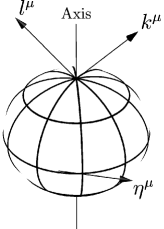
It is instructive to analyze first the electric charge and its potential in axial symmetry. Assume first that the Maxwell equations are source free. Then we have found the potentials and defined by equation (108). In particular, the potential determine the electric charge over an axially symmetric two-surface . In order to see that it is convenient to consider a tetrad and coordinate system adapted to an axially symmetric two-surface defined as follows (see figure 4). For simplicity we will assume that has the topology of a two-sphere. Let us consider null vectors and spanning the normal plane to and normalized as , leaving a (boost) rescaling freedom , . By assumption is tangent to , it has on the surface closed integral curves and vanishes exactly at two points which are the intersection of the axis with . We normalize vector so that its integral curves have an affine length of . Let us chose a coordinate on such that . The other vector of the tetrad which is tangent to and orthogonal to will be denoted by and assume that it has unit norm. We define the coordinate such that is proportional to and such that are the poles of .
The induced metric and the volume element on (written as spacetime projectors) are given by and respectively. The area measure on is denoted by . Since the surface is axially symmetric we have .
Using this tetrad, the charge over an axially symmetric surface is written as follows
| (135) |
where is defined by (105). In the source free case we can use the potential defined by (108) to obtain
| (136) |
That is, the charge is given by the difference of the value of the potential at the poles of the surface .
We have seen that the potential is only defined in the source-free case as scalar function in the spacetime. However, on the surface it is always possible to define a potential by the equation
| (137) |
on the surface, since this equation involves only a derivative with respect to . The potential is only defined on the surface. By definition, in the source-free case where the potential also exists, the two functions are equal up to a constants on the surface. This constant is irrelevant since it does not affect the charge.
Consider now the potential for the angular momentum. The twist vector of is defined by
| (138) |
It is a well known result that the vacuum equations imply that
| (139) |
where is the 1-form defined by (138). Hence there exist a potential such that
| (140) |
The function is the twist potential of the Killing vector , it contains all the information of the angular momentum as we will see. In the non-vacuum case, the twist potential is not defined. In the following we will not assume vacuum.
In terms of the adapted tetrad we have that the Komar expression is given by
| (141) |
We the relation
| (142) |
to write the Komar integral in the following form
| (143) |
It is clear that the vector defined by
| (144) |
is orthogonal to and it has unit norm and hence is the other member of the tetrad. Then we have
| (145) |
We emphasize that this expression is valid only for axially symmetric surfaces.
If we assume vacuum, then we can use the twist potential defined by (140) to obtain
| (146) |
Equations (145) and (146) are the analog to equations (135) and (136) for the charge.
We consider now the non-vacuum case. We define the following vector (a part of the extrinsic curvature of with the role of a connection on its normal cotangent bundle, see e.g. the discussion in [63] [23])
| (147) |
Since is axially symmetric, the tetrad can be chosen such that
| (148) |
In particular this implies that
| (149) |
Using this equation we obtain that
| (150) |
From this equation we get the following equivalent expression for the Komar angular momentum (see, for example, [78])
| (151) |
Remarkably, as we will see in the following, the vector determines even in the non-vacuum case a potential on the surface (we will denote it by ) which coincide with the twist potential defined above in the vacuum case. We emphasize that the potential will be only defined on the two-surface , in contrast to the twist potential which (in the vacuum case) is defined by equations (139) and (140) on a region of the spacetime.
By construction, the vector is tangent to the surface . Since we have assumed that has the topology, there exists functions and such that the vector has the following decomposition on in terms of a divergence-free and an exact form
| (152) |
The functions and are fixed up to a constant. In equation (152) we have used the capital indices (which run from to ) to emphasizes that this is an intrinsic equation on the two-surface .
By assumption both and the intrinsic metric on are axially symmetric, then it follows that the functions and are also axially symmetric (i.e. they depend only on ). In particular it follows that
| (153) |
where is the vector tangent to previously defined. Since the norm is also an axially symmetric function, equation (153) implies that
| (154) |
Equation (154) ensures the integrability conditions for the existence of a function such that
| (155) |
Note that equation (155) is valid only in axial symmetry. Collecting these results we obtain the decomposition
| (156) |
In particular, using (153), we obtain
| (157) |
We write equation (157) with spacetime indices and we use the following representation for the tetrad vector
| (158) |
to finally obtain
| (159) |
Using equation (151) an integrating we finally get
| (160) |
The relevance of this construction is that the function , which is only defined at the surface , plays the role of a potential that can be defined in the non-vacuum case [79]. To see the relation between and , note that we have
| (161) |
This equation is valid always (i.e. non-vacuum) and it gives the function in terms of the twist vector . In the non-vacuum case the twist potential is not defined but the function is always well defined. In fact, we can take (161) as definition of , since the right hand side is only a derivative with respect to . On the other hand, in the vacuum case equation (161) implies that and differs by a constant which is irrelevant since it does not contribute to the angular momentum.
5 Mass in axial symmetry
The main goal of this section is to present the mass formula for axially symmetric data (184) and the mass functional for two-surfaces (204). We also discuss their geometrical properties in connection with harmonic maps.
5.1 Axially symmetric initial data
The global geometrical inequality (54) is studied on axially symmetric, asymptotically flat initial data set. In order to present the mass formula, we first review the basic definitions and properties of this kind of initial data. For simplicity we concentrate only in the pure vacuum case (see [35] [38] for the electro-vacuum case).
An initial data set for the Einstein vacuum equations is given by a triplet where is a connected three-dimensional manifold, a Riemannian metric, and a symmetric tensor field on . The fields are assumed to satisfy the vacuum constraint equations
| (162) | |||
| (163) |
where and are the Levi-Civita connection and the scalar curvature associated with , and . In these equations the indices are moved with the metric and its inverse .
The initial data is called maximal if
| (164) |
This condition is crucial because it implies via the Hamiltonian constrain (163) that the scalar curvature is non-negative. In fact on the right hand side of equation (163) it is possible to add a non-negative matter density and all the arguments behind the proof of theorem 3.1 will also apply since they rely on lower bounds for .
The manifold is called Euclidean at infinity, if there exists a compact subset of such that is the disjoint union of a finite number of open sets , and each is diffeomorphic to the exterior of a ball in . Each open set is called an end of . Consider one end and the canonical coordinates in which contains the exterior of the ball to which is diffeomorphic to. Set . An initial data set is called asymptotically flat if is Euclidean at infinity, the metric tends to the euclidean metric and tends to zero as in an appropriate way. These fall off conditions (see [18] [30] for the optimal fall off rates) imply the existence of the total mass (or ADM mass [11]) defined at each end by
| (165) |
where denotes partial derivatives with respect to , is the euclidean sphere in , is its exterior unit normal and is the surface element with respect to the euclidean metric.
The angular momentum is also defined as a surface integral at infinity (supplementary fall off conditions must be imposed, see, for example, the review articles [108], [78] and reference therein). Let be an infinitesimal generator for rotations with respect to the flat metric associated with the end , then the angular momentum in the direction of is given by
| (166) |
The above discussion applies to general asymptotically flat initial data. We have seen that at any end the total mass and the total angular momentum are well defined quantities. We consider now axially symmetric initial data. In analog way as the spacetime definition 4.1, we say that the Riemannian manifold is axially symmetric if its group of isometries has a subgroup isomorphic to . We will denote by the Killing field generator of the axial symmetry and by the axis. The initial data set is called axially symmetric if in addition is also a symmetry of , namely
| (167) |
On an axially symmetric spacetime there exist axially symmetric initial condition, conversely axially symmetric initial data evolve into an axially symmetric spacetime. However, on an axially symmetric spacetime it is also possible to take initial conditions which are not axially symmetric in the sense defined above. These conditions will of course also evolve into an axially symmetric spacetime, but the Killing vector is ‘hidden’ on them (these kind of initial data were studied in [20]). We will not consider this kind of data here since on an axially symmetric spacetime it is always possible to chose initial conditions which are explicitly axially symmetric in the sense defined above.
For axially symmetric data we have the Komar integral discussed in section 4. This integral can be calculated in terms on the initial data if we chose . There exist a very simple relation expression for the Komar integral on an initial data, namely
| (168) |
The equivalence between (168) and the original definition (94) can be seen as follows. Consider the tetrad adapted to defined in section 4.1. Assume that . By assumption, the axial Killing vector is tangent to the three-dimensional surface . Denote by the timelike unit normal to the three-surface , and let be the spacelike unit normal to the two-surface which lies on . These vectors can be written in term of and as follows
| (169) |
Using these expression, we can write the integrand in (94) as
| (170) |
The second fundamental form can be written (as spacetime tensor) in terms of the unit normal as
| (171) |
Using that and that is tangent to , from (171) we obtain
| (172) |
Comparing expression (168) with (166) we see that if we chose in (166) the vector (that it, the generator of axial rotations) then these to expression are equivalent since for an sphere at infinity.
It is possible to calculate the potential for the spacetime Killing field defined in section 4 in terms of as follows. Define the vector by
| (173) |
where is the volume element with respect to the metric . Then, as a consequence of equations (162) and (167) we have that
| (174) |
Then the potential is defined by
| (175) |
It can be checked that this is the same potential as defined in the previous section (see [42]) evaluated on the initial surface. The importance of the expression (175) is that allow to calculate in terms of the initial conditions.
The functions and have the information of the stationary part of the initial conditions. The dynamical part is characterized by the functions and defined by
| (176) |
The notation comes from the fact that they are related with the time derivative of this functions, namely if is the timelike normal of the initial data, we have (see [42])
| (177) |
The whole initial data can be constructed in terms of . These functions are the initial data for the wave map equations that characterize the evolution in axial symmetry. This is clearly seen in the quotient representation (see [49]). For our present purpose the relevant part of the initial conditions is contained in .
So far we have discussed local implications of axial symmetry. Suppose that is simply connected and asymptotically flat (with, possible, multiple ends). It can be proved (see [31]) that in such case the analysis essentially reduces to consider manifold of the form where are points in . These points represent the extra asymptotic ends of . Moreover, in [31] it has been proved that on there exists the following global coordinate systems which will be essential in what follows.
Lemma 5.1 (Isothermal coordinates).
Consider an axially symmetric, asymptotically flat (with possible multiple ends) Riemannian manifold , where is assumed to be simply connected. Then, there exist a global coordinate system system such the metric has the following form
| (178) |
where the functions do not depend on . In these coordinates, the axial Killing vector is given by and the square of its norm is given by
| (179) |
Using this coordinates system, the end points are located at the axis of . Define the intervals , , to be the open sets in the axis between and , we also define and as and respectively (see figure 5). The manifold is Euclidean at infinity with ends. In effect, for each take a small open ball of radius , centered at , where is small enough such that does not contain any other with . Let be a closed ball, with large radius , such that contains all points in its interior. The compact set is given by and the open sets are given by , for , and is given by . Our choice of coordinate makes an artificial distinction between the end (which represent ) and the other ones. This is convenient for our purpose because we want to work always at one fixed end. We emphasize that the isothermal coordinates (and hence the corresponding spherical radius ) are globally defined on . In what follows we will always use these coordinates.
The smoothness of the initial data on the axis implies that the potential is constant on each interval . These constants are directly related with the angular momentum of the end points . In effect, the angular momentum of an end is defined to be the Komar integral with respect to a surface that encloses only that point. Using the formula (146) we obtain
| (180) |
Let a surface that enclose all the end points , then the total angular momentum of the end is given by
| (181) |
which is equivalent to
| (182) |

The mass (165) is defined as a boundary integral at infinity. For axially symmetric initial data there is an equivalent representation of the mass as a positive definite integral over the three-dimensional slice. This formula was discovered by Brill [26] and allow him to prove the first version of the positive mass for pure vacuum axially symmetric gravitational waves. This formula was generalized to include metrics with non hypersurface orthogonal Killing vectors (i.e. with non-zero and in the representation (178)) in [61] and for non-trivial topologies in [41]. In particular, this includes the topology of the Kerr initial data. See also [42] and [49] for related discussion on this mass formula.
Take isothermal coordinates and assume that the initial data are maximal (i.e. condition (164) holds). Then the total mass (165) is given by the following positive definite integral
| (183) |
where and is the flat volume element in , namely . Since the functions are axially symmetric the integration in is trivial, we keep however this notation because it will be important in section 5.2.
The remarkable fact of the integral (183) is that it applies also to the case of multiples ends, the integral is taking over all the extra ends since it cover the whole .
The integrand in (183) can be further decomposed as follows (see [49] for details)
| (184) |
Where the term is essentially the square of the second fundamental form of the two-surface that is obtained by the quotient of the manifold by the symmetry (this two-surface is a half plane minus the end points ). The important point in this representation is that it clearly separates the dynamical and the stationary terms in the mass formula. In fact, this formula can be seen as the geometrical conserved energy of the wave map that appear in the evolution equations (see [49]).
The first three terms in the integrand of (184) correspond to the dynamical part for the mass. They vanished for stationary solutions. The last two terms correspond to the stationary part. They give the total mass for Kerr. Explicitly the stationary part is given by
| (185) |
An hence we obtain the important bound
| (186) |
We have presented the mass formula but we have not discussed the asymptotic conditions that ensures that this integral is well defined. We discuss them now trying to focus only in the essential aspects, for the technical details we refer to [44] and [31]. All the important features can be seen already in the term in (185). We will concentrate in this term only in what follows.
It is instructive to see how the function behaves for the Kerr black hole initial data with mass . These initial data have two asymptotic ends, namely we have only one extra end point . In the limit (that is, the end ) we have
| (187) |
At the end we have
| (188) |
for the non-extreme case, and
| (189) |
for the extreme case. We see that the fall off behavior at the end is different for the non-extreme and extreme case, this reflect of course the difference between an asymptotically flat end and a cylindrical end (see figures 2 and 3 respectively).
To include this kind of fall off behavior let us consider the following conditions. In the limit we impose
| (190) |
At the end point we impose
| (191) |
Despite the formal similarity of (191) and (190) they are of a very different nature. Conditions (190) are essentially the standard asymptotic flat conditions on the metric, they include in particular the behavior (187) of the Kerr initial data. On the other hand, conditions (191) on the extra ends are much more general than asymptotic flatness. Note that asymptotic flatness at the ends in these coordinates essentially implies a behavior like (190). But conditions (188) includes also (189) (in fact also any logarithmic behavior with any coefficient).
The motivation for the fall off conditions (191) and (190) is that they ensures that the integral of is finite both at infinity and at the end points . And the advantage of condition (191) is that it encompasses both kind of behavior: asymptotically flat and cylindrical. This is the main motivation of the Brill data definition that appears in theorem 3.2 (see [44] for details).
5.2 Harmonic maps
The crucial property of the mass functional defined in (185) is its relation to the energy of harmonic maps from to the hyperbolic plane : they differ by a boundary term. To see this relation consider first the mass functional defined on a bounded region such that does not intersect the axis (given by )
| (192) |
We consider this integral for general functions and which are not necessarily axially symmetric. The function is harmonic outside the axis, that is
| (193) |
where is the flat Laplacian in . Using equation (193) we obtain the following identity
| (194) |
where the derivative is taken in the normal direction to the boundary and is given by
| (195) |
Recall that is defined by (179).
The functional defines an energy for maps where denotes the hyperbolic plane , equipped with the negative constant curvature metric
| (196) |
The Euler-Lagrange equations for the energy are given by
| (197) | ||||
| (198) |
The solutions of (197)–(198), i.e, the critical points of , are called harmonic maps from . Since and differ only by a boundary term, they have the same Euler-Lagrange equations.
Harmonic maps have been intensively studied, in particular the Dirichlet problem for target manifolds with negative curvature has been solved [64] [101] [100], and [71]. The last article is particularly relevant here. However, these results do not directly apply in our case because the equations are singular at the axis. One of the main technical complications in the proof of theorem 3.1 and 3.2 is precisely how to handle the singular behavior at the axis.
We present in what follows the main strategy in the proof of the inequality (67) (we follow the approach presented in [33] and [38]). The core of the proof is the use of a theorem due to Hildebrandt, Kaul and Widman [71] for harmonic maps. In that work it is shown that if the domain for the map is compact, connected, with nonvoid boundary and the target manifold has negative sectional curvature, then minimizers of the harmonic energy with Dirichlet boundary conditions exist, are smooth, and satisfy the associated Euler-Lagrange equations. That is, harmonic maps are minimizers of the harmonic energy for given Dirichlet boundary conditions. Also, solutions of the Dirichlet boundary value problem are unique when the target manifold has negative sectional curvature. Therefore, we want to use the relation between and the harmonic energy in order to prove that minimizers of are also minimizers of . There are two main difficulties in doing this. First, the harmonic energy is not defined for the functions that we are considering if the domain of integration includes the axis. Second, we are not dealing with a Dirichlet problem. To overcome these difficulties an appropriate compact domain is chosen which do not contain the singularities. Then a partition function is used to interpolate between extreme Kerr initial data outside this domain and general data inside, constructing also an auxiliary intermediate region. This solves the two difficulties in the sense that now the Dirichlet problem on compact region can be considered, and the harmonic energy is well defined for this domain of integration. This allows us to show that the mass functional for Kerr data is less than or equal to the mass functional for the auxiliary interpolating data. The final step is to show that as we increase the compact domain to cover all the auxiliary data converges to the mass functional for the original general data. This is the subtle and technical part of the proof.
Finally, we mention that it is possible to construct a heat flow for equations (197)–(198). Note that the first existence result for harmonic maps used a heat flow [53]. In our present setting, an appropriate heat flow that incorporates the singular boundary conditions is constructed as follows. Consider functions which depend on an extra parameter . Then, we define the following flow
| (199) | ||||
| (200) |
where a dot denotes partial derivative with respect to . Equations (199)–(200) represent the gradient flow of the energy (185). The important property of the flow is that the energy is monotonic under appropriate boundary conditions. This flow have been used in [48] as an efficient method for computing numerically both the solution and the value of the energy at a stationary solution.
5.3 Two surfaces and the mass functional
In this section we want to define a mass functional over a two-surface . This functional plays a major role in the proofs of the quasi-local inequalities. Let us motivate first the definition.
Consider the mass functional (185) defined over . Assume that on we have a foliation of two-surfaces. For example, take spherical coordinates and the two-surfaces . We can split the integral (185) into an integral over the two surface and a radial integral. However, the integral over the two-surface alone will not have any intrinsic meaning since, of course, its integrand depends on . To obtain an intrinsic expression we need somehow to avoid the dependence taking some kind of limit. For extreme Kerr initial data this limit is provided naturally on the cylindrical end. The functions and have a well defined and non-trivial limit there (in contrast with the asymptotic flat end where they tend to zero). Also, all the radial derivatives go to zero at the cylindrical end. This surface define an extreme Kerr throat surface (see the discussion in [46] and [45] for more details) and it characterized by only one parameter: the angular momentum . Explicitly the functions in that limit are given by
| (201) |
And the area of this two-surface is given by
| (202) |
Consider the following functional over a two-sphere
| (203) |
We can write this integral as an integral over the unit sphere in the following way
| (204) |
were is the area element of the standard metric in and is the covariant derivative with respect to this metric. In complete analogy with the discussion in section 5.2, we consider this integral for general functions and on which are not necessarily axially symmetric.
The Euler-Lagrange equations of this functional are given by
| (205) | ||||
| (206) |
where
| (207) |
The functional (204) is relevant because the extreme Kerr throat surface (201) is a solution of the Euler-Lagrange equations. Equations (205)–(206) can be also deduced from the stationary axially symmetric equations (197)–(198) taking the limit to the cylindrical end (given by in these coordinates) and using the fall off behavior of the functions at the cylindrical end, namely
| (208) |
Note that the that appears in the second term in the left hand side of (205) arises from the characteristic fall off behavior at the cylindrical end (we have already discuss this property in equation (189)). Also this produces the linear term in the mass functional (204).
The value of the functional (204) at the extreme Kerr throat sphere is given by
| (209) |
The connection between the mass functional (204) and the energy of harmonic maps between and is very similar as the one described in the previous section for the mass functional . Namely, consider the functional
| (210) |
defined on some domain , such that does not include the poles. Integrating by parts and using the identity
| (211) |
where is the Laplacian on , we obtain the following relation between and
| (212) |
where denotes the exterior normal to , is the line element on the boundary and we have used the obvious notation to denote the mass functional (204) defined over the domain . The difference between and are the boundary integral plus the second term which is just a numerical constant. Note that if we integrate over this constant term is finite
| (213) |
The boundary terms however diverges at the poles.
In an analogous way as it was described in the previous section, the functional defines an energy for maps where denotes the hyperbolic plane , equipped with the negative constant curvature metric
| (214) |
The Euler-Lagrange equations for the energy are called harmonic maps from . Since and differ only by a constant and boundary terms, they have the same Euler-Lagrange equations.
6 Open Problems
In this final section I would like to present the main open problems regarding these geometrical inequalities. In the light of the recent results of [72] there exists now a very interesting open door to higher dimensions, but this lies out of the scope of the present review and hence in this section I will restrict myself to four spacetime dimensions. My aim is to present open problems which are relevant (and probably involve the discovery of new techniques) and at the same time they appear feasible to solve.
We begin with the global inequality (54). The two main open problems are the following.
-
•
Remove the maximal condition.
-
•
Generalization for asymptotic flat manifolds with multiple ends.
The situation for the maximal condition in theorems 3.1 and 3.2 resembles the strategy of the proof of positive mass theorem by Schoen and Yau [102] [103] [104] 111I thank Marcus Khuri for pointing this out to me and for relevant discussion on this subject. That proof was performed first for maximal initial data and then extended for general data. It is conceivable that similar techniques (i.e. the use of Jang equation) can be used here also, but it is far from obvious how to extend these ideas to the present case.
The most relevant open problem regarding the global inequality (54) is its validity for manifolds with multiple asymptotic ends with non-trivial angular momentum. The physical heuristic argument presented in section 2 applies to that case and hence there little doubt that the inequality holds. In particular, as we already mentioned in section 3.1, for the case of three asymptotic ends there are strong numerical evidences for the validity of the inequality [48].
Theorem 3.3 (proved in [33]) reduces the proof of the inequality to prove the bound (57) for the mass functional evaluated at the stationary solution. The case of three asymptotic ends (which, roughly speaking, is equivalent to say that we have two black holes) is special for the following reason. There exists exact stationary axially symmetric solutions of the Einstein equations (the so-called double-Kerr-NUT solutions [84] [92]) which represent two Kerr-like black holes. These solutions contain singularities, that prevent them to qualify as genuinely equilibrium state for binary black holes. In fact, one of the main part in the strategy to prove that the uniqueness theorem hold for the binary case is to prove that these solutions are always singular [93]. However, even if these solutions are singular they can be useful to prove the bound (57), because in order to qualify as a stationary point of the mass functional all we need is that the functions are regular. It is conceivable that some of these exact solutions have this property (that means, of course, that other coefficient of the metric are singular) and hence with the explicit expression for provided by them it will possible to evaluate and check the bound (57). In the articles [87] [27] the geometrical inequality (54) has been studied for these exact solutions. These results provide a guide for which subclass of these solutions are potentially useful to prove the bound (57). Unfortunately the solutions, although explicit, are very complicated and it is very difficult to compute the mass functional for them222I thank Piotr Chrusciel for relevant discussion on this point.
To compute the value of for this kind of exact solution would be certainly a very interesting result which not only will prove the inequality (54) for the three asymptotic ends case but also will hopefully provide some new interpretation of the double-Kerr-NUT solutions. However this result will be confined to the three asymptotic ends case and probably will not yield light into the mechanism of the variational problem for the mass functional with multiple ends. The basic property which is expected to satisfies is the following: if an extra black hole is added, with arbitrary angular momentum, then the value of increase. This property is of course another way of saying that the force between the black holes is always attractive (in particular, it can not be balanced by spin-spin repulsive interaction). The variational problem for the mass functional with multiple ends appears to have a remarkably structure. In particular, there is formal similarity between this problem and the kind of singular boundary problems for harmonic maps studied in [21].
We mention in section 2 that there is a clear physical connection between the global inequality (54) and the Penrose inequality with angular momentum in axial symmetry. Hence, it appropriate to list here the Penrose inequality as a relevant open problem for axially symmetric black holes (for more detail on this problem see the review [88]):
-
•
Prove the Penrose inequality with angular momentum Eq. (17).
However, it is important to emphasize that it not clear that the techniques used to prove theorems 3.1 and 3.2 will help to solve this problem. The reason is the following. The proof of the Penrose inequality involve an inner boundary, namely the black hole horizon. On the other hand, theorems 3.1 and 3.2 refer to complete manifolds without inner boundaries. As we mention in 3.1 there are results in axial symmetry which includes inner boundaries (i.e. [61] [36]) and use similar techniques as in theorems 3.1 and 3.2 (namely, the representation of the mass as positive definite integral in axial symmetry, see section 5). However the boundary for the Penrose inequality has a very important property: it should be an outer minimal surface (for simplicity, we discuss only the Riemannian case). This property is very difficult to incorporate in an standard boundary value problem. To see if the mass formula in axial symmetry is useful to prove the Penrose inequality with angular momentum the natural first step is to prove the Riemannian Penrose inequality without angular momentum in axial symmetry using this mass formula. The results presented in [61] [36] contribute in this direction, but so far the problem remains open. May be there exists a combination of the global flows techniques developed in [75] [25] for the Riemannian Penrose inequality with the mass functional that incorporate the angular momentum in axial symmetry. For example, it is suggestive that the strategy for the proof of the charged Penrose inequality Eq. (15) given in [76] and [75] consists in first prove the inequality (20) using a flow and a lower bound to the scalar curvature that resemble the mass functional. However, a generalization of this construction to include the angular momentum is far from obvious.
We turn now to the quasi-local inequalities. The three main problems are the following.
-
•
Include the charge and the electromagnetic angular momentum in axial symmetry for the inequality (64).
-
•
Isoperimetric inequalities in axial symmetry with angular momentum. That is, a version for theorem 3.5 (in axial symmetry) with angular momentum instead of charge.
-
•
A generalization of the inequality (64) without axial symmetry.
The inclusion of charge in the inequality (64) is important, of course, since charge is the other relevant parameter that characterized the Kerr-Newman black hole. But is also relevant for another reason. The angular momentum that appears in this inequality is the Komar gravitational angular momentum. In the generalization with charge it is expected that the total angular momentum (i.e. gravitational plus electromagnetic) appear in this inequality. This is shown, including also the magnetic charge, in [56]. In addition, this is important in connection with the rigidity statement. There is work in progress on this problem [57].
We mention in section 2 that a version of the inequality (64) for isoperimetric surfaces (instead of black hole horizons) could have interesting astrophysical applications, since apparently neutron stars are close to saturate this kind of inequalities. Such theorem will be analogous to theorem 3.5 for the charge. However, it is by no means clear that similar techniques as the one used in the proofs of theorem 3.6 can be applied to that case.
Finally we mention the problem of finding versions of inequality (64) without any symmetry assumption. In contrast with the other open problems presented here, this is not a well defined mathematical problem since there is no unique notion of quasi-local angular momentum in the general case. However to explore the scope of the inequality in regions close to axial symmetry (in some appropriate sense) can perhaps provide such a notion. From the physical point of view I do not see any reason why this inequality should only hold in axial symmetry.
Acknowledgments
I would like to thank Robert Geroch, José Luis Jaramillo, Carlos Kozameh and Walter Simon for illuminating discussions during the preparation of this review.
The author is supported by CONICET (Argentina). This work was supported in part by grant PIP 6354/05 of CONICET (Argentina), grant Secyt-UNC (Argentina) and the Partner Group grant of the Max Planck Institute for Gravitational Physics (Germany).
References
- [1] A. Aceña, S. Dain, and M. E. Gabach Clément. Horizon area – angular momentum inequality for a class of axially symmetric black holes. Classical and Quantum Gravity, 28(10):105014, 2011, 1012.2413.
- [2] L. Andersson, M. Mars, and W. Simon. Local existence of dynamical and trapping horizons. Phys.Rev.Lett., 95:111102, 2005, gr-qc/0506013.
- [3] L. Andersson, M. Mars, and W. Simon. Stability of marginally outer trapped surfaces and existence of marginally outer trapped tubes. Adv. Theor. Math. Phys., 12(4):853–888, 2008.
- [4] M. Ansorg and J. Hennig. The Inner Cauchy horizon of axisymmetric and stationary black holes with surrounding matter. Class.Quant.Grav., 25:222001, 2008, 0810.3998.
- [5] M. Ansorg and J. Hennig. The Inner Cauchy horizon of axisymmetric and stationary black holes with surrounding matter in Einstein-Maxwell theory. Phys.Rev.Lett., 102:221102, 2009, 0903.5405.
- [6] M. Ansorg, J. Hennig, and C. Cederbaum. Universal properties of distorted Kerr-Newman black holes. Gen.Rel.Grav., 43:1205–1210, 2011, 1005.3128.
- [7] M. Ansorg and D. Petroff. Black holes surrounded by uniformly rotating rings. Phys. Rev. D, 72:024019, 2005, gr-qc/0505060.
- [8] M. Ansorg and D. Petroff. Negative Komar mass. Class.Quant.Grav., 23:L81, 2006, gr-qc/0607091.
- [9] M. Ansorg and D. Petroff. Negative Komar masses in regular stationary spacetimes. In Proc. MGXI Meeting, pages 1600–1602, 2007, 0708.3899.
- [10] M. Ansorg and H. Pfister. A universal constraint between charge and rotation rate for degenerate black holes surrounded by matter. Class. Quant. Grav., 25:035009, 2008, 0708.4196.
- [11] R. Arnowitt, S. Deser, and C. W. Misner. The dynamics of general relativity. In L. Witten, editor, Gravitation: An Introduction to Current Research, pages 227–265. Wiley, New York, 1962, gr-qc/0405109.
- [12] A. Ashtekar, C. Beetle, O. Dreyer, S. Fairhurst, B. Krishnan, et al. Isolated horizons and their applications. Phys.Rev.Lett., 85:3564–3567, 2000, gr-qc/0006006.
- [13] A. Ashtekar, C. Beetle, and J. Lewandowski. Mechanics of rotating isolated horizons. Phys.Rev., D64:044016, 2001, gr-qc/0103026.
- [14] A. Ashtekar and B. Krishnan. Dynamical horizons: Energy, angular momentum, fluxes and balance laws. Phys. Rev. Lett., 89:261101, 2002, gr-qc/0207080.
- [15] A. Ashtekar and B. Krishnan. Dynamical horizons and their properties. Phys. Rev. D, 68:104030, 2003, gr-qc/0308033.
- [16] L. Baiotti et al. Three-dimensional relativistic simulations of rotating neutron-star collapse to a Kerr black hole. Phys. Rev., D71:024035, 2005, gr-qc/0403029.
- [17] J. L. Barbosa, M. Do Carmo, and J. Eschenburg. Stability of hypersurfaces of constant mean curvature in riemannian manifolds. Mathematische Zeitschrift, 197(1):123–138, 1988.
- [18] R. Bartnik. The mass of an asymptotically flat manifold. Comm. Pure App. Math., 39(5):661–693, 1986.
- [19] R. A. Bartnik and P. T. Chruściel. Boundary value problems for Dirac-type equations. J. Reine Angew. Math., 579:13–73, 2005, math.DG/0307278.
- [20] R. Beig and P. T. Chruściel. Killing initial data. Classical Quantum Gravity, 14(1A):A83–A92, 1997.
- [21] F. Bethuel, H. Brezis, and F. Hélein. Ginzburg-Landau vortices. Progress in Nonlinear Differential Equations and their Applications, 13. Birkhäuser Boston Inc., Boston, MA, 1994.
- [22] W. B. Bonnor. A model of a spheroidal body. Classical and Quantum Gravity, 15(2):351, 1998.
- [23] I. Booth and S. Fairhurst. Isolated, slowly evolving, and dynamical trapping horizons: Geometry and mechanics from surface deformations. Phys.Rev., D75:084019, 2007, gr-qc/0610032.
- [24] I. Booth and S. Fairhurst. Extremality conditions for isolated and dynamical horizons. Phys. Rev., D77:084005, 2008, 0708.2209.
- [25] H. L. Bray. Proof of the riemannian penrose conjecture using the positive mass theorem. J. Differential Geometry, 59:177–267, 2001, math.DG/9911173.
- [26] D. Brill. On the positive definite mass of the Bondi-Weber-Wheeler time-symmetric gravitational waves. Ann. Phys., 7:466–483, 1959.
- [27] I. Cabrera-Munguia, V. Manko, and E. Ruiz. Remarks on the mass-angular momentum relations for two extreme Kerr sources in equilibrium. Phys.Rev., D82:124042, 2010, 1010.0697.
- [28] D. Christodoulou. Reversible and irreversible transforations in black-hole physics. Phys. Rev. Lett., 25:1596–1597, 1970.
- [29] D. Christodoulou and S.-T. Yau. Some remarks on the quasi-local mass. In Mathematics and general relativity (Santa Cruz, CA, 1986), volume 71 of Contemp. Math., pages 9–14. Amer. Math. Soc., Providence, RI, 1988.
- [30] P. Chruściel. Boundary conditions at spatial infinity from a Hamiltonian point of view. In Topological properties and global structure of space-time (Erice, 1985), volume 138 of NATO Adv. Sci. Inst. Ser. B Phys., pages 49–59. Plenum, New York, 1986.
- [31] P. T. Chrusciel. Mass and angular-momentum inequalities for axi-symmetric initial data sets I. Positivity of mass. Annals Phys., 323:2566–2590, 2008, 0710.3680.
- [32] P. T. Chrusciel, M. Eckstein, L. Nguyen, and S. J. Szybka. Existence of singularities in two-Kerr black holes, 2011, 1111.1448.
- [33] P. T. Chruściel, Y. Li, and G. Weinstein. Mass and angular-momentum inequalities for axi-symmetric initial data sets. II. Angular-momentum. Ann. Phys., 323(10):2591–2613, 2008, arXiv:0712.4064.
- [34] P. T. Chrusciel and J. Lopes Costa. On uniqueness of stationary vacuum black holes. In Proceedings of Géométrie différentielle, Physique mathématique, Mathématiques et société, Astérisque, volume 321, pages 195–265, 2008, 0806.0016.
- [35] P. T. Chrusciel and J. Lopes Costa. Mass, angular-momentum, and charge inequalities for axisymmetric initial data. Class. Quant. Grav., 26:235013, 2009, 0909.5625.
- [36] P. T. Chrusciel and L. Nguyen. A Lower bound for the mass of axisymmetric connected black hole data sets. Class.Quant.Grav., 28:125001, 2011, 1102.1175.
- [37] P. T. Chrusciel, H. S. Reall, and P. Tod. On Israel-Wilson-Perjes black holes. Class.Quant.Grav., 23:2519–2540, 2006, gr-qc/0512116.
- [38] J. L. Costa. Proof of a Dain inequality with charge. Journal of Physics A: Mathematical and Theoretical, 43(28):285202, 2010, 0912.0838.
- [39] S. Dain. Angular momemtum-mass inequality for axisymmetric black holes. Phys. Rev. Lett., 96:101101, 2006, gr-qc/0511101.
- [40] S. Dain. Proof of the (local) angular momemtum-mass inequality for axisymmetric black holes. Class. Quantum. Grav., 23:6845–6855, 2006, gr-qc/0511087.
- [41] S. Dain. A variational principle for stationary, axisymmetric solutions of einstein’s equations. Class. Quantum. Grav., 23:6857–6871, 2006, gr-qc/0508061.
- [42] S. Dain. Axisymmetric evolution of Einstein equations and mass conservation. Class. Quantum. Grav., 25:145021, 2008, 0804.2679.
- [43] S. Dain. The inequality between mass and angular momentum for axially symmetric black holes. International Journal of Modern Physics D, 17(3-4):519–523, 2008, arXiv:0707.3118 [gr-qc].
- [44] S. Dain. Proof of the angular momentum-mass inequality for axisymmetric black holes. J. Differential Geometry, 79(1):33–67, 2008, gr-qc/0606105.
- [45] S. Dain. Extreme throat initial data set and horizon area-angular momentum inequality for axisymmetric black holes. Phys. Rev. D, 82(10):104010, Nov 2010, 1008.0019.
- [46] S. Dain and M. E. Gabach Clément. Small deformations of extreme Kerr black hole initial data. Class. Quant. Grav., 28:075003, 2011, 1001.0178.
- [47] S. Dain, J. L. Jaramillo, and M. Reiris. Area-charge inequality for black holes. Class. Quantum Grav., 29(3):035013, 2012, 1109.5602.
- [48] S. Dain and O. E. Ortiz. Numerical evidences for the angular momentum-mass inequality for multiple axially symmetric black holes. Phys. Rev., D80:024045, 2009, 0905.0708.
- [49] S. Dain and O. E. Ortiz. Well-posedness, linear perturbations, and mass conservation for the axisymmetric einstein equations. Phys. Rev. D, 81(4):044040, Feb 2010.
- [50] S. Dain and M. Reiris. Area—angular-momentum inequality for axisymmetric black holes. Phys. Rev. Lett., 107(5):051101, Jul 2011, 1102.5215.
- [51] S. Dain, G. Weinstein, and S. Yamada. Counterexample to a Penrose inequality conjectured by Gibbons. Class.Quant.Grav., 28:085015, 2011, 1012.4190.
- [52] H. Dehmelt. A single atomic particle forever floating at rest in free space: New value for electron radius. Physica Scripta, 1988(T22):102, 1988.
- [53] J. Eells, Jr. and J. H. Sampson. Harmonic mappings of Riemannian manifolds. Amer. J. Math., 86:109–160, 1964.
- [54] J. L. Friedman and S. Mayer. Vacuum handles carrying angular momentum; electrovac handles carrying net charge. J. Math. Phys., 23(1):109–115, 1982.
- [55] M. E. Gabach Clément. Comment on Horizon area–angular momentum inequality for a class of axially symmetric black holes, 2011, 1102.3834.
- [56] M. E. Gabach Clément and J. L. Jaramillo. Black hole Area-Angular momentum-Charge inequality in dynamical non-vacuum spacetimes, 2011, 1111.6248.
- [57] M. E. Gabach Clément, J. L. Jaramillo, and M. Reiris, 2011. in preparation.
- [58] B. Giacomazzo, L. Rezzolla, and N. Stergioulas. Collapse of differentially rotating neutron stars and cosmic censorship. Phys.Rev., D84:024022, 2011, 1105.0122.
- [59] G. Gibbons. Some comments on gravitational entropy and the inverse mean curvature flow. Class.Quant.Grav., 16:1677–1687, 1999, hep-th/9809167.
- [60] G. W. Gibbons, S. W. Hawking, G. T. Horowitz, and M. J. Perry. Positive mass theorems for black holes. Commun. Math. Phys., 88:295–308, 1983.
- [61] G. W. Gibbons and G. Holzegel. The positive mass and isoperimetric inequalities for axisymmetric black holes in four and five dimensions. Class. Quant. Grav., 23:6459–6478, 2006, gr-qc/0606116.
- [62] G. W. Gibbons and C. M. Hull. A Bogomolny bound for general relativity and solitons in supergravity. Phys. Lett. B, 109(3):190–194, 1982.
- [63] E. Gourgoulhon. A generalized Damour-Navier-Stokes equation applied to trapping horizons. Phys. Rev., D72:104007, 2005, gr-qc/0508003.
- [64] R. S. Hamilton. Harmonic maps of manifolds with boundary. Springer-Verlag, Berlin, 1975. Lecture Notes in Mathematics, Vol. 471.
- [65] J. Hartle and S. Hawking. Solutions of the Einstein-Maxwell equations with many black holes. Commun.Math.Phys., 26:87–101, 1972.
- [66] S. Hayward. General laws of black hole dynamics. Phys. Rev. D, 49:6467, 1994, gr-qc/9306006.
- [67] J. Hennig and M. Ansorg. The Inner Cauchy horizon of axisymmetric and stationary black holes with surrounding matter in Einstein-Maxwell theory: Study in terms of soliton methods. Annales Henri Poincare, 10:1075–1095, 2009, 0904.2071.
- [68] J. Hennig, M. Ansorg, and C. Cederbaum. A universal inequality between the angular momentum and horizon area for axisymmetric and stationary black holes with surrounding matter. Class. Quantum. Grav., 25(16):162002, 2008.
- [69] J. Hennig, C. Cederbaum, and M. Ansorg. A universal inequality for axisymmetric and stationary black holes with surrounding matter in the Einstein-Maxwell theory. Commun. Math. Phys., 293:449–467, 2010, 0812.2811.
- [70] J. W. Hessels, S. M. Ransom, I. H. Stairs, P. C. C. Freire, V. M. Kaspi, et al. A radio pulsar spinning at 716-hz. Science, 311:1901–1904, 2006, astro-ph/0601337.
- [71] S. Hildebrandt, H. Kaul, and K.-O. Widman. An existence theorem for harmonic mappings of Riemannian manifolds. Acta Math., 138(1-2):1–16, 1977.
- [72] S. Hollands. Horizon area-angular momentum inequality in higher dimensional spacetimes, 2011, 1110.5814.
- [73] G. T. Horowitz. The positive energy theorem and its extensions. In F. J. Flaherty, editor, Asymptotic behavior of mass and spacetime geometry (Corvallis, Ore., 1983), volume 202 of Lecture Notes in Phys., pages 1–21. Springer, Berlin, 1984.
- [74] L.-H. Huang, R. Schoen, and M.-T. Wang. Specifying angular momentum and center of mass for vacuum initial data sets. Communications in Mathematical Physics, 306:785–803, 2011, 1008.4996. 10.1007/s00220-011-1295-9.
- [75] G. Huisken and T. Ilmanen. The inverse mean curvature flow and the Riemannian Penrose inequality. J. Differential Geometry, 59:352–437, 2001.
- [76] P. S. Jang. Note on cosmic censorship. Phys. Rev. D, 20(4):834–837, 1979.
- [77] J. L. Jaramillo. Area inequalities for stable marginally trapped surfaces. to appear in proceedings VI International Meeting on Lorentzian Geometry, Granada 2011 (Springer Proceedings in Mathematics), 2012, 1201.2054.
- [78] J. L. Jaramillo and E. Gourgoulhon. Mass and angular momentum in general relativity. In L. Blanchet, A. Spallicci, and B. Whiting, editors, Mass and Motion in General Relativity, volume 162 of Fundamental Theories of Physics, pages 87–124. Springer Netherlands, 2011, 1001.5429.
- [79] J. L. Jaramillo, M. Reiris, and S. Dain. Black hole Area-Angular momentum inequality in non-vacuum spacetimes. Phys.Rev., D84:121503, 2011, 1106.3743.
- [80] J. L. Jaramillo, N. Vasset, and M. Ansorg. A numerical study of Penrose-like inequalities in a family of axially symmetric initial data. EAS Publications Series, 30:257–260, 2008, 0712.1741.
- [81] M. Khuri and G. Weinstein. Rigidity in the positive mass theorem with charge, 2011. to appear.
- [82] A. Komar. Covariant conservation laws in General Relativity. Phys. Rev., 119(3):934–936, 1959.
- [83] C. N. Kozameh and G. Quiroga. Spin and Center of Mass in Axially Symmetric Einstein-Maxwell Spacetimes, 2012, 1202.5972.
- [84] D. Kramer and G. Neugebauer. The superposition of two kerr solutions. Physics Letters A, 75(4):259–261, 1980.
- [85] J. Lattimer and M. Prakash. The physics of neutron stars. Science, 304:536–542, 2004, astro-ph/0405262.
- [86] Y. Y. Li and G. Tian. Regularity of harmonic maps with prescribed singularities. Commun. Math. Phys., 149(1):1–30, 1992.
- [87] V. Manko, E. Ruiz, and M. Sadovnikova. Stationary configurations of two extreme black holes obtainable from the Kinnersley-Chitre solution. Phys.Rev., D84:064005, 2011, 1105.2646.
- [88] M. Mars. Present status of the Penrose inequality. Class. Quant. Grav., 26:193001, 2009, 0906.5566.
- [89] M. Mars and J. M. Senovilla. Axial symmetry and conformal Killing vectors. Class.Quant.Grav., 10:1633–1647, 1993, gr-qc/0201045.
- [90] P. J. Mohr, B. N. Taylor, and D. B. Newell. Codata recommended values of the fundamental physical constants: 2006. Rev. Mod. Phys., 80:633–730, Jun 2008.
- [91] O. M. Moreschi and G. A. J. Sparling. On the positive energy theorem involving mass and electromagnetic charges. Comm. Math. Phys., 95(1):113–120, 1984.
- [92] G. Neugebauer. A general integral of the axially symmetric stationary einstein equations. Journal of Physics A: Mathematical and General, 13(2):L19, 1980.
- [93] G. Neugebauer and J. Hennig. Stationary two-black-hole configurations: A non-existence proof, 2011, 1105.5830. * Temporary entry *.
- [94] R. Osserman. The isoperimetric inequality. Bull. Amer. Math. Soc., 84(6):1182–1238, 1978.
- [95] R. Penrose. Naked singularities. Ann. New York Acad. Sci., 224:125–134, 1973.
- [96] R. Pohl et al. The size of the proton. Nature, 466(7303):213–216, July 2010.
- [97] E. Poisson. A Relativist’s Toolkit. Cambrige University Press, 2004.
- [98] I. Racz. A Simple proof of the recent generalisations of Hawking’s black hole topology theorem. Class.Quant.Grav., 25:162001, 2008, 0806.4373.
- [99] M. Reiris, 2011. in preparation.
- [100] R. Schoen and K. Uhlenbeck. A regularity theory for harmonic maps. J. Differential Geom., 17(2):307–335, 1982.
- [101] R. Schoen and K. Uhlenbeck. Boundary regularity and the Dirichlet problem for harmonic maps. J. Differential Geom., 18(2):253–268, 1983.
- [102] R. Schoen and S. T. Yau. On the proof of the positive mass conjecture in general relativity. Comm. Math. Phys., 65(1):45–76, 1979.
- [103] R. Schoen and S. T. Yau. The energy and the linear momentum of space-times in general relativity. Comm. Math. Phys., 79(1):47–51, 1981.
- [104] R. Schoen and S. T. Yau. Proof of the positive mass theorem. II. Comm. Math. Phys., 79(2):231–260, 1981.
- [105] R. Schoen and X. Zhou, 2011. in preparation.
- [106] W. Simon. Gravitational field strength and generalized Komar integral. Gen.Rel.Grav., 17:439, 1985.
- [107] W. Simon. Comment on ’Area-charge inequality for black holes’, arXiv:1109.5602, 2011, 1109.6140.
- [108] L. B. Szabados. Quasi-local energy-momentum and angular momentum in GR: A review article. Living Rev. Relativity, 7(4), 2004. cited on 8 August 2005.
- [109] R. Wald. Final states of gravitational collapse. Phys. Rev. Lett., 26(26):1653–1655, 1971.
- [110] R. M. Wald. General Relativity. The University of Chicago Press, Chicago, 1984.
- [111] G. Weinstein. On rotating black holes in equilibrium in general relativity. Comm. Pure App. Math., 43(7):903–948, 1990.
- [112] G. Weinstein. The stationary axisymmetric two-body problem in general relativity. Comm. Pure App. Math., 45(9):1183–1203, 1992.
- [113] G. Weinstein. On the force between rotating co-axial black holes. Trans. Amer. Math. Soc., 343(2):899–906, 1994.
- [114] G. Weinstein. On the Dirichlet problem for harmonic maps with prescribed singularities. Duke Math. J., 77(1):135–165, 1995.
- [115] G. Weinstein. Harmonic maps with prescribed singularities on unbounded domains. Amer. J. Math., 118(3):689–700, 1996.
- [116] G. Weinstein. -black hole stationary and axially symmetric solutions of the Einstein/Maxwell equations. Comm. Partial Differential Equations, 21(9-10):1389–1430, 1996.
- [117] G. Weinstein and S. Yamada. On a Penrose inequality with charge. Commun. Math. Phys., 257(3):703–723, 2005.
- [118] E. Witten. A new proof of the positive energy theorem. Communications in Mathematical Physics, 80:381–402, 1981. 10.1007/BF01208277.
- [119] X. Zhang. Angular momentum and positive mass theorem. Commun. Math. Phys., 206:137–155, 1999.