Coherence stability and effect of random natural frequencies in populations of coupled oscillators

Abstract.

We consider the (noisy) Kuramoto model, that is a population of $N$ oscillators, or rotators, with mean-field interaction. Each oscillator has its own randomly chosen natural frequency (quenched disorder) and it is stirred by Brownian motion. In the limit $N\to\infty$ this model is accurately described by a (deterministic) Fokker-Planck equation. We study this equation and obtain quantitatively sharp results in the limit of weak disorder. We show that, in general, even when the natural frequencies have zero mean the oscillators synchronize (for sufficiently strong interaction) around a common rotating phase, whose frequency is sharply estimated. We also establish the stability properties of these solutions (in fact, limit cycles). These results are obtained by identifying the stable hyperbolic manifold of stationary solutions of an associated non disordered model and by exploiting the robustness of hyperbolic structures under suitable perturbations. When the disorder distribution is symmetric the speed vanishes and there is a one parameter family of stationary solutions, as pointed out by H. Sakaguchi [20]: in this case we provide more precise stability estimates. The methods we use apply beyond the Kuramoto model and we develop here the case of active rotator models, that is the case in which the dynamics of each rotator in absence of interaction and noise is not simply a rotation.
2010 Mathematics Subject Classification: 37N25, 82C26, 82C31, 92B20
Keywords: Coupled oscillator systems, Kuramoto model, Fokker-Planck PDE, Normally hyperbolic manifolds, coherence stability, rotating waves

1. Introduction

1.1. Collective phenomena in noisy coupled oscillators

Coupled oscillator models are omnipresent in the scientific literature because the emergence of coherent behavior in large families of interacting units that have a periodic behavior, that we generically call oscillators, is an extremely common phenomenon (crickets chirping, fireflies flashing, planets orbiting, neurons firing,…). It is impossible to properly account for the literature and the various models proposed for this kind of phenomena, but while a precise description of each of the different instances in which synchronization emerges demands specific, possibly very complex, models, the Kuramoto model has emerged as capturing some of the fundamental aspects of synchronization [1]. It can be introduced via the system of $N$ stochastic differential equations

$$\,\text{\rm d}\varphi^{\omega}_{j}(t)\,=\,\omega_{j}\,\text{\rm d}t-\frac{K}{N}\sum_{i=1}^{N}\sin(\varphi^{\omega}_{j}(t)-\varphi^{\omega}_{i}(t))\,\text{\rm d}t+\sigma\,\text{\rm d}B_{j}(t)\,,$$ (1.1)

for $j=1,\ldots,N$, where

1. $\{B_{j}\}_{j=1,\ldots,N}$ is a family of standard independent Brownian motions: in physical terms, this is a thermal noise;

2. $\{\omega_{j}\}_{j=1\cdots N}$ is a family of independent identically distributed random variables of law $\mu$: they are are the natural frequencies of the oscillators and, in physical terms, they can be viewed as a quenched disorder;

3. $K$ and $\sigma$ are non-negative parameters, but one should think of them as positive parameters since the cases in which they vanish have only a marginal role in the what follows.

The variables $\varphi^{\omega}_{j}$ are meant to be angles (describing the position of rotators on the circle ${\mathbb{S}}$), so we focus on $\varphi^{\omega}_{j}\;\text{mod}\;2\pi$ and (1.1) defines, once an initial condition is supplied, a diffusion process on ${\mathbb{S}}^{N}$. Note that if $\{\varphi^{\omega}_{j}(\cdot)\}_{j=1,\ldots,N}$ solves (1.1), also $\{\varphi^{\omega}_{j}(\cdot)+\varphi\}_{j=1,\ldots,N}$, with $\varphi\in{\mathbb{S}}$, is a solution: this is the rotation symmetry of the system that will repeatedly make surface in the remainder of the paper.

Some of the main features (1.1) are easily grasped: each oscillator rotates at its own speed, it is perturbed by independent noise and it interacts with all the other oscillators: the interaction tends to align the rotators. It may be helpful at this stage to point out that if $\mu=\delta_{0}$, that is the natural frequencies are just zero, then the dynamics is reversible with invariant probability measure that, up to normalization, is

$$\exp\left(\frac{K}{\sigma^{2}}\sum_{i,j=1}^{N}\cos\left(\varphi_{i}-\varphi_{j}\right)\right)\lambda_{N}(\,\text{\rm d}\varphi)\,,$$ (1.2)

where $\lambda_{N}$ is the uniform measure on ${\mathbb{S}}^{N}$. The Gibbs measure in (1.2) is a well known statistical mechanics model – it is the classical XY spin mean field model or rotator mean field model – treated analytically in [19, 17] in the $N\to\infty$ limit. In particular, the model exhibits a phase transition at $K=K_{c}:=1/\sigma^{2}$, that is effectively a synchronization transition: in the $N\to\infty$ limit we have that for $K\leq K_{c}$ the rotators become independent and uniformly distributed over ${\mathbb{S}}$, while for $K>K_{c}$ the limit measure is obtained by choosing a phase $\theta$ uniformly in ${\mathbb{S}}$ and by choosing the values of the phase of each oscillator by drawing it at random following a suitable distribution that concentrates around $\theta$. However, in [3, Prop. 1.2], it is shown that, unless $\mu=\delta_{0}$, the model is not reversible (for $\mu$ almost surely all the realization of $\omega$) and one effectively steps into the domain of non-equilibrium statistical mechanics.

Our approach actually relies on a sharp control of the reversible case and works when the system is not too far from reversibility, that is for weak disorder. Our approach actually applies well beyond (1.1): here we will treat explicitly the case $\omega_{j}$ is replaced by $U(\varphi_{j}^{\omega},\omega_{j})$, that is the natural frequency $\omega_{j}$ is replaced by a natural dynamics that can be substantially different from one oscillator to another. This model is a disordered version of the active rotator model considered for example in [21].

Since we will focus on $\sigma>0$, from now on, for ease of exposition, we set $\sigma:=1$.

1.2. The Fokker-Planck or McKean-Vlasov limit

An efficient way to tackle (1.1) is to consider the empirical probability on ${\mathbb{S}}\times{\mathbb{R}}$

$$\nu_{N,t}^{\omega}(\,\text{\rm d}\theta,\,\text{\rm d}\omega)\,:=\,\frac{1}{N}\sum_{j=1}^{N}\delta_{(\varphi_{j}^{\omega}(t),\omega_{j})}(\,\text{\rm d}\theta,\,\text{\rm d}\omega)\,.$$ (1.3)

In fact, in the $N\to\infty$ limit, the sequence of measures $\{\nu_{N,t}^{\omega}\}_{N=1,2,\ldots}$ converges to a limit measure whose density (with respect to $\lambda_{1}\otimes\mu$) solves the nonlinear Fokker-Planck equation

$$\partial_{t}p_{t}(\theta,\omega)\,=\,\frac{1}{2}\Delta p_{t}(\theta,\omega)-\partial_{\theta}\Big{(}p_{t}(\theta,\omega)(\langle J*p_{t}\rangle_{\mu}(\theta)+\omega)\Big{)},$$ (1.4)

where $J(\theta)=-K\sin(\theta)$, $\ast$ denotes the convolution and $\langle\cdot\rangle_{\mu}$ is a notation for the integration with respect to $\mu$, so $\langle J\ast u\rangle_{\mu}(\theta)=\int_{{\mathbb{R}}}\int_{{\mathbb{S}}}{J(\varphi)u(\theta-\varphi,\omega)\,\text{\rm d}\varphi\mu(\,\text{\rm d}\omega)}$ is the convolution of $J$ and $u$, averaged with respect to the disorder. Here and throughout the whole paper $\Delta$ means $\partial^{2}_{\vartheta}$. The Fokker-Planck PDE (1.4) appears repeatedly in the physics and biology literature, see e.g. [1, 20, 22], and a mathematical proof (and precise statement) of the result we just stated can be found in [5, 13]. Notably, in [13] the result is established under the assumption that $\int|\omega|\mu(\,\text{\rm d}\omega)<\infty$ and emphasis is put on the fact that the result holds for almost every realization of the disorder sequence $\{\omega_{j}\}_{j=1,2,\ldots}$. Let us point out that in (1.4) $\omega$ is a one dimensional real variable, while in (1.1) the superscript $\omega$ is a short for the whole sequence of natural frequencies. Since what follows is really about (1.4) this abuse of notation will be of limited impact.

In Appendix A, we detail the fact that (1.4) generates an evolution semigroup in suitable spaces. Here we want to stress that (1.4) can be viewed as a family of coupled PDEs, one for each value of $\omega$ in the support of $\mu$: $p_{t}(\cdot,\omega)$ is the distribution of phases in the population of oscillators with natural frequency $\omega$.

1.3. About stationary solutions to (1.4)

Remarkably ([20], see also [11]), if $\mu$ is symmetric all the stationary solutions to (1.4) can be written in a semi-explicit way as ${q}(\theta+\theta_{0},\omega)$ ($\theta_{0}$ is an arbitrary constant that reflects the rotation symmetry) where

$${q}(\theta,\omega)\,:=\,\frac{S(\theta,\omega,2Kr)}{Z(\omega,2Kr)}\,,$$ (1.5)

with

$$S(\theta,\omega,x)\,=\,e^{G(\theta,\omega,x)}\left[(1-e^{4\pi\omega})\int_{0}^{\theta}{e^{-G(u,\omega,x)}\,\text{\rm d}u}+e^{4\pi\omega}\int_{0}^{2\pi}{e^{-G(u,\omega,x)}\,\text{\rm d}u}\right],$$ (1.6)

and $G(u,y,x)=x\cos(u)+2yu$, $Z(\omega,x)=\int_{{\mathbb{S}}}S(\theta,\omega,x)\,\text{\rm d}\theta$ is the normalization constant and $r\in[0,1]$ satisfies the fixed-point relation

$$r\,=\,\Psi^{\mu}(2Kr),\ \ \ \text{where}\ \ \ \Psi^{\mu}(x)\,:=\,\int_{{\mathbb{R}}}\frac{\int_{{\mathbb{S}}}\cos(\theta)S(\theta,\omega,x)\,\text{\rm d}\theta}{Z(\omega,x)}\mu(\,\text{\rm d}\omega)\,.$$ (1.7)

A series of remarks are in order:

1. $r=0$ solves (1.7) and this corresponds to the fact that $q(\cdot)\equiv\frac{1}{2\pi}$ is a stationary solution. It is the only one as long as $K$ does not exceed critical value $K_{c}$ which is in any case not larger than

   $$\widetilde{K}\,:=\,\left(\int_{\mathbb{R}}\frac{\mu(\,\text{\rm d}\omega)}{1+4\omega^{2}}\right)^{-1}\,,$$ (1.8)

   as one can easily see by computing (see e.g. [11]) the derivative of $\Psi^{\mu}(2K\cdot)$ at the origin and noticing that is larger than one if and only if $K>\widetilde{K}$ and that $\Psi^{\mu}(\cdot)<1$, see Figure 1.

2. When (1.7) admits a fixed point $r>0$, and this is certainly the case if $K>\widetilde{K}$, a nontrivial stationary solution is present and in fact, by rotation symmetry, a circle of non-trivial stationary solutions. Such solutions correspond to a synchronization phenomenum, since the distribution of the phases is no longer trivial.

3. As explained in Figure 1 and its caption, in general there can be more than one fixed point $r>0$: in absence of disorder there is only one positive fixed point (when it exists, that is for $K>1$), but this fact is non-trivial even in this case (see below). Uniqueness is expected for $\mu$ which is unimodal, but this has not been established.

4. While the local stability of $\frac{1}{2\pi}$ is understood [22] and it holds only if $K\leq\widetilde{K}$, the stability properties of the non-trivial solutions are a more delicate issue.

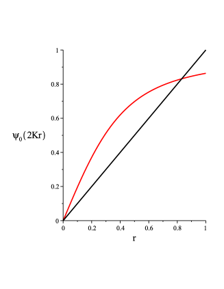
(a) Function $\Psi^{\mu}(2K\cdot)$ for $\mu=\delta_{0}$, $K=2$.

(b) Function $\Psi^{\mu}(2K\cdot)$ for $\mu=\frac{1}{2}\left(\delta_{-1}+\delta_{1}\right)$, $K=3.5$.

Figure 1. Plot of the fixed-point function $\Psi^{\mu}(2K\cdot)$ for two choices of $K$ and $\mu$. $\Psi^{\delta_{0}}(\cdot)$ is strictly concave with derivative at the origin equal to $1/2$ (Fig. 1a) but even for a simple instance of $\mu$ (Fig. 1b) concavity is lost and there are several non-trivial fixed-points, each of them corresponding to one circle of non trivial stationary solutions. Note that in the case of Fig. 1b, $K<\widetilde{K}=5$ so that the phase transition is not given by the derivative of $\Psi^{\mu}(2K\cdot)$ at the origin.

1.4. An overview of the results we present

Here are two natural questions:

• What are the stability properties of the non-trivial stationary solutions?

• What happens if $\mu$ is not symmetric?

Our work addresses these two questions and provides complete answers for weak disorder. The precise set-up of our work is better understood if we remark from now that we can assume $m_{\omega}:=\int\omega\mu(\,\text{\rm d}\omega)=0$. In fact, if this is not the case we can map the model to a model with $m_{\omega}=0$ by putting ourselves on the frame that rotates with speed $m_{\omega}$, that is if we consider the diffusion $\{\varphi^{\omega}_{j}(t)-m_{\omega}t\}_{j=1,\ldots,N}$. So, we assume henceforth $m_{\omega}=0$ and we rewrite the natural frequencies as $\delta\omega$, with $\delta$ a non-negative parameter. We assume moreover that

$$\operatorname*{Supp}(\mu)\subseteq[-1,1]\,.$$ (1.9)

In this set-up, (1.4) becomes

$$\partial_{t}p_{t}^{\delta}(\theta,\omega)\,=\,\frac{1}{2}\Delta p_{t}^{\delta}(\theta,\omega)-\partial_{\theta}\Big{(}p_{t}^{\delta}(\theta,\omega)(\langle J*p_{t}^{\delta}\rangle_{\mu}(\theta)+\delta\omega)\Big{)}\,.$$ (1.10)

Note that this leads to (obvious) changes to (1.5)-(1.7). We have introduced this parameterization because the results that we present are for small values of $\delta$. In particular we are going to show that for any $K>1$, there exists $\delta_{0}>0$ such that for $\delta\in[0,\delta_{0}]$

• there exists a solution $p_{t}^{\delta}(\theta,\omega)$ to (1.10) of the form $q(\theta-c_{\mu}(\delta)t)$, we show that $c_{\mu}(\delta)=O(\delta^{3})$ and we actually give an expression for $\lim_{\delta\searrow 0}c_{\mu}(\delta)/\delta^{3}$: this is a rotating wave (or limit-cycle) for the dynamical system (1.10) and we establish its stability under perturbations;

• when $\mu$ is symmetric and $K>\widetilde{K}$ we show that there is, up to rotation symmetry, only one non-trivial solution and that it is (linearly and non-linearly) stable.

The results we obtain are based on the rather good understanding that we have of the case $\delta=0$ that, as we have already explained, is reversible and the corresponding Fokker-Planck PDE is of gradient flow type (e.g. [15] and references therein). These properties have been exploited in [3] in order to extract a number of properties of the Fokker-Planck PDE (denoted from now on: reversible PDE)

$$\partial_{t}p_{t}(\theta)\,=\,\frac{1}{2}\Delta p_{t}(\theta)-\partial_{\theta}\Big{(}p_{t}(\theta)(J*p_{t})(\theta)\Big{)}\,,$$ (1.11)

and notably the linear stability of the non-trivial stationary solutions. In fact one can find in [3] an analysis of the evolution operator linearized around the non-trivial stationary solutions. Some of the results in [3] are recalled in the next section, but they are not directly applicable because the $\delta=0$ case that corresponds to what interests us is rather

$$\partial_{t}p_{t}(\theta,\omega)\,=\,\frac{1}{2}\Delta p_{t}(\theta,\omega)-\partial_{\theta}\Big{(}p_{t}(\theta,\omega)(\langle J*p_{t}\rangle_{\mu}(\theta)\Big{)}\,,$$ (1.12)

which we call non-disordered PDE. So the natural frequencies have no effective role beyond separating the various rotators into populations with given natural (ineffective) frequency that now are just labels. But in order to set-up a proper perturbation procedure we need to control (1.12) and, in particular, we need (and establish) a spectral gap inequality for the evolution (1.12) linearized around the non-trivial solutions.

This spectral analysis is going to be central both for the general and for the symmetric disorder case. In the general set-up we are going to exploit the normally hyperbolic structure [10, 18] of the manifold of stationary solutions of (1.12) and the robustness of such structures (like in [8]). In the case of symmetric $\mu$ we can get more precise results by ad hoc estimates, made possible by the explicit expressions (1.5)-(1.7), and use results in the general theory of operators [16] and perturbation theory of self-adjoint operators [12].

The normal hyperbolic manifold approach allows to treat cases that are substantially more general and notably the case of

$$\partial_{t}p_{t}(\theta,\omega)\,=\,\frac{1}{2}\Delta p_{t}(\theta,\omega)-\partial_{\theta}\Big{(}p_{t}(\theta,\omega)(\langle J*p_{t}\rangle_{\mu}(\theta)+\delta U(\theta,\omega))\Big{)}\,,$$ (1.13)

which is the large $N$ limit of (1.1) with the term $\omega_{j}\,\text{\rm d}t$ replaced by $U(\varphi^{\omega}_{j}(t),\omega_{j})\,\text{\rm d}t$, with $U\in C^{1}({\mathbb{S}}\times{\mathbb{R}};\,{\mathbb{R}})$. In this case each oscillator has its own non-trivial dynamics which may be very different from the dynamics of other oscillators: consider for example

$$U(\varphi,\omega)\,=\,b+\omega+a\sin(\varphi)\,,\ \ \ a,b\in{\mathbb{R}}\,,$$ (1.14)

and $\mu$ uniform over $[-1,1]$. For $a\in(-1,1)$ there are some active rotators [21, 8] that in absence of noise and interaction ($\sigma=K=0$) rotate (this happens if $|b+\omega|>|a|$ and of course the direction of rotation depends on the sign of $b+\omega$) and others that instead are stuck at a fixed point (this happens if $|b+\omega|\leq|a|$). Our approach allows us to establish that there is a synchronization regime for $K>1$ and $\delta$ small and to describe the dynamics of the system in this regime. This is going to be detailed in Section 5.

The two questions raised at the beginning of this section have been already repeatedly approached but looking at synchronized solutions as bifurcation from incoherence. The results are hence for $K$ close to the critical value corresponding to the breakdown of linear stability of $1/2\pi$: one can find a detailed review of the vast literature on this issue in [1, Sec. III]. Our results are instead for arbitrary $K>1$, but $\delta$ smaller than $\delta_{0}(K)$ and of course $\delta_{0}(K)$ vanishes as $K$ approaches $1$.

2. Mathematical set-up and main results

2.1. The reversible and the non-disordered PDE

We first recall some results about the reversible PDE (1.11). The stationary solutions $q_{0}(\theta)=q(\theta,0)$ are, up to rotation invariance, given by (1.5)-(1.7), but formulas get simpler, namely

$$q_{0}(\theta)\,=\,\frac{1}{Z_{0}(2Kr_{0})}\exp(2Kr_{0}\cos(\theta))\,,$$ (2.1)

where $Z_{0}(x):=Z(0,x)^{\frac{1}{2}}$ and this time we have the more explicit expression $Z_{0}(x)\,=\,\int_{{\mathbb{S}}}e^{x\cos(\theta)}\,\text{\rm d}\theta=2\pi I_{0}(x)$ is the normalization constant and $r_{0}$ is a solution of the fixed-point problem

$$r_{0}\,=\,\Psi_{0}(2Kr_{0})\qquad\text{where}\qquad\Psi_{0}(x)\,:=\,\frac{I_{1}(x)}{I_{0}(x)}\,,$$ (2.2)

where we used standard notations for the modified Bessel functions

$$I_{i}(x)\,=\,\frac{1}{2\pi}\int_{{\mathbb{S}}}(\cos(\theta))^{i}\exp(x\cos(\theta))\,\text{\rm d}\theta\,\qquad i=0,1\,.$$ (2.3)

The mapping $\Psi_{0}$ is increasing, concave (see [17]) and with derivative at $0$ equal to $\frac{1}{2}$. Consequently if $K\;\leqslant\;1$, $r_{0}=0$ is the unique solution of the fixed-point problem, and $q(\cdot)\equiv\frac{1}{2\pi}$ is the only stationary solution of (1.11). If $K>1$, we get in addition a circle (because of the rotation invariance) of nontrivial stationary solutions

$$M_{\text{rev}}\,:=\,\{q_{\psi,0}(\cdot):=q_{0}(\cdot-\psi):\,\psi\in{\mathbb{S}}\}\qquad\text{with}\qquad q_{0}(\theta)\,:=\,\frac{\exp(2Kr_{0}\cos(\theta))}{\int_{{\mathbb{S}}}\exp(2Kr_{0}\cos(\theta))}$$ (2.4)

where $r_{0}=r_{0}(K)$ is the unique non trivial fixed-point (2.2).

Let us now focus on the non-disordered PDE (1.12) and let us insist on the fact that we are interested in solutions such that $\varphi^{\delta}_{t}(\cdot,\omega)$ is a probability density. Observe then that if $q(\theta,\omega)$ is a stationary solution of (1.12), we see (Appendix A) that $q$ is $C^{\infty}$ with respect to $\theta$ and that $\langle q\rangle_{\mu}$ is a stationary solution for (1.11). So there exists $\psi\in{\mathbb{S}}$ such that $\langle q\rangle_{\mu}=q_{\psi}$ and a short computation leads to

$$\langle J*q\rangle_{\mu}(\theta)\,=\,-K\sin(\theta-\psi)\,,$$ (2.5)

and, since $\int_{{\mathbb{S}}}q(\theta,\omega)\,\text{\rm d}\theta=1$ for almost all $\omega$, we obtain that $q(\cdot,\omega)=q_{\psi}(\cdot)$ for almost all $\omega$. In conclusion, with some abuse of notation, we can say the stationary solutions of (1.11) and (1.12) are the same: of course in the second case the function space includes the dependence on $\omega$, so we choose a different notation, that is $M_{0}$, for the corresponding circle of non-trivial stationary solutions.

An important issue for us is the stability of $M_{0}$ (for its existence we are assuming $K>1$) and for this we denote by $A$ the linearized evolution operator of (1.12) around $q_{0}$

$$Au(\theta,\omega)\,:=\,\frac{1}{2}\Delta u(\theta,\omega)-\partial_{\theta}\Big{(}q_{0}(\theta)\langle J*u\rangle_{\mu}(\theta)+u(\theta,\omega)J*q_{0}(\theta)\Big{)}$$ (2.6)

with domain

$${\mathcal{D}}(A)\,:=\,\left\{u\in C^{2}({\mathbb{S}}\times{\mathbb{R}},{\mathbb{R}}):\,\int_{{\mathbb{S}}}u(\theta,\omega)\,\text{\rm d}\theta=0\,\text{ for all }\omega\right\}\,.$$ (2.7)

For any smooth positive function $k:{\mathbb{S}}\mapsto{\mathbb{R}}$, we introduce the Hilbert space $H^{-1}_{k,\mu}$ defined by the closure of ${\mathcal{D}}(A)$ for the norm $\|\cdot\|_{-1,k,\mu}$ associated with the scalar product

$$\langle u,\,v\,\rangle_{-1,k,\mu}\,:=\,\int_{{\mathbb{R}}\times{{\mathbb{S}}}}\frac{{\mathcal{U}}(\theta,\omega){\mathcal{V}}(\theta,\omega)}{k(\theta)}\,\text{\rm d}\theta\mu(\,\text{\rm d}\omega),$$ (2.8)

where $\omega$ a.s., ${\mathcal{U}}(\cdot,\omega)$ is the primitive of $u(\cdot,\omega)$ such that $\int_{{\mathbb{S}}}\frac{{\mathcal{U}}(\theta,\omega)}{k(\theta)}\,\text{\rm d}\theta=0$, and ${\mathcal{V}}(\cdot,\omega)$ is defined in the analogous fashion. Let us remark (see [8, Sec. 2]) immediately that

$$\|u\|_{-1,k_{1},\mu}^{2}\,\;\leqslant\;\,\frac{\|k_{2}\|_{\infty}}{\|k_{1}\|_{\infty}}\|u\|_{-1,k_{2},\mu}^{2}\,,$$ (2.9)

so that all the norms we have introduced are equivalent. For the case $k(\cdot)\equiv 1$ we use the notations $H^{-1}_{\mu}$ and $\|\cdot\|_{-1,\mu}$. We will prove the following result, which is just technical, but it will be of help to understand our main results:

Proposition 2.1.

A is essentially self-adjoint in $H^{-1}_{{q_{0}},\mu}$. Moreover the spectrum lies in $(-\infty,0]$, $0$ is a simple eigenvalue, with eigenspace spanned by $\partial_{\theta}q_{0}$, and there is a spectral gap, that is the distance $\lambda_{K}$ between $0$ and the rest of the spectrum is positive.

The proof of this result builds on [3, Th. 1.8] that deals with the reversible case and the (lower) bound on the spectral gap $\lambda_{K}$ that we obtain coincides with the quantity $\lambda(K)$ in [3, Th. 1.8] (this bound can be improved as explained in in [3, Sec. 2.5] and sharp estimates on the spectral gap can be obtained in the limit $K\searrow 1$ and $K\nearrow\infty$). For the reversible evolution, the linear operator $L_{q_{0}}$ is defined by

$$L_{q_{0}}u(\theta)\,:=\,\frac{1}{2}\Delta u(\theta)-\partial_{\theta}\Big{(}q_{0}(\theta)J*u(\theta)+u(\theta)J*q_{0}(\theta)\Big{)},$$ (2.10)

with domain $D(L_{q_{0}})$ given by the $C^{2}({\mathbb{S}},{\mathbb{R}})$ functions with zero integral.

2.2. Synchronization: the main result without symmetry assumption

Proposition 2.1 is a key ingredient for our main results and the functional space $H^{-1}$ appears in it, but an important role is played also by $L^{2}(\lambda\otimes\mu)$, $\lambda$ is the Haar measure on ${\mathbb{S}}$, whose norm is denoted by $\|\,\cdot\,\|_{2,\mu}$. For $C>0$ and $M\subset L^{2}(\lambda\otimes\mu)$ we set ${\mathcal{N}}_{2,\mu}(M,C):=\{u:\,$there exists $v\in M$ such that $\|u-v\|_{2,\mu}\leq C\}$. In the statement below $q\in M_{0}$ is the element of the manifold such that $q(\cdot,\omega)=q_{0}(\cdot)$, cf. (2.1), with $r_{0}(K)>0$ (hence $K>1$).

Theorem 2.2.

For every $K>1$ there exists $\delta_{0}=\delta_{0}(K)>0$ such that for $|\delta|\leq\delta_{0}$ there exists $\widetilde{q}_{\delta}\in L^{2}(\lambda\otimes\mu)$, satisfying $\|\widetilde{q}_{\delta}-q\|_{2,\mu}=O(\delta)$ and a value $c_{\mu}(\delta)\in{\mathbb{R}}$ such that if we set

$$q^{(\psi)}_{t}(\theta,\omega)\,:=\,\widetilde{q}_{\delta}(\theta-c_{\mu}(\delta)t-\psi)\,,$$ (2.11)

then $q^{(0)}_{t}$ solves (1.10). Moreover

1. the family of solutions $\{q^{(\psi)}_{\cdot}\}_{\psi}$ is stable in the sense that there exist two positive constants $\beta=\beta(K)$ and $C=C(K)$ such that if $p_{0}^{\delta}\in{\mathcal{N}}_{2,\mu}(M_{0},\delta)$, and $\int_{\mathbb{S}}p_{0}^{\delta}(\theta,\omega)\,\text{\rm d}\theta=0$ $\mu(\,\text{\rm d}\omega)$-a.s., then there exists $\psi_{0}\in{\mathbb{S}}$ such that for all $t\geq 0$

   $$\|q_{t}^{(\psi_{0})}-p_{t}^{\delta}\|_{2,\mu}\,\leq\,2C\exp(-\beta t)\,.$$ (2.12)

2. we have

   $$c_{\mu}(\delta)\,=\,\delta^{3}\frac{\left\langle\omega\partial_{\theta}n^{(2)},\partial_{\theta}q_{0}\right\rangle_{-1,{q_{0}},\mu}}{\left\langle\partial_{\theta}q_{0},\partial_{\theta}q_{0}\right\rangle_{-1,{q_{0}}}}+O(\delta^{5})\,,$$ (2.13)

   where $n^{(2)}$ is the unique solution of

   $$An^{(2)}\,=\,\omega\partial_{\theta}n^{(1)}\quad\text{ and }\quad\left\langle n^{(2)},\partial_{\theta}q_{0}\right\rangle_{-1,{q_{0}},\mu}\,=\,0\,,$$ (2.14)

   and $n^{(1)}$ is the unique solution of

   $$An^{(1)}\,=\,\omega\,\partial_{\theta}q_{0}\quad\text{ and }\quad\left\langle n^{(1)}\,,\,\partial_{\theta}q_{0}\right\rangle_{-1,{q_{0}},\mu}\,=\,0\,.$$ (2.15)

In the proof of Theorem 2.2 one finds also further estimates, in particular (see (4.19)) that one has

$$\widetilde{q}_{\delta}\,=\,q_{0}+\delta n^{(1)}+\delta^{2}n^{(2)}+O_{L^{2}}(\delta^{3})\,.$$ (2.16)

Actually, see Remark 4.2, the argument of proof can be pushed farther to obtain arbitrarily many terms in development (2.16), as well as in

$$c_{\mu}(\delta)\,=\,c_{3}\delta^{3}+c_{5}\delta^{5}+\ldots\,.$$ (2.17)

In Table 1 we report a comparison between the $c_{\mu}(\delta)$ obtained by solving numerically (1.10) and by evaluating the leading order $c_{3}$, i.e. by using (2.13).

m $\delta$	$K=2$	$K=1.5$	$K=1.1$
$0.5$	$-1.56300\cdot 10^{-2}$	$-8.59626\cdot 10^{-2}$	$-3.01064\cdot 10^{-1}$
$0.1$	$-1.23998\cdot 10^{-2}$	$-6.84835\cdot 10^{-2}$	$-2.72117\cdot 10^{-1}$
$0.05$	$-1.23072\cdot 10^{-2}$	$-6.79553\cdot 10^{-2}$	$-2.69460\cdot 10^{-1}$
$0.01$	$-1.22776\cdot 10^{-2}$	$-6.77921\cdot 10^{-2}$	$-2.68603\cdot 10^{-1}$
$0.005$	$-1.22767\cdot 10^{-2}$	$-6.77869\cdot 10^{-2}$	$-2.68576\cdot 10^{-1}$
$c_{3}$	$-1.22764\cdot 10^{-2}$	$-6.77851\cdot 10^{-2}$	$-2.68567\cdot 10^{-1}$

Table 1. For the case $\mu=p\delta_{1-p}+(1-p)\delta_{-p}$, $p=0.2$, we have computed (numerically) $c_{\mu}(\delta)/\delta^{3}$ for three values of $K$ and five values of $\delta$. In the last line we report the value $c_{3}=\lim_{\delta\searrow 0}c_{\mu}(\delta)/\delta^{3}$ that one obtains by using (2.13).

2.3. Symmetric disorder case

Let us focus on the case in which the distribution of the disorder $\mu$ is symmetric. In this case, at least for small disorder, Theorem 2.2 is just telling us that the leading order in the development for the speed $c_{\mu}(\delta)$ is zero: one can actually work harder and show that such a development yields zero terms to all orders. In reality in this case we already know, see (1.5)-(1.7), that for $K$ sufficiently large there is at least a non-trivial stationary profile, hence, by rotation symmetry, at least one whole circle of stationary solutions. Actually, we can show that for $\delta$ small there is just one circle, that we call $M_{\delta}$, of non-trivial stationary solutions and this circle converges to $M_{0}$ as $\delta\searrow 0$ (in $C^{j}$, for every $j$) so the rotating solutions found in Theorem 2.2 must be the stationary solutions in $M_{\delta}$.

In order to be precise about this issue, we point out that (1.5)-(1.7) are written for (1.4) while we work rather with (1.10). The changes are obvious, but we introduce a notation for the analog of (1.7):

$$r_{\delta}\,=\,\Psi_{\delta}^{\mu}(2Kr_{\delta}),\qquad\text{where,}\,\Psi_{\delta}^{\mu}(x)\,:=\,\int_{{\mathbb{R}}}\frac{\int_{{\mathbb{S}}}\cos(\theta)S(\theta,\delta\omega,x)\,\text{\rm d}\theta}{Z(\delta\omega,x)}\mu(\,\text{\rm d}\omega)\,.$$ (2.18)

Lemma 2.3.

For all $K_{\min}<K_{\max}$, there exists $\delta_{1}=\delta_{1}(K_{\min},K_{\max})>0$ such that, for all $0<K_{\min}<K<K_{\max}$ and all $\delta\;\leqslant\;\delta_{1}$ the function $\Psi_{\delta}^{\mu}$ is strictly concave on $[0,1]$. Therefore for (1.7) has only a positive solution $r_{\delta}=r_{\delta}(K,\mu)$. Moreover $\lim_{\delta\searrow 0}r_{\delta}=r_{0}$.

We point out that in spite of the fact that $\Psi^{\mu}$ is explicit (cf. (2.2)), it is not so straightforward to show that it is concave. We show that $\Psi_{\delta}^{\mu}$ remains strictly concave for a small $\delta$ via a perturbation argument. But the conjecture (see [11] and [5]) that $\Psi^{\mu}$ is strictly concave for unimodal distributions $\mu$ is still an open issue.

Remark 2.4.

A direct computation shows that the derivative of $\Psi^{\mu}_{\delta}$ at the origin is $1/(2\widetilde{K}_{\delta})$, for $\widetilde{K}_{\delta}\,:=\,\left(\int_{{\mathbb{R}}}\frac{\mu(\,\text{\rm d}\omega)}{1+4\delta^{2}\omega^{2}}\right)^{-1}$ (of course $\widetilde{K}_{1}$ coincides with $\widetilde{K}$, introduced in (1.8)). Under the hypothesis of Lemma 2.3, one therefore sees that there is a synchronization transition at $K=\widetilde{K}_{\delta}$ in the sense that for $K\leq\widetilde{K}_{\delta}$ the only stationary solution is $\frac{1}{2\pi}$ while for $K>\widetilde{K}_{\delta}$ also the manifold of non-trivial stationary solutions appears (and there is no other stationary solution).

Theorem 2.2 provides a stability statement for $M_{\delta}$. This result can be sharpened and for this let us introduce the linear operator

$$L^{\omega}_{{q}}u(\theta,\omega)\,:=\,\frac{1}{2}\Delta u(\theta,\omega)-\partial_{\theta}\left(u(\theta,\omega)\left(\langle J\ast{q}\rangle_{\mu}(\theta)+\delta\omega\right)+{q}(\theta,\delta\omega)\langle J\ast u\rangle_{\mu}(\theta)\right),$$ (2.19)

The domain ${\mathcal{D}}(L^{\omega}_{{q}})$ of the operator $L^{\omega}_{{q}}$ is chosen to be the same as for $A$, cf. (2.7).

We place ourselves within the framework of Lemma 2.3, in the sense that $\delta$ is small enough to ensure the uniqueness of a non-trivial stationary solution (of course existence requires $K>\widetilde{K}_{\delta}$ and this is implied by $K>1$ if $\delta$ is sufficiently small). We prove a number of properties of the linear operator (2.19), saying notably that it has a simple eigenvalue at zero and the rest of spectrum is at a positive distance from zero and it is in a cone in that lies in the negative complex half plane. We summarize in the next statement the qualitative features of our results on $L_{q}^{\omega}$, but what we really prove are quantitative explicit estimates: the interested reader finds them in Section 6.

Theorem 2.5.

The operator $L^{\omega}_{{q}}$ has the following spectral properties: $0$ is a simple eigenvalue for $L^{\omega}_{{q}}$, with eigenspace spanned by $(\theta,\omega)\mapsto q^{\prime}(\theta,\omega)$. Moreover, for all $K>1$, $\rho\in(0,1)$, $\alpha\in(0,\pi/2)$, there exists $\delta_{2}=\delta_{2}(K,\rho,\alpha)$ such that for all $0\;\leqslant\;\delta\;\leqslant\;\delta_{2}$, the following is true:

• $L^{\omega}_{{q}}$ is closable and its closure has the same domain as the domain of the self-adjoint extension of $A$;

• The spectrum of $L^{\omega}_{{q}}$ lies in a cone $C_{\alpha}$ with vertex $0$ and angle $\alpha$

  $$C_{\alpha}\,:=\,\left\{\lambda\in{\mathbb{C}}\,;\,\frac{\pi}{2}+\alpha\;\leqslant\;\arg(\lambda)\;\leqslant\;\frac{3\pi}{2}-\alpha\right\}\subseteq\left\{z\in{\mathbf{C}}\,;\,\Re(z)\;\leqslant\;0\right\}\,;$$ (2.20)

• There exists $\alpha^{\prime}\in(0,\frac{\pi}{2})$ such that $L^{\omega}_{{q}}$ is the infinitesimal generator of an analytic semi-group defined on a sector $\{\lambda\in{\mathbb{C}},\,|\arg(\lambda)|<\alpha^{\prime}\}$;

• The distance between $0$ and the rest of the spectrum is strictly positive and is at least equal to $\rho\lambda_{K}$, where $\lambda_{K}$ is the spectral gap of the operator $A$ introduced in Proposition 2.1.

2.4. Organization of remainder of the paper

In Section 3 we introduce the notion of stable normally hyperbolic manifold, we recall its robustness properties, and show that $M_{0}$ is in this class of manifolds. The essential ingredient is Proposition 2.1 that, directly or indirectly, plays a role in each subsequent section. Section 3 is also devoted to the proof of Proposition 2.1. The proof of Theorem 2.2 is then completed in Section 4, that is mainly devoted to perturbation arguments. The case of the active rotators is treated in Section 5, while Section 6 deals with the case symmetric disorder distribution and, notably, with the proof of Theorem 2.5 and of a number of related quantitative estimates.

3. Hyperbolic structures and periodic solutions

In this section we present the arguments proving the existence of the periodic solution of Theorem 2.2. We rely on the fact that the circle of stationary solutions $M_{0}$ is a stable normally hyperbolic manifold, and on the robustness of this kind of structure : adding the perturbation term $-\delta\partial_{\theta}(p_{t}(\theta,\omega)\omega)$ in (1.12), this manifold $M_{0}$ is deformed into another manifold $M_{\delta}$, and thanks to the rotation invariance of the problem, $M_{\delta}$ is a circle too. The spectral gap of operator $A$ (Property 2.1) which induces the hyperbolic property of $M_{0}$ is proved at the end of this section.

3.1. Stable normally hyperbolic manifolds

We start by quickly reviewing the notion of of stable normally hyperbolic manifold (SNHM). The evolution of (1.10) will be studied in the space $X^{1}_{\mu}$ defined by

$$X^{1}_{\mu}\,:=\,\left\{u\in L^{2}(\lambda\otimes\mu),\,\int_{{\mathbb{S}}}u(\theta,\omega)\,\text{\rm d}\theta=1\quad\omega\text{ a.s.}\right\}$$ (3.1)

where $\lambda$ denotes the Lebesgue measure on ${\mathbb{S}}$. This is made possible by the conservative character of the dynamics. The $L^{2}$-norm with respect to the measure $\lambda\otimes\mu$ will be denoted by $\|\cdot\|_{2,\mu}$. We will also use the space $X^{0}_{\mu}$ defined by

$$X^{0}_{\mu}\,:=\,\left\{u\in L^{2}(\lambda\otimes\mu),\,\int_{{\mathbb{S}}}u(\theta,\omega)\,\text{\rm d}\theta=0\quad\omega\text{ a.s.}\right\}\,.$$ (3.2)

To define a SNHM, we need a dynamics: we have in mind (1.10) but for the moment let us just think of an evolution semigroup in $X^{1}_{\mu}$ that gives rise to $\{u_{t}\}_{t\geq 0}$, with $u_{0}=u$, to which we can associate a linear evolution semigroup $\{\Phi(u,t)\}_{t\geq 0}$ in $X^{0}_{\mu}$, satisfying $\partial_{t}\Phi(u,t)v=L(t)\Phi(u,t)v$ and $\Phi(u,0)v=v$, where $L(t)$ is the operator obtained by linearizing the evolution around $u_{t}$.

For us a SNHM $M\subset X^{1}_{\mu}$ (in reality we are interested only in $1$-dimensional manifolds, that is curves, but at this stage this does not really play a role) of characteristics $\lambda_{1}$, $\lambda_{2}$ ($0\leq\lambda_{1}<\lambda_{2}$) and $C>0$ is a $C^{1}$ compact connected manifold which is invariant under the dynamics and for every $u\in M$ there exists a projection $P^{o}(u)$ on the tangent space of $M$ at $u$, that is ${\mathcal{R}}(P^{o}(u))=:T_{u}M$, which, for $v\in L^{2}_{0}$, satisfies the following properties:

1. for every $t\geq 0$ we have

   $$\Phi(u,t)P^{o}(u_{0})v\,=\,P^{o}(u_{t})\Phi(u,t)v\,,$$ (3.3)

2. we have

   $$\|\Phi(u,t)P^{o}(u_{0})v\|_{2,\mu}\,\leq\,C\exp(\lambda_{1}t)\|v\|_{2,\mu}\,,$$ (3.4)

   and, for $P^{s}\,:=\,1-P^{o}$, we have

   $$\|\Phi(u,t)P^{s}(u_{0})v\|_{2,\mu}\,\leq\,C\exp(-\lambda_{2}t)\|v\|_{2,\mu}\,,$$ (3.5)

   for every $t\geq 0$;

3. there exists a negative continuation of the dynamics $\{u_{t}\}_{t\leq 0}$ and of the linearized semigroup $\{\Phi(u,t)P^{o}(u_{0})v\}_{t\leq 0}$ and for any such continuation we have

   $$\|\Phi(u,t)P^{o}(u_{0})v\|_{2,\mu}\,\leq\,C\exp(-\lambda_{1}t)\|v\|_{2,\mu}\,,$$ (3.6)

   for $t\leq 0$.

3.2. $M_{0}$ is a SNHM

First of all: the dynamics on $M_{0}$ is trivial. For $q_{\psi}\in M_{0}$, the projection $P^{o}_{q_{\psi}}$ on the tangent space is the projection on the subspace spanned by $q^{\prime}_{\psi}$:

$$P^{o}_{q_{\psi}}u\,=\,\frac{\left\langle u,q^{\prime}_{\psi}\right\rangle_{-1,q_{\psi},\mu}}{\left\langle q^{\prime}_{\psi},q^{\prime}_{\psi}\right\rangle_{-1,q_{\psi}}}q^{\prime}_{\psi}$$ (3.7)

and since the dynamic on the manifold is trivial, we are allowed to choose for the parameters $\lambda_{1}=0$ and $\lambda_{2}=\lambda_{K}$ (where we recall that $\lambda_{K}$ is given by Proposition 2.1).

We are in the same situation as in [8]. For a suitable perturbation and if $\delta$ is small enough, the circle $M_{0}$ is smoothly transformed into another SNHM $M_{\delta}$, which is close to $M_{0}$. The proof is the same as in [8, Sec. 5], which, in turn builds on results in [18]): the spaces we are working in are more general since we have to deal with the disorder. Here suitable perturbation means being an element of $C^{1}(X^{0}_{\mu},H^{-1}_{\mu})$, but it is clearly the case for the perturbation $u\mapsto-\delta\,\omega\,\partial_{\theta}u$ when $\mu$ is of compact support. The following theorem works for all $C^{1}(X^{0}_{\mu},H^{-1}_{\mu})$ perturbations:

Theorem 3.1.

[8, Sec. 5] For every $K>1$ there exists $\delta_{0}>0$ such that if $\delta\in[0,\delta_{0}]$ there exists a stable normally hyperbolic manifold $M_{\delta}$ in $X^{1}_{\mu}$ for the perturbed equation (1.10). Moreover we can write

$$M_{\delta}\,=\,\left\{q_{\psi}+\phi_{\delta}\left(q_{\psi}\right):\,\psi\in{\mathbb{S}}\right\}\,,$$ (3.8)

for a suitable function $\phi_{\delta}\in C^{1}(M_{0},X^{0}_{\mu})$ with the properties that

• $\phi_{\delta}(q)\in{\mathcal{R}}(A)$;

• there exists $C>0$ such that $\sup_{\psi}(\|\phi_{\delta}\left(q_{\psi}\right)\|_{2,\mu}+\|\partial_{\psi}\phi_{\delta}(q_{\psi})\|_{2,\mu})\leq C\delta$.

Remark 3.2.

A byproduct of the proof in [8, Sec. 5] is also that $M_{\delta}$ is the unique invariant manifold in a $L^{2}(\lambda,\mu)$-neighborhood of $M_{0}$. So in the case of (1.10), thanks to the symmetry of the problem that tells us that any rotation of $M_{\delta}$ is still a invariant manifold, $M_{\delta}$ is in fact a circle, and that the dynamics on this circle is a traveling wave of constant (possibly zero) speed $c_{\mu}(\delta)$. So the invariant manifold we get for (1.10) is even $C^{\infty}$. In this sense, when dealing with (1.10), we are using only part of the strength of Theorem 3.1. Of course this symmetry argument does not apply when dealing with (1.13).

Remark 3.3.

Theorem 3.1 addresses the existence and the linear stability of the manifold $M_{\delta}$. The non-linear stability statement in Theorem 2.2(1) follows from Theorem 3.1 combined with [9, Theorem 8.1.1], when the dynamics is periodic with non zero speed on $M_{\delta}$. If $M_{\delta}$ is a manifold of stationary points, the argument for the non-linear stability follows by repeating the argument in [7, Th. 4.8], where the non-disordered case is treated.

We now prove Proposition 2.1 and thus that $M_{0}$ is a SNHM.

3.3. The spectral gap estimate (proof of Proposition 2.1)

We start by remarking that $A$ is symmetric for the scalar product $\left\langle\cdot\,,\,\cdot\right\rangle_{-1,{q_{0}},\mu}$ (recall (2.8)). In fact, for $u$ and $v$ in ${\mathcal{D}}(A)$, a short computation gives (in the following we use the notation $u^{\prime}(\theta,\omega)=\partial_{\theta}u(\theta,\omega)$)

$$\left\langle v\,,\,Au\right\rangle_{-1,{q_{0}},\mu} \,=\,\int_{{\mathbb{R}}\times{{\mathbb{S}}}}\left[\frac{{\mathcal{V}}(\theta,\omega)}{q_{0}(\theta)}\left(\frac{u^{\prime}(\theta,\omega)}{2}-u(\theta,\omega)J*q_{0}(\theta)-q_{0}(\theta)\langle J*u\rangle_{\mu}(\theta)\right)\right]\,\text{\rm d}\theta\,\text{\rm d}\mu$$ (3.9)

$$\,=\,-\frac{1}{2}\int_{{\mathbb{R}}\times{{\mathbb{S}}}}\frac{u(\theta,\omega)v(\theta,\omega)}{q_{0}(\theta)}\,\text{\rm d}\theta\,\text{\rm d}\mu+\int_{{\mathbb{R}}}\int_{({\mathbb{S}})^{2}}v(\theta,\omega)\widetilde{J}*u(\theta,\omega^{\prime})\,\text{\rm d}\theta\,\text{\rm d}\mu\otimes\mu\,,$$

where $\widetilde{J}(\theta)=K\cos(\theta)$. We now first prove an inequality for $A$ that is stronger than the spectral gap inequality and then deduce that $A$ is (essentially) self-adjoint. We define the two following scalar products, which were used for the non-disordered case in [3]:

$$\left\langle u\,,\,v\right\rangle_{-1,{q_{0}}}\,:=\,\int_{{\mathbb{S}}}\frac{{\mathcal{U}}(\theta){\mathcal{V}}(\theta)}{q_{0}(\theta)}\,\text{\rm d}\theta\,,$$ (3.10)

where ${\mathcal{U}}(\cdot)$ is the primitive of $u(\cdot)$ such that $\int_{{\mathbb{S}}}\frac{{\mathcal{U}}(\theta)}{q_{0}(\theta)}\,\text{\rm d}\theta=0$ and

$$\left\langle u\,,\,v\right\rangle_{2,q_{0}}\,:=\,\int_{{\mathbb{S}}}\frac{u(\theta)v(\theta)}{q_{0}(\theta)}\,\text{\rm d}\theta\,.$$ (3.11)

We denote the closures of ${\mathcal{D}}(L_{0})$ for these scalar products respectively by $H^{-1}_{{q_{0}}}$ and $L^{2}_{{q_{0}}}$. In the disordered case, $L^{2}_{{q_{0}}}$ corresponds to the space $L^{2}_{{q_{0}},\mu}$, which we define by the closure of ${\mathcal{D}}(A)$ with respect to the norm $\|\cdot\|_{2,{q_{0}},\mu}$ associated with the scalar product

$$\left\langle u\,,\,v\right\rangle_{2,{q_{0}},\mu}\,:=\,\int_{{\mathbb{R}}}\int_{{\mathbb{S}}}\frac{u(\theta,\omega)v(\theta,\omega)}{q_{0}(\theta)}\,\text{\rm d}\theta\,\text{\rm d}\mu\,.$$ (3.12)

The two Dirichlet forms for the disordered and non-disordered case are respectively

$${\mathcal{E}}_{\mu}(u)\,=\,-\left\langle Au\,,\,u\right\rangle_{-1,{q_{0}},\mu}\,,$$ (3.13)

and

$${\mathcal{E}}(u)\,=\,-\left\langle L_{q_{0}}u\,,\,u\right\rangle_{-1,{q_{0}}}\,.$$ (3.14)

As in [3], we first prove a spectral gap type inequality that involves the scalar product $\left\langle\cdot\,,\,\cdot\right\rangle_{2,q_{0}}$. For this we introduce the projections on the line spanned by $q^{\prime}_{0}$ in the spaces $L^{2}_{{q_{0}},\mu}$ and $L^{2}_{{q_{0}}}$

$$P_{2,{q_{0}},\mu}u=\frac{\left\langle u\,,\,q^{\prime}_{0}\right\rangle_{2,{q_{0}},\mu}}{\left\langle q^{\prime}_{0}\,,\,q^{\prime}_{0}\right\rangle_{2,{q_{0}}}}q^{\prime}_{0}\qquad\text{for all}\,u=u(\theta,\omega)\in L^{2}_{{q_{0}},\mu}\,,$$ (3.15)

and

$$P_{2,{q_{0}}}u\,=\,\frac{\left\langle u\,,\,q^{\prime}_{0}\right\rangle_{2,{q_{0}}}}{\left\langle q^{\prime}_{0}\,,\,q^{\prime}_{0}\right\rangle_{2,{q_{0}}}}q^{\prime}_{0}\qquad\text{for all}\ u\in L^{2}_{{q_{0}}}\,.$$ (3.16)

Remark that since $q^{\prime}_{0}$ does not depend on $\omega$,

$$\left\langle q^{\prime}_{0}\,,\,q^{\prime}_{0}\right\rangle_{2,{q_{0}},\mu}\,=\,\left\langle q^{\prime}_{0}\,,\,q^{\prime}_{0}\right\rangle_{2,{q_{0}}}\quad\text{ and }\quad\left\langle q^{\prime}_{0}\,,\,q^{\prime}_{0}\right\rangle_{-1,{q_{0}},\mu}\,=\,\left\langle q^{\prime}_{0}\,,\,q^{\prime}_{0}\right\rangle_{-1,{q_{0}}}\,,$$ (3.17)

and that for all $u\in L^{2}_{{q_{0}},\mu}$

$$P_{2,{q_{0}},\mu}u\,=\,\langle P_{2,{q_{0}}}u\rangle_{\mu}\,=\,P_{2,{q_{0}}}\langle u\rangle_{\mu}\,.$$ (3.18)

Proposition 3.4.

For all $u\in L^{2}_{{q_{0}},\mu}$ such that for almost every $\omega$, $\int_{{\mathbb{S}}}u(\cdot,\omega)=0$

$${\mathcal{E}}_{\mu}(u)\,\;\geqslant\;\,c_{K}\left\langle u-P_{2,{q_{0}},\mu}u\,,\,u-P_{2,{q_{0}},\mu}u\right\rangle_{2,{q_{0}},\mu}\,,$$ (3.19)

with

$$c_{K}\,=\,1-K(1-r_{0}^{2})\in(0,1/2)\,.$$ (3.20)

The proof of this proposition relies on the corresponding result for the non-disordered case.:

Proposition 3.5.

(see [3, Prop. 2.3]) For all $u\in L^{2}_{{q_{0}}}$ such that for almost every $\omega$, $\int_{{\mathbb{S}}}u(\cdot,\omega)=0$

$${\mathcal{E}}(v)\,\;\geqslant\;\,c_{K}\left\langle u-P_{2,{q_{0}}}u\,,\,u-P_{2,{q_{0}}}u\right\rangle_{2,{q_{0}}}\,.$$ (3.21)

Proof of Proposition (3.4). The first step of the proof is to make the Dirichlet form of the non-disordered case appear in the the disordered case one, that is

$${\mathcal{E}}_{\mu}(u) \,=\,\langle{\mathcal{E}}(u)\rangle_{\mu}+\int_{{\mathbb{R}}}\int_{({\mathbb{S}})^{2}}u(\theta,\omega)\widetilde{J}*[u(\theta,\omega)-u(\theta,\omega^{\prime})]\,\text{\rm d}\theta\,\text{\rm d}\mu\otimes\mu$$ (3.22)

$$\,=\,\langle{\mathcal{E}}(u)\rangle_{\mu}+\frac{1}{2}\int_{{\mathbb{R}}}\int_{({\mathbb{S}})^{2}}[u(\theta,\omega)-u(\theta,\omega^{\prime})]\widetilde{J}*[u(\theta,\omega)-u(\theta,\omega^{\prime})]\,\text{\rm d}\theta\,\text{\rm d}\mu\otimes\mu\,,$$ (3.23)

and from Proposition (3.5) we see that

$$\langle{\mathcal{E}}(u)\rangle_{\mu}\,\;\geqslant\;\,c_{K}\left\langle u-P_{2,{q_{0}}}u\,,\,u-P_{2,{q_{0}}}u\right\rangle_{2,{q_{0}}}\,.$$ (3.24)

Now remark that if we define

$$v\,=\,u-P_{2,{q_{0}},\mu}u\,,$$ (3.25)

using (3.18) we get

$$v-P_{2,{q_{0}}}v\,=\,u-P_{2,{q_{0}}}u\,,$$ (3.26)

and so

$$\langle{\mathcal{E}}(u)\rangle_{\mu}\,\;\geqslant\;\,c_{K}\left\langle v-P_{2,{q_{0}}}v\,,\,v-P_{2,{q_{0}}}v\right\rangle_{2,{q_{0}},\mu}\,.$$ (3.27)

We now introduce an orthogonal decomposition of the space $L^{2}_{{q_{0}}}$ which is well adapted to the convolution with $\widetilde{J}$.

Lemma 3.6.

(See [3, Lemma 2.1].) We have the following decomposition

$$L^{2}_{{q_{0}}}\,=\,F_{0}\oplus^{\bot}F_{1/2}\oplus^{\bot}F_{K-1/2}$$ (3.28)

where

$$F_{0}\,:=\,\left\{\theta\mapsto a_{0}+\sum_{j\;\geqslant\;2}a_{j}\cos(j\theta)+b_{j}\sin(j\theta)\,;\,\sum_{j}a_{j}^{2}+b^{2}_{j}<\infty\right\}$$ (3.29)

and both $F_{1/2}$ and $F_{K-1/2}$ are one dimensional subspaces generated respectively by $\theta\mapsto\sin(\theta)q(\theta)\,(=-q^{\prime}_{0}(\theta)/2Kr_{0})$ and by $\theta\mapsto\cos(\theta)q_{0}(\theta)$. Moreover, when $u\in F_{\lambda}$, then

$$\widetilde{J}*u\,=\,\frac{\lambda}{q_{0}}u\,.$$ (3.30)

With the help of Lemma 3.6 we can find a lower bound for the last term in (3.23): choose $\alpha$ such that $P_{2,{q_{0}}}u=\alpha q^{\prime}_{0}$, so that we can write

$${\mathcal{E}}_{\mu}(u)\,\;\geqslant\;\,c_{K}\left\langle v-P_{2,{q_{0}}}v\,,\,v-P_{2,{q_{0}}}v\right\rangle_{2,{q_{0}},\mu}+\frac{\left\langle q^{\prime}_{0}\,,\,q^{\prime}_{0}\right\rangle_{2,{q_{0}}}}{4}\int_{({\mathbb{S}})^{2}}(\alpha(\omega)-\alpha(\omega^{\prime}))^{2}\,\text{\rm d}\mu\otimes\mu\,.$$ (3.31)

But if $P_{2,{q_{0}}}v=\beta q^{\prime}_{0}$ (recall that $v=u-P_{2,{q_{0}},\mu}u$), then since $P_{2,{q_{0}},\mu}u$ is colinear to $q^{\prime}_{0}$, for almost all $\omega$, $\omega^{\prime}$

$$\beta(\omega)-\beta(\omega^{\prime})\,=\,\alpha(\omega)-\alpha(\omega^{\prime})$$ (3.32)

and since $v$ is orthogonal to $q^{\prime}_{0}$ (with respect to $\langle\cdot,\cdot\rangle_{2,q_{0},\mu}$) we get

$$\int_{{\mathbb{R}}}\beta(\omega)\,\text{\rm d}\mu\,=\,0\,.$$ (3.33)

So (3.31) becomes

$${\mathcal{E}}_{\mu}(u)\,\;\geqslant\;\,c_{K}\left\langle v-P_{2,{q_{0}}}v\,,\,v-P_{2,{q_{0}}}v\right\rangle_{2,{q_{0}},\mu}+\frac{\left\langle q^{\prime}_{0}\,,\,q^{\prime}_{0}\right\rangle_{2,{q_{0}}}}{2}\int_{{\mathbb{S}}}\beta^{2}(\omega)\,\text{\rm d}\mu\,.$$ (3.34)

It is sufficient to compare this last minoration with the norm $\left\langle v\,,\,v\right\rangle_{2,{q_{0}},\mu}$, and from Lemma 3.6 it comes

$$\left\langle v\,,\,v\right\rangle_{2,{q_{0}},\mu}\,=\,\left\langle v-P_{2,{q_{0}}}v\,,\,v-P_{2,{q_{0}}}v\right\rangle_{2,{q_{0}},\mu}+\left\langle q^{\prime}_{0}\,,\,q^{\prime}_{0}\right\rangle_{2,{q_{0}}}\int_{{\mathbb{S}}}\beta^{2}(\omega)\,\text{\rm d}\mu\,.$$ (3.35)

This completes the proof of Proposition 3.4. ∎

We now need two lemmas comparing the scalar products $\left\langle\cdot\,,\,\cdot\right\rangle_{2,{q_{0}},\mu}$ and $\left\langle\cdot\,,\,\cdot\right\rangle_{-1,{q_{0}},\mu}$. They correspond to Lemmas 2.4 and 2.5 in [3]. Their proofs are very similar to the proofs of the results corresponding results in [3] (to which we refer also for the explicit values of the constants $C$ and $c$ appearing below) and they use in particular the rigged Hilbert space representation of $H^{-1}_{{q_{0}},\mu}$ (see [4, p.82]): namely, one can identify $H^{-1}_{{q_{0}},\mu}$ as the dual space $V^{\prime}$ of the space $V$ closure of ${\mathcal{D}}(A)$ with respect to the norm $\|{u}\|_{V}:=\left(\int_{{\mathbb{R}}\times{\mathbb{S}}}v^{\prime}(\theta,\omega)^{2}\,\text{\rm d}\theta\mu(\,\text{\rm d}\omega)\right)^{\frac{1}{2}}$. The pivot space $H$ is the usual $L^{2}(\lambda\otimes\mu)$ (endowed with the Hilbert norm $\|u\|_{2,\mu}:=\left(\int_{{\mathbb{R}}\times{{\mathbb{S}}}}u(\theta,\omega)^{2}\,\text{\rm d}\theta\mu(\,\text{\rm d}\omega)\right)^{\frac{1}{2}}$). In particular, one easily sees that the inclusion $V\subseteq H$ is dense. Consequently, one can define $T:H\rightarrow V^{\prime}$ by setting $Tu(v)=\int_{{\mathbb{R}}\times{{\mathbb{S}}}}u(\theta,\omega)v(\theta,\omega)\,\text{\rm d}\theta\mu(\,\text{\rm d}\omega)$. One can prove that $T$ continuously injects $H$ into $V^{\prime}$ and that $T(H)$ is dense into $V^{\prime}$ so that one can identify $u\in H$ with $Tu\in V^{\prime}$. Then for $u\in H$,

$$\|u\|_{V^{\prime}}=\|Tu\|_{V^{\prime}}=\sup_{v\in V}\frac{\int{\mathcal{U}}v^{\prime}}{\|v\|_{V}}=\sqrt{\int\frac{{\mathcal{U}}^{2}}{q_{0}}}\,,$$ (3.36)

which enables us to identify $H^{-1}_{{q_{0}},\mu}$ with $V^{\prime}$.

We define the projection in $H^{-1}_{{q_{0}},\mu}$:

$$P_{-1,{q_{0}},\mu}u\,=\,\frac{\left\langle u\,,\,q^{\prime}_{0}\right\rangle_{-1,{q_{0}},\mu}}{\left\langle q^{\prime}_{0}\,,\,q^{\prime}_{0}\right\rangle_{-1,{q_{0}}}}q^{\prime}_{0}\,.$$ (3.37)

Lemma 3.7.

For every $K>1$ there exists a constant $C=C(K)>0$ such that for $u\in L^{2}_{\mu}$ such that $\int_{{\mathbb{S}}}u=0$ for almost every $\omega$

$$\begin{split}\left\langle u-P_{2,{q_{0}},\mu}u\,,\,u-P_{2,{q_{0}},\mu}u\right\rangle_{2,{q_{0}},\mu}\,&\;\geqslant\;\,e^{4Kr_{0}}C\left\langle u-P_{-1,{q_{0}},\mu}u\,,\,u-P_{-1,{q_{0}},\mu}u\right\rangle_{2,{q_{0}},\mu}\\ &\;\geqslant\;\,C\left\langle u-P_{-1,{q_{0}},\mu}u\,,\,u-p_{-1,{q_{0}},\mu}u\right\rangle_{-1,{q_{0}},\mu}\,.\end{split}$$ (3.38)

Lemma 3.8.

For every $K>1$ there exists $c=c(K)>0$ such that for $u\in L^{2}_{\mu}$ such that $\int_{{\mathbb{S}}}u=0$ for almost every $\omega$ and

$$\left\langle u\,,\,u\right\rangle_{-1,{q_{0}},\mu}\,\;\geqslant\;\,c\left\langle P_{2,{q_{0}},\mu}u\,,\,P_{2,{q_{0}},\mu}u\right\rangle_{2,{q_{0}},\mu}\,.$$ (3.39)

Proof of Proposition 2.1. Of course Proposition 3.4 and Lemma 3.7 imply directly the spectral gap inequality for the Dirichlet form:

$${\mathcal{E}}(u)\,\;\geqslant\;\,c_{K}C\left\langle u-P_{-1,{q_{0}},\mu}u\,,\,u-P_{-1,{q_{0}},\mu}u\right\rangle_{-1,{q_{0}},\mu}\qquad\text{for all}\,u\in H^{-1}_{{q_{0}},\mu}\,.$$ (3.40)

We now prove the self-adjoint property of $A$. It is sufficient to prove that the range of $1-A$ is dense in $H^{-1}_{\mu}$ (see [4, p.113]). For $u,v\in D(A)$, we have

$$\left\langle v\,,\,(1-A)u\right\rangle_{-1,{q_{0}},\mu}\,=\,-\int_{\mathbb{R}}\int_{{\mathbb{S}}}v(\theta,\omega)\left(\int_{0}^{\theta}\frac{{\mathcal{U}}}{q_{0}}\right)\,\text{\rm d}\theta\,\text{\rm d}\mu+\frac{1}{2}\int_{\mathbb{R}}\int_{{\mathbb{S}}}\frac{vu}{q_{0}}\,\text{\rm d}\theta\,\text{\rm d}\mu\\ -\int_{{\mathbb{R}}}\int_{({\mathbb{S}})^{2}}v(\theta,\omega)\widetilde{J}*u(\theta,\omega^{\prime})\,\text{\rm d}\theta\,\text{\rm d}\mu\otimes\mu\,.$$ (3.41)

The right side of this expression is still defined for $u,v\in L^{2}(\lambda\otimes\mu)$ (recall that $\lambda$ denotes the Lebesgue measure on ${\mathbb{S}}$, and that we denote the usual scalar product on $L^{2}(\lambda\otimes\mu)$ by $\|\cdot\|_{2,\mu}$) and there exists $c>0$ such that

$$\left\langle v\,,\,(1-A)u\right\rangle_{-1,{q_{0}},\mu}\,\;\leqslant\;\,c\|u\|_{2,\mu}\|v\|_{2,\mu}\,,$$ (3.42)

Furthermore from (3.40) and Lemma 3.8 we have

$$\left\langle u\,,\,(1-A)u\right\rangle_{-1,{q_{0}},\mu}\,\;\geqslant\;\,\frac{1}{c}\|u\|_{2,\mu}^{2}\,.$$ (3.43)

So the bilinear form $(u,v)\mapsto\left\langle v\,,\,(1-A)u\right\rangle_{-1,{q_{0}},\mu}$ is continuous and coercive on $H^{-1}_{\mu}\times H^{-1}_{\mu}$. If $f\in H^{-1}_{\mu}$, the linear form $v\mapsto\left\langle v\,,\,f\right\rangle_{-1,{q_{0}},\mu}$ is continuous on $L^{2}(\lambda\otimes\mu)$, therefore from Lax-Milgram Theorem we get that there exists a unique $u\in L^{2}(\lambda\otimes\mu)$ such that for all $v\in L^{2}(\lambda\otimes\mu)$

$$\left\langle v\,,\,(1-A)u\right\rangle_{-1,{q_{0}},\mu}\,=\,\left\langle v\,,\,f\right\rangle_{-1,{q_{0}},\mu}\,.$$ (3.44)

Since

$$\left\langle v\,,\,f\right\rangle_{-1,{q_{0}},\mu}\,=\,-\int_{\mathbb{R}}\int_{{\mathbb{S}}}v(\theta,\omega)\left(\int_{0}^{\theta}\frac{{\mathcal{F}}}{q_{0}}\right)\,\text{\rm d}\theta\,\text{\rm d}\mu\,,$$ (3.45)

from (3.41) we obtain that for almost $\theta$ and $\omega$

$$-\int_{0}^{\theta}\frac{{\mathcal{U}}(\theta^{\prime},\omega)}{q_{0}(\theta^{\prime})}\,\text{\rm d}\theta^{\prime}+\frac{u(\theta,\omega)}{2q_{0}(\theta)}-\int_{\mathbb{R}}\left(\widetilde{J}*u\right)(\theta,\omega)\,\text{\rm d}\mu\,=\,-\int_{0}^{\theta}\frac{{\mathcal{F}}(\theta^{\prime},\omega)}{q_{0}(\theta^{\prime})}\,\text{\rm d}\theta^{\prime}\,.$$ (3.46)

So it is clear that if $f$ is continuous with respect to $\theta$, then $u$ has a version $C^{2}$ with respect to $\theta$. Thus $u\in D(A)$ and applying $\partial_{\theta}(q_{0}(\theta)\partial_{\theta}\cdot)$ to the both sides of this last expression, we get $(1-A)u=f$. Since this kind of functions $f$ is dense in $H^{-1}_{\mu}$, we can conclude that the range of $1-A$ is dense, and that $A$ is essentially self-adjoint. This completes the proof of Proposition 2.1. ∎

4. Perturbation arguments (completion of the proof of Theorem 2.2)

In this section we complete the proof of Theorem 2.2. Essentially, this section is devoted to computing the expansion of the speed $c_{\mu}(\delta)$ in. We first recall a lemma that gives a useful parametrization in the neighborhood of $M_{0}$. The proof of this lemma is given in [18] , and it is used in the proof of Theorem 3.1 (see [8, 18]).

Lemma 4.1.

There exists a $\sigma>0$ such that for all $p$ in the neighborhood

$$N_{\sigma}\,:=\,\cup_{q\in M_{0}}B_{L^{2}(\lambda\otimes\mu)}(q,\sigma)\,,$$ (4.1)

of $M_{0}$ there is one and only one $q=v(p)\in M_{0}$ such that $\left\langle p-q\,,\,\partial_{\theta}q\right\rangle_{-1,{q_{0}},\mu}=0$. Furthermore the mapping $p\mapsto v(p)$ is in $C^{\infty}(X^{1}_{\mu},X^{1}_{\mu})$, and

$$Dv(p)\,=\,P^{o}_{v(p)}\,.$$ (4.2)

Proof of Theorem 2.2. The existence and stability of a rotating solution $\widetilde{q}_{\delta}(\theta-\psi-c_{\mu}(\delta)t)$ of (1.10) ($\psi$ is arbitrary) has been established in Section 3 for $\delta\;\leqslant\;\delta_{0}$, see Theorem 3.1 and the two remarks that follow it. We are left with proving Theorem 2.2(2).

Thanks to the invariance by rotation, we can define $\widetilde{q}_{\delta}$ such that $v(\widetilde{q}_{\delta})=q_{0}$. Now if we denote

$$n_{\delta}\,:=\,\widetilde{q}_{\delta}-v\left(\widetilde{q}_{\delta}\right)\,,$$ (4.3)

then $n_{\delta}$ verifies $n_{\delta}=\phi_{\delta}(q_{0})$ and (see Lemma 4.1)

$$\left\langle n_{\delta}\,,\,q^{\prime}_{0}\right\rangle_{-1,{q_{0}},\mu}=0$$ (4.4)

$$\left\langle An_{\delta}\,,\,q^{\prime}_{0}\right\rangle_{-1,{q_{0}},\mu}=0\,.$$ (4.5)

Moreover the estimates we have on the mapping $\phi_{\delta}$ in Theorem 3.1 give

$$\|n_{\delta}\|_{2,\mu}\,\;\leqslant\;\,C\delta\,,$$ (4.6)

$$\|\partial_{\theta}n_{\delta}\|_{2,\mu}\,\;\leqslant\;C\delta\,.$$ (4.7)

Taking the derivative with respect to $t$, at time $t=0$, we get (we recall the notation $p^{(\psi)}_{t}(\theta,\omega)=\widetilde{q}_{\delta}(\theta-\psi-c_{\mu}(\delta)t)$) :

$$-c_{\mu}(\delta)\left(q^{\prime}_{0}+\partial_{\theta}n_{\delta}\right)\,=\,\partial_{t}p^{(0)}_{0}\,.$$ (4.8)

So (1.10) at time $t=0$ becomes (recall that $q_{0}$ is a stationary solution of (1.12)) :

$$-c_{\mu}(\delta)\left(q^{\prime}_{0}+\partial_{\theta}n_{\delta}\right)\,=\,An_{\delta}-\partial_{\theta}\left[n_{\delta}\langle J*n_{\delta}\rangle_{\mu}\right]-\delta\omega q^{\prime}_{0}-\delta\omega\partial_{\theta}n_{\delta}\,.$$ (4.9)

From (4.6) we deduce the bound

$$\left\|\partial_{\theta}\left[n_{\delta}\langle J*n_{\delta}\rangle_{\mu}\right]\right\|_{-1,\mu}\,\;\leqslant\;\,\|J\|_{2}C^{2}\delta^{2}\,,$$ (4.10)

so by taking the $H^{-1}_{{q_{0}},\mu}$ scalar product of $q^{\prime}$ in (4.9), using (4.5), (4.6), (4.7) and the fact that $\int_{\mathbb{R}}w\,\text{\rm d}\mu=0$, we get that $c_{\mu}(\delta)$ is of order $\delta^{2}$. This implies, using the same arguments, that

$$\left\|An_{\delta}-\delta\omega q^{\prime}_{0}\right\|_{-1,\mu}\,=\,O(\delta^{2})\,.$$ (4.11)

So

$$\|A(n_{\delta}-\delta n^{(1)})\|_{-1,\mu}\,=\,O(\delta^{2})\,,$$ (4.12)

and since $\|(1-A)^{(1/2)}u\|_{-1,\mu}\sim\|u\|_{2,\mu}$ (see (3.42) and (3.43)), we have in particular

$$\|n_{\delta}-\delta n^{(1)}\|_{2,\mu}\,=\,O(\delta^{2})\,.$$ (4.13)

It allows us to make a second order expansion for $c_{\mu}(\delta)$ : taking again the $H^{-1}_{{q_{0}},\mu}$ scalar product of $q^{\prime}_{0}$ in (4.9), using the same bounds as for the first order expansion and (4.12), we get :

$$c_{\mu}(\delta)\,=\,\delta^{2}\frac{\left\langle\omega\partial_{\theta}n^{(1)}+n^{(1)}\langle J*n^{(1)}\rangle_{\mu}\,,\,q^{\prime}_{0}\right\rangle_{-1,{q_{0}},\mu}}{\left\langle q^{\prime}_{0}\,,\,q^{\prime}_{0}\right\rangle_{-1,{q_{0}},\mu}}+O(\delta^{3})\,.$$ (4.14)

Indeed, from (4.12), $\|\omega\partial_{\theta}(n_{\delta}-\delta n^{(1)})\|_{-1,\mu}$, $\|\partial_{\theta}[(n_{\delta}-\delta n^{(1)})\langle J*n^{(1)}\rangle_{\mu}]\|_{-1,\mu}$, $\|\partial_{\theta}[n^{(1)}\langle J*(n_{\delta}-\delta n^{(1)})\rangle_{\mu}]\|_{-1,\mu}$ are of order $\delta^{2}$ and $\|\partial_{\theta}[(n_{\delta}-\delta n^{(1)})\langle J*(n_{\delta}-\delta n^{(1)})\rangle_{\mu}]\|_{-1,\mu}$ of order $\delta^{4}$. Since $c_{\mu}(\delta)$ is odd with respect to $\delta$, the second order term in (4.14) is equal to $0$. It is possible to get this fact directly : we remark that $n^{(1)}$ satisfies :

$$L_{q_{0}}\int_{\mathbb{R}}n^{(1)}\,\text{\rm d}\mu\,=\,\int_{\mathbb{R}}An^{(1)}\,\text{\rm d}\mu\,=\,\left(\int_{\mathbb{R}}\omega\,\text{\rm d}\mu\right)q^{\prime}_{0}\,=\,0\,,$$ (4.15)

$$\left\langle\int_{\mathbb{R}}n^{(1)}\,\text{\rm d}\mu\,,\,q^{\prime}_{0}\right\rangle_{-1,{q_{0}}}\,=\,\left\langle n^{(1)}\,,\,q^{\prime}_{0}\right\rangle_{-1,{q_{0}},\mu}\,=\,0\,.$$ (4.16)

So since $L_{q_{0}}$ is bijective on the orthogonal of $q^{\prime}_{0}$ in $H^{-1}_{1/q}$ (see [3]), we have $\int_{\mathbb{R}}n^{(1)}\,\text{\rm d}\mu=0$ and $\langle J*n^{(1)}\rangle\mu=0$. On the other hand, since the operator $A$ conserves the parity with respect to $\theta$, $n^{(1)}$ is odd with respect to $\theta$ and thus

$$\left\langle\omega\partial_{\theta}n^{(1)}\,,\,q^{\prime}_{0}\right\rangle_{-1,{q_{0}},\mu}\,=\,\int_{\mathbb{S}}\int_{\mathbb{R}}\frac{\omega n^{(1)}}{q_{0}}\left(q_{0}-\frac{1}{2\pi I_{0}^{2}(2Kr_{0})}\right)\,\text{\rm d}\theta\,\text{\rm d}\mu\,=\,0\,.$$ (4.17)

Now back to (4.9): since $c_{\mu}(\delta)$ is of order $\delta^{3}$ and using $\int_{\mathbb{S}}n^{(1)}\,\text{\rm d}\mu=0$, we get

$$\left\|A\left(n_{\delta}-\delta n^{(1)}-\delta^{2}\omega\partial_{\theta}n^{(1)}\right)\right\|_{-1,\mu}\,=\,O(\delta^{3})\,,$$ (4.18)

and thus

$$\|n_{\delta}-\delta n^{(1)}-\delta^{2}n^{(2)}\|_{2,\mu}\,=\,O(\delta^{3})\,.$$ (4.19)

This allows us this time to do a third order expansion in (4.9) :

$$c_{\mu}(\delta)\,=\,\delta^{3}\frac{\left\langle\omega\partial_{\theta}n^{(2)}\,,\,q^{\prime}_{0}\right\rangle_{-1,{q_{0}},\mu}}{\left\langle q^{\prime}_{0}\,,\,q^{\prime}_{0}\right\rangle_{-1,{q_{0}},\mu}}+O(\delta^{4})\,.$$ (4.20)

This procedure may be repeated recursively at any order: we do not go through the details again, but we do report the result below (Remark 4.2) and we point out that the $O(\delta^{4})$ (4.20) turns out to be $O(\delta^{5})$, in agreement with the fact that $c_{\mu}(\delta)$ is odd in $\delta$. ∎

Remark 4.2.

As anticipated above, one can get arbitrarily many terms in the formal series $c_{\mu}(\delta)=\sum_{i=1,2,\ldots}c_{2i+1}\delta^{2i+1}$ and the remainder, when the series is stopped at $i=n$, is $O(\delta^{2i+3})$. In fact, by arguing like above, we have

$$c_{5}\,=\,\frac{\left\langle\partial_{\theta}[n^{(2)}\langle J*n^{(3)}\rangle_{\mu}]+\partial_{\theta}[n^{(3)}\langle J*n^{(2)}\rangle_{\mu}]+w\partial_{\theta}n^{(4)},q^{\prime}_{0}\right\rangle_{-1,q_{0},\mu}}{\langle q^{\prime}_{0},q^{\prime}_{0}\rangle_{-1,q_{0}}}\,,$$ (4.21)

where

$$An^{(3)}\,=\,\partial_{\theta}[n^{(1)}\langle J*n^{(2)}\rangle_{\mu}]+w\partial_{\theta}n^{(2)}-\frac{\left\langle w\partial_{\theta}n^{(2)},q^{\prime}_{0}\right\rangle_{-1,q_{0},\mu}}{\langle q^{\prime}_{0},q^{\prime}_{0}\rangle_{-1,q_{0}}}q^{\prime}_{0}\,,$$ (4.22)

and

$$An^{(4)}\,=\,\partial_{\theta}[n^{(2)}\langle J*n^{(2)}\rangle_{\mu}]+\partial_{\theta}[n^{(1)}\langle J*n^{(3)}\rangle_{\mu}]+w\partial_{\theta}n^{(3)}\,.$$ (4.23)

Actually, by induction we obtain

$$c_{2i+1}\,=\,\frac{\left\langle\sum_{k+l=2i+1,k>0,l>0}\partial_{\theta}[n^{(l)}\langle J*n^{(k)}\rangle_{\mu}]+w\partial_{\theta}n^{(2i)},q^{\prime}_{0}\right\rangle_{-1,q_{0},\mu}}{\langle q^{\prime}_{0},q^{\prime}_{0}\rangle_{-1,q_{0}}}\,,$$ (4.24)

and

$$n^{(2i)}\,=\,\sum_{k+l=2i,k>0,l>0}\partial_{\theta}[n^{(l)}\langle J*n^{(k)}\rangle_{\mu}]+w\partial_{\theta}n^{(2i-1)}\,,$$ (4.25)

$$n^{(2i+1)}\,=\,\sum_{k+l=2i+1,k>0,l>0}\partial_{\theta}[n^{(l)}\langle J*n^{(k)}\rangle_{\mu}]+w\partial_{\theta}n^{(2i)}-c_{2i+1}q^{\prime}_{0}\,.$$ (4.26)

Since this procedure yields also $n^{(j)}$ for arbitrary $j$, one can generalizes also (4.19) and, hence, (2.16).

5. Active rotators

In this section we deal with the equation (1.13) and we do it in a rather informal way, because on one hand a formal statement would be very close to Theorem 2.2 and, on the the other hand, the large scale behavior of disordered active rotators is qualitatively and quantitatively close to the non disordered case, treated in [8], in a way that we explain below.

First of all, from a technical viewpoint the main difference between (1.13) and (1.4) is that (1.13) is (in general) not rotation invariant, so the manifold $M_{\delta}=\{q_{\psi}+\phi(q_{\psi})\}$ we get after perturbation is not necessarily a circle. Unlike Theorem 2.2, the motion on $M_{\delta}$ is not uniform, and we describe the behaviour on $M_{\delta}$ by the phase derivate $\dot{\psi}$. We follow the same procedure as in the previous section : if $p^{\delta}_{t}$ is a solution (1.13) belonging to $M_{\delta}$, we define (see Lemma 4.1)

$$q_{\psi^{\delta}_{t}}\,=\,v(p^{\delta}_{t})\ ,\ \ \text{ and }\ \ \ n^{\delta}_{t}\,=\,p^{\delta}_{t}-v(p^{\delta}_{t})\,.$$ (5.1)

In this context, (4.9) becomes

$$-\dot{\psi}^{\delta}_{t}q^{\prime}_{\psi^{\delta}_{t}}+\partial_{t}n^{\delta}_{t}\,=\,A^{\psi^{\delta}_{t}}n^{\delta}_{t}-\partial_{\theta}[n^{\delta}_{t}\langle J*n^{\delta}_{t}\rangle_{\mu}]-\delta Uq^{\prime}_{\psi}-\delta U\partial_{\theta}n^{\delta}_{t}\,,$$ (5.2)

where $A^{\psi}$ is the rotation of the operator $A$

$$A^{\psi}u(\theta,\omega)\,:=\,\frac{1}{2}\Delta u(\theta,\omega)-\partial_{\theta}\Big{(}q_{0}(\theta-\psi)\langle J*u\rangle_{\mu}(\theta)+u(\theta,\omega)J*q_{0}(\theta-\psi)\Big{)}\,.$$ (5.3)

Note that we can reformulate the second term of the left hand side in (5.2):

$$\partial_{t}n^{\delta}_{t}\,=\,\dot{\psi}^{\delta}_{t}\partial_{\psi}\phi(q_{\psi})|_{\psi=\psi^{\delta}_{t}}\,.$$ (5.4)

So, as in the previous section, using the estimates on the mapping $\phi$ given in Theorem 3.1, we get the bounds

$$\|n^{\delta}_{t}\|_{2,\mu}\,\;\leqslant\;\,C\delta\,,\ \ \|\partial_{t}n^{\delta}_{t}\|_{2,\mu}\,\;\leqslant\;\,C\delta|\dot{\psi}^{\delta}_{t}|\ \text{ and }\ \|\partial_{\theta}[n^{\delta}_{t}\langle J*n^{\delta}_{t}\rangle_{\mu}]\|_{2,\mu}\,\;\leqslant\;\,\|J\|_{2}C^{2}\delta\,,$$ (5.5)

and we deduce the first order expansion

$${\dot{\psi}}^{\delta}_{t}\,=\,\delta\frac{\langle(Uq_{\psi^{\delta}_{t}})^{\prime},q^{\prime}_{\psi^{\delta}_{t}}\rangle_{-1,q_{\psi^{\delta}_{t}},\mu}}{\langle q^{\prime}_{0},q^{\prime}_{0}\rangle_{-1,q_{0}}}+O(\delta^{2})\,.$$ (5.6)

Since $\dot{\psi}$ is odd in $\delta$ and the expansion can be pushed further in $\delta$, this $O(\delta^{2})$ is in reality a $O(\delta^{3})$ and one can actually improve this result both in the direction of obtaining a regularity estimate on the $O(\delta^{2})$ rest in (5.6) (like in [8, Th. 2.3]) and of going to higher orders (like in Remark 4.2).

However the evolution for small $\delta$ is dominated by the leading order and from (5.6) we can directly read that, to first order, the effect of the disorder is rather simple: in fact

$$\langle(Uq_{\psi})^{\prime},q^{\prime}_{\psi}\rangle_{-1,q_{\psi},\mu}\,=\,\int_{\mathbb{R}}\int_{\mathbb{S}}U(\theta,\omega)q_{\psi}(\theta)\left(q_{\psi}(\theta)-c\right)\,\text{\rm d}\theta\mu(\,\text{\rm d}\omega)\,,$$ (5.7)

where $c$ is such that $\int_{\mathbb{S}}(q_{\psi}-c)=0$, that is $1/c={2\pi(I_{0}(2Kr_{0}))^{2}}$ (recall (2.1)-(2.3): this computation is analogous to (4.15)). Since the integrand depends on $\omega$ only via $U$, this integration can be performed first and the system behaves to leading order in $\delta$ as the non-disordered model with active rotator dynamics led by the deterministic force $\int_{\mathbb{R}}U(\cdot,\omega)\mu(\,\text{\rm d}\omega)$. The rich phenomenology connected to these models is worked out in [8, Sec. 3].

6. Symmetric case: stability of the stationary solutions

6.1. On the non-trivial stationary solutions (proof of Lemma 2.3)

We start by observing that in the case with no disorder the strict concavity of the fixed-point function $\Psi_{0}$ has been proven in [17, Lemma 4, p.315], in the apparently different context of classical XY-spin model (for a detailed discussion on the link with these models see [3]). We are going to obtain the concavity of $\Psi^{\mu}_{\delta}$ for small $\delta$ via a perturbation argument, by relying on the result in [17].

Since $\Psi^{\mu}_{\delta}$ is a smooth perturbation of $\Psi_{0}$, one expects that the strict concavity of $\Psi_{0}$ will be preserved to $\Psi^{\mu}_{\delta}$ for small $\delta>0$, namely $\sup_{x}(\Psi_{\delta}^{\mu})^{\prime\prime}(x)<0$. Nevertheless, an easy calculation shows that $\Psi^{\prime\prime}_{0}(0)=0$; in that sense one has to treat the concavity in a neighborhood of $0$ as a special case.

In what follows, we suppose that the coupling strength $K$ is bounded above and below by fixed constants $K_{\min}$ and $K_{\max}$:

$$0\,<\,K_{\min}\,\;\leqslant\;\,K\,\;\leqslant\;\,K_{\max}\,<\,\infty\,.$$ (6.1)

We first prove the statement on the concavity in a neighborhood of $0$: there exist $\eta_{0}>0$, $\delta>0$ such that for all $K\in[K_{\min},K_{\max}]$, for all $\mu$ such that $\operatorname*{Supp}(\mu)\subseteq[-1,1]$, $\Psi_{\delta}^{\mu}$ is strictly concave on $[0,\eta_{0}]$.

Indeed, one easily shows (using that the function $x\mapsto\Psi_{\mu}^{\delta}(x)$ is odd) that we have the following Taylor’s expansion:

$$(\Psi_{\delta}^{\mu})^{\prime\prime}(x)=-6D^{\delta}(\mu)K^{3}x+\epsilon(x)\,,$$ (6.2)

where $\epsilon(x)=o(x)$ as $x\rightarrow 0$ and where for fixed $\mu$, we write

$$D^{\delta}(\mu):=\int_{\mathbb{R}{}}{h(\delta\omega)\mu(\,\text{\rm d}\omega)},$$ (6.3)

where

$$h(\omega):=\frac{1}{2(1+\omega^{2})}-\frac{8\omega^{2}}{(1+4\omega^{2})^{2}}.$$ (6.4)

Note that the $o(x)$ only depends on $K_{\max}$ (in particular it can be chosen independently of $\mu$). A closer look at the function $h$ shows that there exists $\delta>0$ such that for all $\mu$ with $\operatorname*{Supp}(\mu)\subseteq[-1,1]$, $D^{\delta}(\mu)>\frac{1}{4}$. If we choose $\eta_{0}>0$ such that $\frac{1}{\eta_{0}}\sup\limits_{0\;\leqslant\;x<\eta_{0}}|\epsilon(x)|<\frac{3}{2}K_{\min}^{3}$ then $(\Psi_{\delta}^{\mu})^{\prime\prime}(x)<0$ for all $0<x<\eta_{0}$, which is the desired result.

We are now left with proving concavity away from $0$: namely, we prove that for all $\eta>0$, all $K_{\max}$, there exists $\delta_{0}>0$ such that for all $K\;\leqslant\;K_{\max}$, for all $0<\delta<\delta_{0}$, for any measure $\mu$ such that $\operatorname*{Supp}(\mu)\subseteq[-1,1]$, $\Psi^{\mu}_{\delta}$ is strictly concave on $[\eta,2K_{\max}]$.

Indeed, using the strict concavity of $\Psi_{0}$ proved in [17], there exists a constant $\alpha>0$ such that for all $x\in[\eta,2K_{\max}]$, $\Psi_{0}^{\prime\prime}(x)<-\alpha<0$. But then, it easy to see that

$$\sup_{0<\delta<\delta_{0}}\sup_{\mu,\ \operatorname*{Supp}(\mu)\subseteq[-1,1]}\sup_{x\in[0,2K_{\max}]}\left|(\Psi^{\mu}_{\delta})^{\prime\prime}(x)-\Psi_{0}^{\prime\prime}(x)\right|\stackrel{{\scriptstyle\delta_{0}\searrow 0}}{{\rightarrow}}0.$$ (6.5)

If one chooses $\delta_{0}$ such that the latter quantity is smaller than or equal to $\frac{\alpha}{2}$, the result follows. The proof of Lemma 2.3 is therefore complete. ∎

6.2. On the linear stability of non-trivial stationary solutions

We now prove Theorem 2.5 along with a number of explicit estimates.

Remark 6.1.

Note that, since the whole operator $L^{\omega}_{{q}}$ is no longer self-adjoint nor symmetric, its spectrum need not be real. In that extent, one has to deal in this section with the complexified versions of the scalar products defined in Section 2, (2.8) and in Section 3, (3.12). Thus, we will assume for the rest of this section that we work with complex versions of these scalar products. The results concerning the operator $A$ are obviously still valid, since $A$ is symmetric and real.

We will also use the following standard notations: for an operator $F$, we will denote by $\rho(F)$ the set of all complex numbers $\lambda$ for which $\lambda-F$ is invertible, and by $R(\lambda,F):=\left(\lambda-F\right)^{-1}$, $\lambda\in\rho(F)$ the resolvent of $F$. The spectrum of $F$ will be denoted as $\sigma(F)$.

Decomposition of $L^{\omega}_{{q}}$

In what follows, $K>1$ and $r_{0}=\Psi_{0}(2Kr_{0})>0$ are fixed.

In order to study the spectral properties of the operator $L^{\omega}_{{q}}$ for general distribution of disorder, we decompose $L^{\omega}_{{q}}$ in (2.19) into the sum of the self-adjoint operator $A$ defined in (2.6) and a perturbation $B$ which will be considered to be small w.r.t. $A$, namely:

$$Bu(\theta,\omega)\,:=\,-\partial_{\theta}\left(u(\theta,\omega)\langle J\ast\varepsilon(q)\rangle_{\mu}+\varepsilon(q)(\theta,\omega,\delta)\langle J\ast u\rangle_{\mu}(\theta)+\delta\omega u(\theta,\omega)\right),$$ (6.6)

where

$$\varepsilon(q)\,:=\,(\theta,\omega,\delta)\mapsto q(\theta,\delta\omega)-q_{0}(\theta),$$ (6.7)

is the difference between the stationary solution with disorder and the one without disorder.

Proposition 6.2.

The (extension of the) operator $A$ is the infinitesimal generator of a strongly continuous semi-group of contractions $T_{A}(t)$ on $H^{-1}_{{q_{0}},\mu}$.

Moreover, for every $0<\alpha<\frac{\pi}{2}$ this semigroup can be extended to an analytic semigroup $T_{A}(z)$ defined on $\Delta_{\alpha}\,:=\,\left\{z\in{\mathbb{C}}\,;\,|\arg(z)|<\alpha\right\}$.

We recall here the result we use concerning analytic extensions of strongly continuous semigroups. Its proof can be found in [16, Th 5.2, p.61].

Proposition 6.3.

Let $T(t)$ a uniformly bounded strongly continuous semigroup, whose infinitesimal generator $F$ is such that $0\in\rho(F)$ and let $\alpha\in(0,\frac{\pi}{2})$. The following statements are equivalent:

1. $T(t)$ can be extended to an analytic semigroup in the sector $\Delta_{\alpha}\,=\,\left\{\lambda\in{\mathbf{C}}\,;\,|\arg(\lambda)|<\alpha\right\}$ and $\|{T(z)}\|$ is uniformly bounded in every closed sub-sector $\bar{\Delta}_{\alpha}^{\prime}$, $\alpha^{\prime}<\alpha$, of $\Delta_{\alpha}$,

2. There exists $M>0$ such that

   $$\rho(F)\supset\Sigma\,=\,\left\{\lambda\in{\mathbf{C}}\,;\,|\arg(\lambda)|<\frac{\pi}{2}+\alpha\right\}\cup\{0\},$$ (6.8)

   and

   $$\|{R(\lambda,F)}\|\,\;\leqslant\;\,\frac{M}{|\lambda|},\quad\lambda\in\Sigma,\lambda\neq 0\,.$$ (6.9)

Proof of Proposition 6.2.

The proof in Section 3, Theorem 2.1 of the self-adjointness of $A$ shows that $A$ satisfies the hypothesis of Lumer-Phillips Theorem (see [16, Th 4.3, p.14]): $A$ is the infinitesimal generator of a $C_{0}$ semi-group of contractions denoted by $T_{A}(t)$.

The rest of the proof is devoted to show the existence of an analytic extension of this semigroup in a proper sector. We follow here the lines of the proof of Th 5.2, p. 61-62, in [16], but with explicit estimates on the resolvent, in order to quantify properly the appropriate size of the perturbation.

Let us first replace the operator $A$ by a small perturbation: for all $\varepsilon>0$, let $A_{\varepsilon}\,:=\,A-\varepsilon$, so that $0$ belongs to $\rho(A_{\varepsilon})$. The operator $A_{\varepsilon}$ has the following properties: as $A$, it generates a strongly continuous semigroup of operators (which is $T_{A,\varepsilon}(t)=T_{A}(t)e^{-\varepsilon t}$).

Since $A$ is self-adjoint, it is easy to see that

$$\forall\lambda\in{\mathbf{C}}\smallsetminus{\mathbb{R}},\left\|\,R(\lambda,A_{\varepsilon})\,\right\|_{-1,{q_{0}},\mu}\,\;\leqslant\;\,\frac{1}{|\Im(\lambda)|}\,,$$ (6.10)

and since the spectrum of $A$ is negative, for every $\lambda\in{\mathbf{C}}$ such that $\Re(\lambda)>0$,

$$\left\|\,R(\lambda,A_{\varepsilon})\,\right\|_{-1,{q_{0}},\mu}\,\;\leqslant\;\,\frac{1}{|\lambda|}\,.$$ (6.11)

For any $\alpha\in(0,\frac{\pi}{2})$, let

$$\Sigma_{\alpha}\,:=\,\left\{\lambda\in{\mathbb{C}}\,;\,|\arg(\lambda)|<\frac{\pi}{2}+\alpha\right\}\,.$$ (6.12)

Let us prove that for $\lambda\in\Sigma_{\alpha}$,

$$\left\|\,R(\lambda,A_{\varepsilon})\,\right\|_{-1,{q_{0}},\mu}\,\;\leqslant\;\,\frac{1}{1-\sin(\alpha)}\cdot\frac{1}{|\lambda|}\,.$$ (6.13)

Note that (6.13) is clear from (6.10) and (6.11) when $\lambda$ is such that $\Re(\lambda)\;\geqslant\;0$.

Let us consider $\sigma>0,\tau\in{\mathbb{R}}$ to be chosen appropriately later.

Let us write the following Taylor expansion for $R(\lambda,A_{\varepsilon})$ around $\sigma+i\tau$ (at least well defined in a neighborhood of $\sigma+i\tau$ since $\sigma>0$):

$$R(\lambda,A_{\varepsilon})\,=\,\sum_{n=0}^{\infty}{R(\sigma+i\tau,A_{\varepsilon})^{n+1}((\sigma+i\tau)-\lambda)^{n}}\,.$$ (6.14)

From now, we fix $\lambda\in\Sigma_{\alpha}$ with $\Re(\lambda)<0$. This series $R(\lambda,A_{\varepsilon})$ is well defined in $\lambda$ if one can choose $\sigma$, $\tau$ and $k\in(0,1)$ such that $\left\|\,R(\sigma+i\tau,A_{\varepsilon})\,\right\|_{-1,{q_{0}},\mu}|\lambda-(\sigma+i\tau)|\;\leqslant\;k<1$. In particular, using (6.10), it suffices to have $|\lambda-(\sigma+i\tau)|\;\leqslant\;k|\tau|$ and since $\sigma>0$ is arbitrary, it suffices to find $k\in(0,1)$ and $\tau$ with $|\lambda-i\tau|\;\leqslant\;k|\tau|$ to obtain the convergence of (6.14). For this $\lambda\in\Sigma_{\alpha}$ with $\Re(\lambda)<0$, let us define $\lambda^{\prime}$ and $\tau$ as in Figure 2. Then, $|\lambda-i\tau|\;\leqslant\;|\lambda^{\prime}-i\tau|=\sin(\alpha)|\tau|$ with $\sin(\alpha)\in(0,1)$. So the series converges for $\lambda\in\Sigma_{\alpha}$ and one has, using again (6.10),

$$\left\|\,R(\lambda,A_{\varepsilon})\,\right\|_{-1,{q_{0}},\mu}\,\;\leqslant\;\,\frac{1}{(1-\sin(\alpha))|\tau|}\,\;\leqslant\;\,\frac{1}{1-\sin(\alpha)}\cdot\frac{1}{|\lambda|}\,.$$ (6.15)

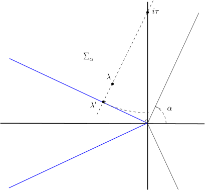
Figure 2. The set $\Sigma_{\alpha}$.

The fact that $T_{A,\varepsilon}(t)$ can be extended to an analytic semigroup $T_{A,\varepsilon}(z)$ on the domain $\Delta_{\alpha}$ is a simple application of (6.15) and Proposition 6.3, with $M:=\frac{1}{1-\sin(\alpha)}$.

Let us then define $\widetilde{T_{A}}(z):=e^{\varepsilon z}T_{A,\varepsilon}(z)$, for $z\in\Delta_{\alpha}$ so that $\widetilde{T_{A}}$ is an analytic extension of $T_{A}$ (an argument of analyticity shows that $\widetilde{T_{A}}$ does not depend on $\varepsilon$). ∎

Remark 6.4.

Note that estimate (6.13) is also valid in the limit as $\varepsilon\to 0$: for all $\alpha\in(0,\frac{\pi}{2})$, $\lambda\in\Sigma_{\alpha}$,

$$\left\|\,R(\lambda,A)\,\right\|_{-1,{q_{0}},\mu}\,\;\leqslant\;\,\frac{1}{1-\sin(\alpha)}\cdot\frac{1}{|\lambda|}\,.$$ (6.16)

Spectral properties of $L^{\omega}_{{q}}=A+B$

In this part, we show that if the perturbation $B$ is small enough with respect to $A$, one has the same spectral properties for $L^{\omega}_{{q}}=A+B$ as for $A$. In this extent, we recall that $\mu$ is of compact support in $[-1,1]$, and the disorder is rescaled by $\delta>0$.

Proposition 6.5.

The operator $B$ is $A$-bounded, in the sense that there exist explicit constants $a_{K,\delta}$ and $b_{K,\delta}$, depending on $K$ and $\delta$ such that for all $u$ in the domain of (the closure of) $A$

$$\left\|\,Bu\,\right\|_{-1,{q_{0}},\mu}\,\;\leqslant\;\,a_{K,\delta}\left\|\,u\,\right\|_{-1,{q_{0}},\mu}+b_{K,\delta}\left\|\,Au\,\right\|_{-1,{q_{0}},\mu}\,.$$ (6.17)

Moreover, for fixed $K>1$, $a_{K,\delta}=O(\delta)$ and $b_{K,\delta}=O(\delta)$, as $\delta\rightarrow 0$.

The latter proposition is based on the fact that the difference $\varepsilon(q)(\theta,\omega,\delta)=q(\theta,\delta\omega)-q_{0}(\theta)$ in (6.7) is small if the scale parameter $\delta$ tend to $0$:

Lemma 6.6.

For $\delta>0$, let us define

$$\left\|\,\varepsilon(q)\,\right\|_{\infty}\,:=\,\sup_{\begin{subarray}{c}\theta\in{\mathbb{S}},|\omega|\;\leqslant\;1\\ 0<u<\delta\end{subarray}}|\varepsilon(q)(\theta,\omega,u)|\,.$$ (6.18)

Then for all $K>1$, $\left\|\,\varepsilon(q)\,\right\|_{\infty}=O(\delta)$, as $\delta\rightarrow 0$. More precisely, for $K>1$, $\delta>0$, the following inequality holds:

$$\left\|\,\varepsilon(q)\,\right\|_{\infty}\,\;\leqslant\;\,\varepsilon_{K,\delta}\,,$$ (6.19)

where the constant $\varepsilon_{K,\delta}$ can be chosen explicitly in terms of $K$ and $\delta$:

$$\varepsilon_{K,\delta}\,:=\,\frac{\delta}{\pi}e^{8\pi\delta}\left(2+3e^{4\pi\delta}\right)e^{14K\bar{r}_{\delta}}\left(1+2\pi e^{2K\bar{r}_{\delta}}\right)\,,$$ (6.20)

where we recall that $\bar{r}_{\delta}=\max\left(r_{0},r_{\delta}\right)$.

Proof of Lemma 6.6.

Recall that the disordered stationary solution $q$ (1.5) is given by

$$q(\theta,\delta\omega)\,:=\,\frac{S(\theta,\delta\omega,2Kr_{\delta})}{Z(\delta\omega,2Kr_{\delta})},$$ (6.21)

where $S(\theta,\omega,x)$ is defined in (1.6) and that the non-disordered one (2.1) is given by $q_{0}(\theta)=\frac{S(\theta,0,2Kr_{0})}{Z(0,2Kr_{0})}=\frac{e^{2Kr_{0}\cos(\theta)}}{\int_{{\mathbb{S}}}e^{2Kr_{0}\cos(\theta)}\,\text{\rm d}\theta}$. Since $q(\theta,\delta\omega)=q(-\theta,-\delta\omega)$, it suffices to consider the case $\delta\omega>0$. A simple computation shows that

$$Z(\delta\omega,2Kr_{\delta})\,\;\geqslant\;\,4\pi^{2}e^{-4Kr_{\delta}}e^{-4\pi\delta}\,,$$ (6.22)

and that

$$|S(\theta,0)|\,\;\leqslant\;\,2\pi e^{4Kr_{0}}\,.$$ (6.23)

Using $|q(\theta,\delta\omega)-q_{0}(\theta)|\;\leqslant\;\frac{1}{Z(\delta\omega)Z(0)}\left(Z(0)|S(\theta,\delta\omega)-S(\theta,0)|+|S(\theta,0)||Z(0)-Z(\delta\omega)|\right)$, one has to deal with, successively:

• for fixed $\theta\in{\mathbb{S}}$, $|S(\theta,\delta\omega)-S(\theta,0)|\;\leqslant\;\delta\cdot\sup_{|\omega|\;\leqslant\;1}|\frac{\,\text{\rm d}}{\,\text{\rm d}\omega}S(\theta,\delta\omega)|$. A long calculation shows that the latter expression $|\frac{\,\text{\rm d}}{\,\text{\rm d}\omega}S(\theta,\delta\omega)|$ can be bounded above by $8\pi^{2}e^{4Kr_{\delta}}e^{4\pi\delta}\left(2+3e^{4\pi\delta}\right)$, that is,

  $$|S(\theta,\delta\omega)-S(\theta,0)|\,\;\leqslant\;\,\delta 8\pi^{2}e^{4Kr_{\delta}}e^{4\pi\delta}\left(2+3e^{4\pi\delta}\right)\,.$$ (6.24)

• Using $|Z(\delta\omega)-Z(0)|=\left|\int_{{\mathbb{S}}}(S(\theta,\delta\omega)-S(\theta,0))\,\text{\rm d}\theta\right|$ and (6.24), one has directly:

  $$|Z(\delta\omega)-Z(0)|\,\;\leqslant\;\,\delta 16\pi^{3}e^{4Kr_{\delta}}e^{4\pi\delta}\left(2+3e^{4\pi\delta}\right)\,.$$ (6.25)

Putting together (6.22), (6.23), (6.24) and (6.25), one obtains the result. ∎

We are now in position to prove the $A$-boundedness of $B$:

Proof of Proposition 6.5.

$B$ is $A$-bounded: let us fix a $u$ in the domain of the closure of $A$. Then we have $\left\|\,Bu\,\right\|_{-1,{q_{0}},\mu}=\left\|\,{\mathcal{B}}u\,\right\|_{2,{q_{0}},\mu}$, where ${\mathcal{B}}u$ is the appropriate primitive of $Bu$, namely:

$${\mathcal{B}}u(\theta,\omega) \,:=\,{}-\left(u(\theta,\omega)\langle J\ast\varepsilon(q)\rangle_{\mu}+\varepsilon(q)(\theta,\omega,\delta)\langle J\ast u\rangle_{\mu}(\theta)+\delta\omega u(\theta,\omega)\right)$$

$$+{}\left(\int_{{\mathbb{S}}}\frac{1}{q_{0}}\right)^{-1}\left(\int_{{\mathbb{S}}}\frac{u(\theta,\omega)\langle J\ast\varepsilon(q)\rangle_{\mu}+\varepsilon(q)(\theta,\omega,\delta)\langle J\ast u\rangle_{\mu}(\theta)+\delta\omega u(\theta,\omega)}{q_{0}(\theta)}\,\text{\rm d}\theta\right)\,.$$ (6.26)

One can easily shows that there exists a constant $c^{(1)}_{K,\delta}$, depending only on $K>1$ and $\delta>0$ such that:

$$\left\|\,Bu\,\right\|_{-1,{q_{0}},\mu}\,\;\leqslant\;\,c^{(1)}_{K,\delta}\left\|\,u\,\right\|_{2,{q_{0}},\mu}\,.$$ (6.27)

Indeed, an easy calculation shows that $|\langle J\ast\varepsilon(q)\rangle_{\mu}|\;\leqslant\;4K\left\|\,\varepsilon(q)\,\right\|_{\infty}$ and that

$$\begin{split}|\langle J\ast u\rangle_{\mu}(\cdot)|&\,\;\leqslant\;\,K\left(\int_{{\mathbb{S}}}\sin(\cdot-\varphi)^{2}q_{0}(\varphi)\,\text{\rm d}\varphi\right)^{\frac{1}{2}}\left\|\,u\,\right\|_{2,{q_{0}},\mu}\\ &\,\;\leqslant\;K\left(\int_{{\mathbb{S}}}q_{0}(\varphi)\,\text{\rm d}\varphi\right)^{\frac{1}{2}}\left\|\,u\,\right\|_{2,{q_{0}},\mu}=K\left\|\,u\,\right\|_{2,{q_{0}},\mu}\,.\end{split}$$ (6.28)

So we have for all $\theta,\omega$ (recall that $Z_{0}$ is the normalization constant in (2.1)):

$$\begin{split}|{\mathcal{B}}u(\theta,\omega)|\,\;\leqslant\;\,&\left(4K\left\|\,\varepsilon(q)\,\right\|_{\infty}+\delta|\omega|\right)|u|+2K\left\|\,\varepsilon(q)\,\right\|_{\infty}\left\|\,u\,\right\|_{2,{q_{0}},\mu}\\ &+Z_{0}^{-1}\left(4K\left\|\,\varepsilon(q)\,\right\|_{\infty}+\delta|\omega|\right)\left(\int_{{\mathbb{S}}}\frac{|u|^{2}}{q_{0}}\right)^{\frac{1}{2}}\,.\end{split}$$ (6.29)

Hence, inequality (6.27) is true for the following choice of $c^{(1)}_{K,\delta}$ (recall that $\varepsilon_{K,\delta}$ is defined in (6.20)):

$$c^{(1)}_{K,\delta}\,:=\,\left(6\left(4K\varepsilon_{K,\delta}+\delta\right)^{2}+12K^{2}Z_{0}^{2}\varepsilon_{K,\delta}^{2}\right)^{\frac{1}{2}}\,.$$ (6.30)

Remark 6.7.

Note that, thanks to Lemma 6.6, one has that $c^{(1)}_{K,\delta}=O(\delta)$ as $\delta\rightarrow 0$.

In order to complete the proof of the inequality (6.17), it suffices to prove that there exist constants $c^{(2)}_{K}$ and $c^{(3)}_{K}$, only depending on $K$ such that, for all $u$:

$$\left\|\,u\,\right\|_{2,{q_{0}},\mu}\,\;\leqslant\;\,c^{(2)}_{K}\left\|\,Au\,\right\|_{-1,{q_{0}},\mu}+c^{(3)}_{K}\left\|\,u\,\right\|_{-1,{q_{0}},\mu}\,.$$ (6.31)

The rest of this first of the proof is devoted to find explicit expressions of $c^{(2)}_{K}$ and $c^{(3)}_{K}$, and is based on an interpolation argument.

For all integer $n>1$, one can compute the linear operator $f\mapsto f^{\prime}$ in terms of a sum of two integral operators, namely:

$$f^{\prime}\,=\,I_{n}(f^{\prime\prime})+J_{n}(f)\,,$$ (6.32)

where $I_{n}:f\mapsto\int_{0}^{2\pi}i_{n}(\theta,\varphi)f(\varphi)\,\text{\rm d}\varphi$ (resp. $J_{n}:f\mapsto\int_{0}^{2\pi}j_{n}(\theta,\varphi)f(\varphi)\,\text{\rm d}\varphi$) is the integral operator whose kernel $i_{n}(\theta,\varphi)$ (resp. $j_{n}(\theta,\varphi)$) is defined by:

$$\left\{\begin{array}[]{lll}i_{n}(\theta,\varphi)\,:=\,\frac{\varphi^{n+1}}{2\pi\theta^{n}}\,,&j_{n}(\theta,\varphi)\,:=\,-\frac{n(n+1)\varphi^{n-1}}{2\pi\theta^{n}}\,,&0\,\;\leqslant\;\,\varphi\,<\,\theta\,\;\leqslant\;\,2\pi\,,\\[10.0pt] i_{n}(\theta,\varphi)\,:=\,\frac{-(2\pi-\varphi)^{n+1}}{2\pi(2\pi-\theta)^{n}}\ ,&j_{n}(\theta,\varphi)\,:=\,\frac{n(n+1)(2\pi-\varphi)^{n-1}}{2\pi(2\pi-\theta)^{n}}\ ,&0\,\;\leqslant\;\,\theta\,<\,\varphi\,\;\leqslant\;\,2\pi\,.\end{array}\right.$$ (6.33)

Equality (6.32) can be easily verified by integrations by parts. Since,

$$\left\{\begin{array}[]{ll}\int_{0}^{2\pi}\left|i_{n}(\theta,\varphi)\right|\,\text{\rm d}\varphi\,\;\leqslant\;\,\frac{2\pi}{n+2},&\int_{0}^{2\pi}\left|i_{n}(\theta,\varphi)\right|\,\text{\rm d}\theta\,\;\leqslant\;\,\frac{2\pi}{n-1}\,,\\[10.0pt] \int_{0}^{2\pi}\left|j_{n}(\theta,\varphi)\right|\,\text{\rm d}\varphi\,\;\leqslant\;\,\frac{n+1}{\pi}\,,&\int_{0}^{2\pi}\left|j_{n}(\theta,\varphi)\right|\,\text{\rm d}\theta\,\;\leqslant\;\,\frac{n(n+1)}{\pi(n-1)}\,,\end{array}\right.$$ (6.34)

we see (cf. [12, p.143-144]) that $I_{n}$ and $J_{n}$ are bounded operators on $L^{2}({{\mathbb{S}}})$, namely:

$$\|{I_{n}}\|\,\;\leqslant\;\,\frac{2\pi}{n-1},\quad\|{J_{n}}\|\,\;\leqslant\;\,\frac{n(n+1)}{\pi(n-1)}\,.$$ (6.35)

So, applying relation (6.32) for $f={\mathcal{U}}$ we get, for $\mu$-almost every $\omega$:

$$\left(\int_{{\mathbb{S}}}|u(\theta,\omega)|^{2}\,\text{\rm d}\theta\right)^{\frac{1}{2}}\;\leqslant\;\frac{2\pi}{n-1}\left(\int_{{\mathbb{S}}}|u^{\prime}(\theta,\omega)|^{2}\,\text{\rm d}\theta\right)^{\frac{1}{2}}+\frac{n(n+1)}{\pi(n-1)}\left(\int_{{\mathbb{S}}}|{\mathcal{U}}(\theta,\omega)|^{2}\,\text{\rm d}\theta\right)^{\frac{1}{2}}.$$ (6.36)

This gives

$$\left\|\,u\,\right\|_{2,\mu}\,\;\leqslant\;\,\frac{2\pi}{n-1}\left\|\,u^{\prime}\,\right\|_{2,\mu}+\frac{n(n+1)}{\pi(n-1)}\left\|\,{\mathcal{U}}\,\right\|_{2,\mu}\,.$$ (6.37)

Since $\left\|\,{\mathcal{U}}\,\right\|_{2,{q_{0}},\mu}=\left\|\,u\,\right\|_{-1,{q_{0}},\mu}$, it only remains to control $\left\|\,u^{\prime}\,\right\|_{2,{q_{0}},\mu}$ with $\left\|\,Au\,\right\|_{-1,{q_{0}},\mu}$: like for the beginning of this proof for the operator $B$, we have $\left\|\,Au\,\right\|_{-1,{q_{0}},\mu}=\left\|\,{\mathcal{A}}u\,\right\|_{2,{q_{0}},\mu}$, where ${\mathcal{A}}u$ is the appropriate primitive of $Au$:

$${\mathcal{A}}u(\theta,\omega) \,:=\,{}{\frac{1}{2}}u^{\prime}(\theta,\omega)-\left(u(\theta,\omega)(J\ast q_{0})+q_{0}(\theta)\langle J\ast u\rangle_{\mu}(\theta)\right)$$

$$+{}\left(\int_{{\mathbb{S}}}\frac{1}{q_{0}}\right)^{-1}\left(\int_{{\mathbb{S}}}\left\{\frac{u(\theta,\omega)(J\ast q_{0})}{q_{0}(\theta)}+{\frac{1}{2}}u(\theta,\omega)\partial_{\theta}\left(\frac{1}{q_{0}(\theta)}\right)\right\}\,\text{\rm d}\theta\right)\,.$$ (6.38)

Using inequalities $|\langle J\ast u\rangle|_{\mu}(\cdot)\;\leqslant\;K\sqrt{\pi}\left\|\,u\,\right\|_{2,\mu}$, and $\int_{{\mathbb{S}}}\frac{|u(\cdot,\omega)|}{q_{0}}\;\leqslant\;Z_{0}^{\frac{1}{2}}e^{Kr_{0}}\left(\int_{{\mathbb{S}}}|u(\cdot,\omega)^{2}|\right)^{\frac{1}{2}}$, an easy calculation shows that:

$$|u^{\prime}(\cdot,\omega)|\,\;\leqslant\;\,2|{\mathcal{A}}u(\cdot,\omega)|+2Kr_{0}|u(\cdot,\omega)|+2\sqrt{\pi}Kq_{0}(\cdot)\left\|\,u\,\right\|_{2,\mu}+\frac{4Kr_{0}}{Z_{0}^{\frac{1}{2}}}e^{Kr_{0}}\left(\int_{{\mathbb{S}}}|u(\cdot,\omega)^{2}|\right)^{\frac{1}{2}}\,,$$ (6.39)

and thus,

$$\left\|\,u^{\prime}\,\right\|_{2,\mu}\,\;\leqslant\;\,4\left\|\,{\mathcal{A}}u\,\right\|_{2,\mu}+4K\left(r_{0}^{2}+\pi Z_{0}^{-1}e^{2Kr_{0}}(1+8r_{0}^{2})\right)^{\frac{1}{2}}\left\|\,u\,\right\|_{2,\mu}\,,$$ (6.40)

and by putting (6.37) and (6.40) together we obtain

$$\begin{split}\left\|\,u\,\right\|_{2,\mu}\,\;\leqslant\;\,&\frac{8\pi}{n-1}\left\|\,{\mathcal{A}}u\,\right\|_{2,\mu}+\frac{2\pi}{n-1}4K\left(r_{0}^{2}+\pi Z_{0}^{-1}e^{2Kr_{0}}(1+8r_{0}^{2})\right)^{\frac{1}{2}}\left\|\,u\,\right\|_{2,\mu}\\ &+\frac{n(n+1)}{\pi(n-1)}\left\|\,u\,\right\|_{-1,{q_{0}},\mu}\,.\end{split}$$ (6.41)

Let us choose the integer $n=\left\lfloor 16\pi K\left(r_{0}^{2}+\pi Z_{0}^{-1}e^{2Kr_{0}}(1+8r_{0}^{2})\right)^{\frac{1}{2}}+1\right\rfloor$ so that

$$\frac{2\pi}{n-1}4K\left(r_{0}^{2}+\pi Z_{0}^{-1}e^{2Kr_{0}}(1+8r_{0}^{2})\right)^{\frac{1}{2}}\,\;\leqslant\;\,{\frac{1}{2}}\,.$$ (6.42)

In this case, we obtain:

$$\left\|\,u\,\right\|_{2,{q_{0}},\mu} \,\;\leqslant\;\,\frac{e^{2Kr_{0}}}{4K\left(r_{0}^{2}+\pi Z_{0}^{-1}e^{2Kr_{0}}(1+8r_{0}^{2})\right)^{\frac{1}{2}}}\left\|\,Au\,\right\|_{-1,{q_{0}},\mu}$$

$$+\frac{e^{2Kr_{0}}\left(16K\left(r_{0}^{2}+\pi Z_{0}^{-1}e^{2Kr_{0}}(1+8r_{0}^{2})\right)^{\frac{1}{2}}+3\right)^{2}}{16\pi^{2}K\left(r_{0}^{2}+\pi Z_{0}^{-1}e^{2Kr_{0}}(1+8r_{0}^{2})\right)^{\frac{1}{2}}}\left\|\,u\,\right\|_{-1,{q_{0}},\mu}\,,$$ (6.43)

which is precisely the inequality (6.31) we wanted to prove. Inequalities (6.27) and (6.31) give the result, for $a_{K,\delta}:=c^{(1)}_{K,\delta}\cdot c_{K}^{(3)}$ and $b_{K,\delta}:=c^{(1)}_{K,\delta}\cdot c_{K}^{(2)}$.∎

Proposition 6.8.

For all $K>1$, there exists $\delta_{3}(K)>0$ such that for all $0<\delta\;\leqslant\;\delta_{3}(K)$, the operator $L^{\omega}_{{q}}$ is closable. In that case, its closure has the same domain as the closure of $A$.

Proof.

Let us choose $\delta_{3}(K)>0$ so that

$$b_{K,\delta_{3}(K)}<1$$ (6.44)

where $b_{K,\delta}$ is the constant introduced in (6.17), then, for all $0<\delta\;\leqslant\;\delta_{3}(K)$, the operator $B$ is $A$-bounded with $A$-bound strictly lower than $1$. The result is then a consequence of Th. IV-1.1, p.190 in [12]. ∎

The spectrum of $L^{\omega}_{{q}}$

We divide our study into two parts: the determination of the position of the spectrum within a sector and its position near $0$.

Position of the spectrum away from $0$

We prove mainly that the perturbed operator $L^{\omega}_{{q}}$ still generates an analytic semigroup of operators on an appropriate sector. An immediate corollary is the fact that the spectrum lies in a cone whose vertex is zero.

We know (Proposition 6.2) that for all $0<\alpha<\frac{\pi}{2}$, $A$ generates an analytic semigroup of operators on $\Delta_{\alpha}:=\left\{\lambda\in{\mathbf{C}}\,;\,|\arg(\lambda)|<\alpha\right\}$.

Proposition 6.9.

For all $K>1$, $0<\alpha<\frac{\pi}{2}$ and $\varepsilon>0$, there exists $\delta_{4}>0$ (depending on $\alpha$, $K$ and $\varepsilon$) such that for all $0<\delta<\delta_{4}$, the spectrum of $L^{\omega}_{{q}}=A+B$ lies within $\Theta_{\varepsilon,\alpha}:=\left\{\lambda\in{\mathbf{C}}\,;\,\frac{\pi}{2}+\alpha\;\leqslant\;\arg(\lambda)\;\leqslant\;\frac{3\pi}{2}-\alpha\right\}\cup\left\{\lambda\in{\mathbf{C}}\,;\,|\lambda|\;\leqslant\;\varepsilon\right\}$. Moreover, there exists $\alpha^{\prime}\in(0,\frac{\pi}{2})$ such that the operator $L^{\omega}_{{q}}$ still generates an analytic semigroup on $\Delta_{\alpha^{\prime}}$.

Proof of Proposition 6.9.

Let $0<\alpha<\frac{\pi}{2}$ be fixed. Following (6.17) and using (6.16), one can easily deduce an estimate on the bounded operator $BR(\lambda,A)$, for $\lambda\in\Sigma_{\alpha}$:

$$\begin{split}\left\|\,BR(\lambda,A)u\,\right\|_{-1,{q_{0}},\mu}&\,\;\leqslant\;\,a_{K,\delta}\left\|\,R(\lambda,A)u\,\right\|_{-1,{q_{0}},\mu}+b_{K,\delta}\left\|\,AR(\lambda,A)u\,\right\|_{-1,{q_{0}},\mu}\\ &\,\;\leqslant\;\,a_{K,\delta}\frac{1}{(1-\sin(\alpha))|\lambda|}\left\|\,u\,\right\|_{-1,{q_{0}},\mu}\\ &\ \ \ \ \ \ +b_{K,\delta}\left(1+\frac{1}{1-\sin(\alpha)}\right)\left\|\,u\,\right\|_{-1,{q_{0}},\mu}\,.\end{split}$$ (6.45)

Let us fix $\varepsilon>0$ and choose $\delta$ so that:

$$\max\left(4b_{K,\delta}\left(\frac{1}{1-\sin(\alpha)}+1\right),\frac{4a_{K,\delta}}{(1-\sin(\alpha))\varepsilon}\right)\,\;\leqslant\;\,1\,.$$ (6.46)

Then, for $\lambda\in\Sigma_{\alpha}$ such that $|\lambda|>\varepsilon\;\geqslant\;\frac{4a_{K,\delta}}{1-\sin(\alpha)}$, we have

$$\left\|\,BR(\lambda,A)u\,\right\|_{-1,{q_{0}},\mu}\,\;\leqslant\;\,\frac{1}{2}\left\|\,u\,\right\|_{-1,{q_{0}},\mu}\,.$$ (6.47)

In particular, $1-BR(\lambda,A)$ is invertible with $\left\|\,\left(1-BR(\lambda,A)\right)^{-1}\,\right\|_{-1,{q_{0}},\mu}\;\leqslant\;2$. A direct calculation shows that

$$\left(\lambda-(A+B)\right)^{-1}\,=\,R(\lambda,A)\left(1-BR(\lambda,A)\right)^{-1}\,.$$ (6.48)

One deduces the following estimates on the resolvent: for $\lambda\in\Sigma_{\alpha}$, $|\lambda|>\varepsilon$,

$$\left\|\,R(\lambda,L^{\omega}_{{q}})\,\right\|_{-1,{q_{0}},\mu}\,\;\leqslant\;\,\frac{2}{(1-\sin(\alpha))|\lambda|}\,.$$ (6.49)

Estimate (6.49) has two consequences: firstly, one deduces immediately that the spectrum $\sigma(L^{\omega}_{q})$ of $L^{\omega}_{q}$ is contained in $\Theta_{\varepsilon,\alpha}$:

$$\sigma(L_{q}^{\omega})\subseteq\left\{\lambda\in{\mathbf{C}}\,;\,\frac{\pi}{2}+\alpha\;\leqslant\;\arg(\lambda)\;\leqslant\;\frac{3\pi}{2}-\alpha\right\}\cup\left\{\lambda\in{\mathbf{C}}\,;\,|\lambda|\;\leqslant\;\varepsilon\right\}.$$ (6.50)

Secondly, (6.49) entails that $L^{\omega}_{q}$ generates an analytic semigroup of operators on an appropriate sector. Indeed, if one denotes by $L^{\omega}_{q,\varepsilon}:=L^{\omega}_{q}-\varepsilon$, one deduces from (6.50) that $0\in\rho(L^{\omega}_{q,2\varepsilon})$ and that for all $\lambda\in{\mathbf{C}}$ with $\Re(\lambda)>0$ (in particular, $|\lambda|<|\lambda+2\varepsilon|$)

$$\left\|\,R(\lambda,L^{\omega}_{{q,2\varepsilon}})\,\right\|_{-1,{q_{0}},\mu}\, =\,\left\|\,R(\lambda+2\varepsilon,L^{\omega}_{{q}})\,\right\|_{-1,{q_{0}},\mu}\,\;\leqslant\;\,\frac{2}{(1-\sin(\alpha))|\lambda+2\varepsilon|}\,,$$

$$\,\;\leqslant\;\,\frac{2}{(1-\sin(\alpha))|\lambda|}\,.$$ (6.51)

Hence, using the same arguments of Taylor expansion as in the proof of Proposition 6.2 and applying Proposition 6.3, one easily sees that $L^{\omega}_{{q,2\varepsilon}}$ generates an analytic semigroup in a (a priori) smaller sector $\Delta_{\alpha^{\prime}}$, where $\alpha^{\prime}\in(0,\frac{\pi}{2})$ can be chosen as $\alpha^{\prime}:=\frac{1}{2}\arctan\left(\frac{1-\sin(\alpha)}{2}\right)$. But if $L^{\omega}_{{q,2\varepsilon}}$ generates an analytic semigroup, so does $L^{\omega}_{q}$. ∎

Position of the spectrum near $0$

Let us apply Proposition 6.9 for fixed $K>1$, $\alpha\in(0,\frac{\pi}{2})$, $\rho\in(0,1)$ and $\varepsilon:=\rho\lambda_{K}$, where we recall that $\lambda_{K}$ is the spectral gap between the eigenvalue $0$ for the non perturbed operator $A$ and the rest of the spectrum $\sigma(A)\smallsetminus\{0\}$. Let $\Theta_{\varepsilon,\alpha}^{+}:=\left\{\lambda\in\Theta_{\varepsilon,\alpha}\,;\,\Re(\lambda)\;\geqslant\;0\right\}$ be the subset of $\Theta_{\varepsilon,\alpha}$ which lies in the positive part of the complex plane (see Fig. 3). In order to show the linear stability, one has to make sure that one can choose a perturbation $B$ small enough so that no eigenvalue of $A+B$ remains in the small set $\Theta_{\varepsilon,\alpha}^{+}$.

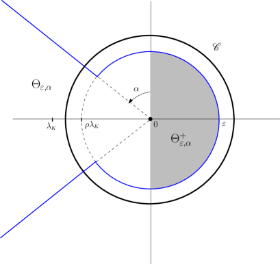
Figure 3. The set $\Theta_{\varepsilon,\alpha}$.

Since $\lambda_{K}>0$, one can separate $0$ from the rest of the spectrum of $A$ by a circle $\mathscr{C}$ centered in $0$ with radius $(\frac{\rho+1}{2})\lambda_{K}$. The appropriate choice of $\varepsilon$ ensures that the interior of the disk delimited by $\mathscr{C}$ contains $\Theta_{\varepsilon,\alpha}^{+}$ (see Figure 3).

The main argument is the following: by construction of $\mathscr{C}$, $0$ is the only eigenvalue (with multiplicity $1$) of the non-perturbed operator $A$ lying in the interior of $\mathscr{C}$. A principle of local continuity of eigenvalues shows that, while adding a sufficiently small perturbation $B$ to $A$, the interior of $\mathscr{C}$ still contains exactly one eigenvalue (which is a priori close but not equal to $0$) with the same multiplicity.

But we already know that for the perturbed operator $L^{\omega}_{{q}}=A+B$, $0$ is always an eigenvalue (since $L^{\omega}_{{q}}q^{\prime}=0$). One can therefore conclude that, by uniqueness, $0$ is the only element of the spectrum of $L^{\omega}_{{q}}$ within $\mathscr{C}$, and is an eigenvalue with multiplicity $1$. In particular, there is no element of the spectrum in the positive part of the complex plane.

In order to quantify the appropriate size of the perturbation $B$, one has to have explicit estimates on the resolvent $R(\lambda,A)$ on the circle $\mathscr{C}$.

Lemma 6.10.

There exists some explicit constant $c_{\mathscr{C}}=c_{\mathscr{C}}(K,\rho)$ such that for all $\lambda\in\mathscr{C}$,

$$\left\|\,R(\lambda,A)\,\right\|_{-1,{q_{0}},\mu} \,\;\leqslant\;\,c_{\mathscr{C}}\,,$$ (6.52)

$$\left\|\,AR(\lambda,A)\,\right\|_{-1,{q_{0}},\mu} \,\;\leqslant\;\,1+\left(\frac{1+\rho}{2}\right)\lambda_{K}\cdot c_{\mathscr{C}}\,.$$ (6.53)

One can choose $c_{\mathscr{C}}$ as $\frac{1}{\lambda_{K}}\max\left(\frac{2}{\rho+1},\,\frac{2}{1-\rho}\right):=\frac{\ell(\rho)}{\lambda_{K}}$.

Proof of Lemma 6.10.

Applying the spectral theorem (see [23, Th. 3, p.1192]) to the essentially self-adjoint operator $A$, there exists a spectral measure $E$ vanishing on the complementary of the spectrum of $A$ such that $A=\int_{{\mathbb{R}}}\lambda\,\text{\rm d}E(\lambda)$. In that extent, one has for any $\zeta\in\mathscr{C}$

$$R(\zeta,A)\,=\,\int_{{\mathbb{R}}}\frac{\,\text{\rm d}E(\lambda)}{\lambda-\zeta}\,.$$ (6.54)

In particular, for $\zeta\in\mathscr{C}$

$$\left\|\,R(\zeta,A)\,\right\|_{-1,{q_{0}},\mu}\;\leqslant\;\sup_{\lambda\in\sigma(A)}\frac{1}{|\lambda-\zeta|}\;\leqslant\;\frac{\ell(\rho)}{\lambda_{K}}\,.$$ (6.55)

The estimation (6.53) is straightforward. ∎

We are now in position to apply our argument of local continuity of eigenvalues: Following [12, Th III-6.17, p.178], there exists a decomposition of the operator $A$ according to $H^{-1}_{{q_{0}},\mu}=H_{0}\oplus H^{\prime}$ (in the sense that $AH_{0}\subset H_{0}$, $AH^{\prime}\subset H^{\prime}$ and $P{\mathcal{D}}(A)\subset{\mathcal{D}}(A)$, where $P$ is the projection on $H_{0}$ along $H^{\prime}$) in such a way that $A$ restricted to $H_{0}$ has spectrum $\{0\}$ and $A$ restricted to $H^{\prime}$ has spectrum $\sigma(A)\smallsetminus\{0\}$.

Let us note that the dimension of $H_{0}$ is $1$, since the characteristic space of $A$ in the eigenvalue $0$ is reduced to its kernel which is of dimension $1$.

Then, applying [12, Th. IV-3.18, p.214], and using Proposition 6.5, we find that if one chooses $\delta>0$, such that

$$\sup_{\lambda\in\mathscr{C}}\left(a_{K,\delta}\left\|\,R(\lambda,A)\,\right\|_{-1,{q_{0}},\mu}+b_{K,\delta}\left\|\,AR(\lambda,A)\,\right\|_{-1,{q_{0}},\mu}\right)<1,$$ (6.56)

then the perturbed operator $L^{\omega}_{{q}}$ is likewise decomposed according to $H^{-1}_{{q_{0}},\mu}=\widetilde{H}_{0}\oplus\widetilde{H}^{\prime}$, in such a way that $\dim(H_{0})=\dim(\widetilde{H}_{0})=1$, and that the spectrum of $L^{\omega}_{{q}}$ is again separated in two parts by $\mathscr{C}$ . But we already know that the characteristic space of the perturbed operator $L^{\omega}_{{q}}$ according to the eigenvalue $0$ is, at least, of dimension $1$ (since $L^{\omega}_{{q}}q^{\prime}=0$).

We can conclude, that for such an $\delta>0$, $0$ is the only eigenvalue in $\mathscr{C}$ and that $\dim(\widetilde{H}_{0})=1$.

Applying Lemma 6.10, we see that condition (6.56) is satisfied if we choose $\delta>0$ so that:

$$a_{K,\delta}c_{\mathscr{C}}+b_{K,\delta}\left(1+\left(\frac{1+\rho}{2}\right)\lambda_{K}c_{\mathscr{C}}\right)<1.$$ (6.57)

In particular, in that case, the spectrum of $L^{\omega}_{{q}}$ is contained in

$$\left\{\lambda\in{\mathbb{C}}\,;\,\frac{\pi}{2}+\alpha\;\leqslant\;\arg(\lambda)\;\leqslant\;\frac{3\pi}{2}-\alpha\right\}\subseteq\left\{z\in{\mathbf{C}}\,;\,\Re(z)\;\leqslant\;0\right\}\,.$$ (6.58)

Finally, the following proposition sums-up the sufficient conditions on $\delta$ for the conclusions of Theorem 2.5 to be satisfied:

Proposition 6.11.

Recall the definitions of $a_{K,\delta}$ and $b_{K,\delta}$ in Proposition 6.5. If $\delta>0$ satisfies the following conditions

$$\begin{split}b_{K,\delta}&\,\;\leqslant\;\,1\,,\\ 4b_{K,\delta}\left(\frac{1}{1-\sin(\alpha)}+1\right)&\,\;\leqslant\;\,1\,,\\ \frac{4a_{K,\delta}}{\rho\lambda_{K}\left(1-\sin(\alpha)\right)}&\,\;\leqslant\;\,1\,,\\ a_{K,\delta}\frac{\ell(\rho)}{\lambda_{K}}+b_{K,\delta}\left(1+\left(\frac{1+\rho}{2}\right)\ell(\rho)\right)&\,<\,1\,.\end{split}$$ (6.59)

the conclusions of Theorem 2.5 are true.

Proof.

One has simply to sum-up conditions (6.44), (6.46) with $\varepsilon=\rho\lambda_{K}$ and (6.57). (6.60) can be obtained by (long) estimations on the coefficients $a_{K,\delta}$ and $b_{K,\delta}$. ∎

Remark 6.12.

The conditions in Proposition 6.11 can be simplified. For example one can exhibit an explicit constant $c$ such that if $\delta$ satisfies

$$\begin{split}\delta e^{12\pi\delta}\,\;\leqslant\;\,ce^{-20K\bar{r_{\delta}}}\max&\left(1,\left(\frac{1-\sin(\alpha)}{2-\sin(\alpha)}\right),\frac{\rho\lambda_{K}(1-\sin(\alpha))e^{-4K\bar{r_{\delta}}}}{K^{2}},\right.\\ &\left.\ \ \ \ \frac{\lambda_{K}}{K^{2}e^{4K\bar{r_{\delta}}}\ell(\rho)+\lambda_{K}\left(1+\left(\frac{1+\rho}{2}\right)\ell(\rho)\right)}\right)\end{split}$$ (6.60)

the conditions in (6.59) are fulfilled. Explicit estimates on the spectral gap $\lambda_{K}$ can be found in [3, Sec. 2.5].

Appendix A Regularity in the non-linear Fokker-Planck equation

The purpose of this section is to establish regularity properties of the solution of the non-linear equation (1.13) (where we fix $\delta=1$ for simplicity). Note that this case also captures the situation where $U(\cdot,\omega)\equiv\omega$ (evolution (1.4)), as well as the situation where $U(\cdot,\cdot)\equiv 0$ (evolution (1.12)). In what follows we make the assumption that $U$ is bounded and that for all $\omega\in\operatorname*{Supp}(\mu)$, $\theta\mapsto U(\theta,\omega)\in C^{\infty}({\mathbb{S}};\,{\mathbb{R}})$ with bounded derivatives.

The existence and uniqueness in $L^{2}(\lambda\otimes\omega)$ of a solution to (1.13) can be tackled using Banach fixed point arguments (see [18, Section 4.7]), but one can obtain more regularity from the theory of fundamental solutions of parabolic equations.

More precisely, it is usual to interpret Equation (1.13) as the strong formulation of the weak equation (where $\nu\in{\mathcal{C}}([0,T],{\mathcal{M}}_{1}({\mathbb{S}}\times{\mathbb{R}}))$ and $F$ is any bounded function on ${\mathbb{S}}\times{\mathbb{R}}$ with twice bounded derivatives w.r.t. $\theta$):

$$\int_{{\mathbb{R}}\times{{\mathbb{S}}}}F(\theta,\omega)\nu_{t}(\,\text{\rm d}\theta,\,\text{\rm d}\omega) =\int_{{\mathbb{R}}\times{{\mathbb{S}}}}F(\theta,\omega)\nu_{0}(\,\text{\rm d}\theta,\,\text{\rm d}\omega)+\frac{1}{2}\int_{0}^{t}\int_{{\mathbb{R}}\times{{\mathbb{S}}}}F^{\prime\prime}(\theta,\omega)\nu_{s}(\,\text{\rm d}\theta,\,\text{\rm d}\omega)\,\text{\rm d}s$$

$$+\int_{0}^{t}\int_{{\mathbb{R}}\times{{\mathbb{S}}}}F^{\prime}(\theta,\omega)\left(\int_{{\mathbb{R}}\times{{\mathbb{S}}}}J(\theta-\cdot)\,\text{\rm d}\nu_{s}+U(\theta,\omega)\right)\nu_{s}(\,\text{\rm d}\theta,\,\text{\rm d}\omega)\,\text{\rm d}s,$$ (A.1)

where the second marginal (w.r.t. to the disorder $\omega$) of the initial condition $\nu_{0}(\,\text{\rm d}\theta,\,\text{\rm d}\omega)$ is $\mu(\,\text{\rm d}\omega)$ so that one can write

$$\nu_{0}(\,\text{\rm d}\theta,\,\text{\rm d}\omega)=\nu_{0}^{\omega}(\,\text{\rm d}\theta)\mu(\,\text{\rm d}\omega)\,,$$ (A.2)

where $\nu_{0}^{\omega}$ is a probability measure on ${\mathbb{S}}$, for $\mu$-a.e. $\omega$.

As already mentioned, a proof of the existence of a solution on $[0,T]$ of (A.1) can be obtained from the almost-sure convergence of the empirical measure of the microscopic system [13]. One can also find a proof of uniqueness of such a solution relying on arguments introduced in [14].

The regularity result can be stated as follows:

Proposition A.1.

For all probability measure $\nu_{0}(\,\text{\rm d}\theta,\,\text{\rm d}\omega)=\nu_{0}^{\omega}(\,\text{\rm d}\theta)\mu(\,\text{\rm d}\omega)$ on ${\mathbb{S}}\times{\mathbb{R}}$, for all $T>0$, there exists a unique solution $\nu$ to (A.1) in ${\mathcal{C}}([0,T],{\mathcal{M}}_{1}({\mathbb{S}}\times{\mathbb{R}}))$ such that for all $F\in{\mathcal{C}}({\mathbb{S}}\times{\mathbb{R}})$,

$$\lim_{t\searrow 0}\int_{{\mathbb{R}}\times{{\mathbb{S}}}}F(\theta,\omega)\nu_{t}(\,\text{\rm d}\theta,\,\text{\rm d}\omega)=\int_{{\mathbb{R}}\times{{\mathbb{S}}}}F(\theta,\omega)\nu_{0}^{\omega}(\,\text{\rm d}\theta)\mu(\,\text{\rm d}\omega).$$ (A.3)

Moreover, for all $t>0$, $\nu_{t}$ is absolutely continuous with respect to $\lambda_{1}\otimes\mu$ and for $\mu$-a.e. $\omega\in Supp(\mu)$, its density $(t,\theta,\omega)\mapsto p_{t}(\theta,\omega)$ is strictly positive on $(0,T]\times{\mathbb{S}}$, is ${\mathcal{C}}^{\infty}$ in $(t,\theta)$ and solves the Fokker-Planck equation (1.13).

Proof of Proposition A.1.

Let us fix $T>0$, $\omega\in\operatorname*{Supp}(\mu)$ and $t\mapsto\nu_{t}$ the unique solution in ${\mathcal{C}}([0,T],{\mathcal{M}}_{1}({\mathbb{S}}\times{\mathbb{R}}))$ to (A.1). Let us define $R(t,\theta,\omega):=\int_{{\mathbb{R}}\times{{\mathbb{S}}}}J(\theta-\cdot)\,\text{\rm d}\nu_{t}+U(\theta,\omega)$ and consider the linear equation

$$\partial_{t}p_{t}(\theta,\omega)\,=\,\frac{1}{2}\Delta p_{t}(\theta,\omega)-\partial_{\theta}\Big{(}p_{t}(\theta,\omega)R(t,\theta,\omega)\Big{)}\,,$$ (A.4)

such that for $\mu$-a.e. $\omega$, for all $F\in{\mathcal{C}}({\mathbb{S}})$,

$$\int_{{\mathbb{S}}}F(\theta)p_{t}(\theta,\omega)\,\text{\rm d}\theta\,\stackrel{{\scriptstyle t\searrow 0}}{{\longrightarrow}}\int_{{\mathbb{S}}}F(\theta)\nu_{0}^{\omega}(\,\text{\rm d}\theta)\,.$$ (A.5)

For fixed $\omega\in\operatorname*{Supp}(\mu)$, $R(\cdot,\cdot,\omega)$ is continuous in time and ${\mathcal{C}}^{\infty}$ in $\theta$.

Suppose for a moment that we have found a weak solution $p_{t}(\theta,\omega)$ to (A.4)-(A.5) such that for $\mu$-a.e. $\omega$, $p_{t}(\cdot,\omega)$ is strictly positive on $(0,T]\times{\mathbb{S}}$. In particular for such a solution $p$, the quantity $\int_{{\mathbb{S}}}p_{t}(\theta,\omega)\,\text{\rm d}\theta$ is conserved for $t>0$, so that $p_{t}(\cdot,\omega)$ is indeed a probability density for all $t>0$. Then both probability measures $\nu_{t}(\,\text{\rm d}\theta,\,\text{\rm d}\omega)$ and $p_{t}(\theta,\omega)\,\text{\rm d}\theta\mu(\,\text{\rm d}\omega)$ solve

$$\int_{{\mathbb{R}}\times{{\mathbb{S}}}}F(\theta,\omega)\nu_{t}(\,\text{\rm d}\theta,\,\text{\rm d}\omega) =\int_{{\mathbb{R}}\times{{\mathbb{S}}}}F(\theta,\omega)\nu_{0}(\,\text{\rm d}\theta,\,\text{\rm d}\omega)+\frac{1}{2}\int_{0}^{t}\int_{{\mathbb{R}}\times{{\mathbb{S}}}}F^{\prime\prime}(\theta,\omega)\nu_{s}(\,\text{\rm d}\theta,\,\text{\rm d}\omega)\,\text{\rm d}s$$

$$+\int_{0}^{t}\int_{{\mathbb{R}}\times{{\mathbb{S}}}}F^{\prime}(\theta,\omega)R(t,\theta,\omega)\nu_{s}(\,\text{\rm d}\theta,\,\text{\rm d}\omega)\,\text{\rm d}s.$$ (A.6)

By [13] or [14, Lemma 10], uniqueness in (A.1) is precisely a consequence of uniqueness in (A.6). Hence, by uniqueness in (A.6), $\nu_{t}(\,\text{\rm d}\theta,\,\text{\rm d}\omega)=p_{t}(\theta,\omega)\,\text{\rm d}\theta\mu(\,\text{\rm d}\omega)$, which is the result. So it suffices to exhibit a weak solution $p_{t}(\theta,\omega)$ to (A.4) such that (A.5) is satisfied.

This fact can be deduced from standard results for uniform parabolic PDEs (see [2] and [6] for precise definitions). In particular, a usual result, which can be found in [2, §7 p.658], states that (A.4) admits a fundamental solution $\Gamma(\theta,t;\theta^{\prime},s,\omega)$ ($t>s$), which is bounded above and below (see [2, Th.7, p.661]):

$$\frac{1}{C\sqrt{t-s}}\exp\left(\frac{-C(\theta-\theta^{\prime})^{2}}{\sqrt{t-s}}\right)\;\leqslant\;\Gamma(\theta,t;\theta^{\prime},s,\omega)\;\leqslant\;\frac{C}{\sqrt{t-s}}\exp\left(\frac{-(\theta-\theta^{\prime})^{2}}{C\sqrt{t-s}}\right)\,.$$ (A.7)

Note that the constant $C>0$ only depends on $T$ and the structure of the linear operator in (A.4) (see [2, Th.7, p.661] and [2, §1, p.615]). In particular, since $(\theta,\omega)\mapsto U(\theta,\omega)$ is bounded, this constant does not depend on $\omega$.

Note that the proof given in [2] is done for $\theta\in{\mathbb{R}}$ but can be readily adapted to our case ($\theta\in{\mathbb{S}}$).

Moreover, thanks to Corollary 12.1, p.690 in [2], the following expression of $p_{t}(\theta,\omega)$

$$p_{t}(\theta,\omega)=\int_{{\mathbb{S}}}\Gamma(\theta,t;\theta^{\prime},0,\omega)\nu_{0}^{\omega}(\,\text{\rm d}\theta^{\prime})$$ (A.8)

defines a weak solution of (A.4) on $(0,T]\times{\mathbb{S}}$ (namely a weak solution on $(\tau,T]\times{\mathbb{S}}$, for all $0<\tau<T$) such that (A.5) is satisfied. The positivity and boundedness of $p_{t}(\cdot,\omega)$ for $t>0$ is an easy consequence of (A.7). The smoothness of $p_{\cdot}(\cdot,\omega)$ on $(0,T]\times{\mathbb{S}}$ can be derived by standard bootstrap methods. ∎

We focus now on the regularity of the solution $p_{t}(\theta,\omega)$ of (1.13) with respect to the disorder $\omega$. We assume here that the initial condition $\nu_{0}$ is such that for all $\omega\in\operatorname*{Supp}(\mu)$, $\nu_{0}^{\omega}(\,\text{\rm d}\theta)$ is absolutely continuous with respect to the Lebesgue measure $\lambda_{1}$ on ${\mathbb{S}}$: there exists a positive integrable function $\gamma(\cdot,\omega)$ of integral $1$ on ${\mathbb{S}}$ such that $\nu_{0}^{\omega}(\,\text{\rm d}\theta)=\gamma(\theta,\omega)\,\text{\rm d}\theta$. Then we have

Lemma A.2 (Regularity w.r.t. the disorder).

For every $(t_{0},\theta_{0})\in(0,\infty)\times{\mathbb{S}}$, for every $\omega_{0}$ which is an accumulation point in $\operatorname*{Supp}(\mu)$ such that the following holds

$$\int_{{\mathbb{S}}}|\gamma(\theta,\omega)-\gamma(\theta,\omega_{0})|\,\text{\rm d}\theta\to 0,\quad\text{as $\omega\to\omega_{0}$}\,,$$ (A.9)

then the solution $p$ of (1.13) defined on $(0,\infty)\times{\mathbb{S}}\times\operatorname*{Supp}(\mu)$ is continuous at the point $(t_{0},\theta_{0},\omega_{0})$.

Proof of Lemma A.2.

For any $\omega$ in the support of $\mu$, let for all $t>0$, $\theta\in{\mathbb{S}}$

$$u(t,\theta,\omega):=p_{t}(\theta,\omega)-p_{t}(\theta,\omega_{0}),$$ (A.10)

where $(p_{t}(\cdot,\cdot))_{t\;\geqslant\;0}$ is the unique solution of (A.4). It is easy to see that $u$ is a strong solution to the following PDE

$$\partial_{t}u(t,\theta,\omega)-\left[\frac{1}{2}\Delta u(t,\theta)-\partial_{\theta}\left(u(t,\theta)R(t,\theta,\omega_{0})\right)\right]=\mathcal{R}(t,\theta,\omega),$$ (A.11)

where $\mathcal{R}(t,\theta,\omega):=\partial_{\theta}\left[p_{t}(\theta,\omega)\left(R(t,\theta,\omega)-R(t,\theta,\omega_{0})\right)\right]$ and with initial condition (since $\nu_{0}^{\omega}(\,\text{\rm d}\theta)=\gamma(\theta,\omega)\,\text{\rm d}\theta$ for all $\omega$)

$$u(t,\theta,\omega)|_{t\searrow 0}=\gamma(\theta,\omega)-\gamma(\theta,\omega_{0}).$$ (A.12)

Then applying [6, Th. 12 p.25], $u(t,\theta,\omega)$ can be expressed as

$$u(t,\theta,\omega)=\int_{{\mathbb{S}}}\Gamma(\theta,t;\theta^{\prime},0,\omega_{0})(\gamma(\theta,\omega)-\gamma(\theta,\omega_{0}))\,\text{\rm d}\theta^{\prime}-\int_{0}^{t}\int_{{\mathbb{S}}}\Gamma(\theta,t;\theta^{\prime},s,\omega_{0})\mathcal{R}(s,\theta^{\prime},\omega)\,\text{\rm d}\theta^{\prime}\,\text{\rm d}s.$$ (A.13)

For the first term of the RHS of (A.13), we have

$$\left|\int_{{\mathbb{S}}}\Gamma(\theta,t;\theta^{\prime},0,\omega_{0})(\gamma(\theta,\omega)-\gamma(\theta,\omega_{0}))\,\text{\rm d}\theta^{\prime}\right|\;\leqslant\;\frac{C}{\sqrt{t}}\int_{{\mathbb{S}}}|\gamma(\theta,\omega)-\gamma(\theta,\omega_{0})|\,\text{\rm d}\theta^{\prime}\,,$$ (A.14)

which converges to $0$, for fixed $t>0$, by hypothesis (A.12).

Secondly, it is easy to see from the definition (A.8) of the density $p$ and the estimates (A.7) and [6, Th.9 p.263] concerning the fundamental solution $\Gamma$ that both $p_{t}(\theta,\omega)$ and $\partial_{\theta}p_{t}(\theta,\omega)$ are bounded uniformly on $(t,\theta,\omega)\in[0,T]\times{\mathbb{S}}\times\operatorname*{Supp}(\mu)$. In particular, a standard result shows that for fixed $(t,\theta)$, the second term of the RHS of (A.13) goes to $0$ as $\omega\to\omega_{0}$. But then the joint continuity of $p$ at $(t_{0},\theta_{0},\omega_{0})$ follows from (A.8) and uniform estimates on $\Gamma$ (see [6, Th.9 p.263]). ∎

References

- [1] J. A. Acebrón, L. L. Bonilla, C. J. Pérez Vicente, F. Ritort and R. Spigler, The Kuramoto model: A simple paradigm for synchronization phenomena, Rev. Mod. Phys. 77 (2005), 137-185.
- [2] D. G. Aronson, Non-negative solutions of linear parabolic equations, Ann. Scuola Norm. Sup. Pisa 22(1968), 607-694.
- [3] L. Bertini, G. Giacomin and K. Pakdaman, Dynamical aspects of mean field plane rotators and the Kuramoto model, J. Statist. Phys. 138 (2010), 270-290.
- [4] H. Brezis. Analyse fonctionnelle, Collection Mathématiques Appliquées pour la Maîtrise. [Collection of Applied Mathematics for the Masters Degree]. Masson, Paris, 1983. Théorie et applications. [Theory and applications].
- [5] P. Dai Pra and F. den Hollander, McKean-Vlasov limit for interacting random processes in random media, J. Statist. Phys. 84 (1996), 735-772.
- [6] A. Friedman, Partial Differential Equations of Parabolic Type, Prentice-Hall, Englewood Cliffs, N. J., 1964.
- [7] G. Giacomin, K. Pakdaman and X. Pellegrin, Global attractor and asymptotic dynamics in the Kuramoto model for coupled noisy phase oscillators, arXiv:1107.4501
- [8] G. Giacomin, K. Pakdaman, X. Pelegrin and C. Poquet, Transitions in active rotator systems: invariant hyperbolic manifold approach, arXiv:1106.0758
- [9] D. Henry, Geometric theory of semilinear parabolic equations, Lecture Notes in Mathematics 840, Springer-Verlag, 1981.
- [10] M. W. Hirsch, C. C. Pugh and M. Shub, Invariant manifolds, Lecture Notes in Mathematics 583, Springer-Verlag, New York, 1977.
- [11] F. den Hollander, Large deviations, volume 14 of Fields Institute Monographs, AMS, 2000.
- [12] T. Kato, Perturbation theory for linear operators, Classics in Mathematics, Springer-Verlag, Berlin, 1995. Reprint of the 1980 edition.
- [13] E. Luçon, Quenched limits and fluctuations of the empirical measure for plane rotators in random media, Elect. J. Probab. 16 (2011), 792-829.
- [14] K. Oelschläger, A martingale approach to the law of large numbers for weakly interacting stochastic processes, Ann. Probab. 12 (1984), 458-479.
- [15] F. Otto and M. Westdickenberg, Eulerian calculus for the contraction in the Wasserstein distance, SIAM J. Math. Anal. 37 (2005), 1227-1255.
- [16] A. Pazy, Semigroups of linear operators and applications to partial differential equations, volume 44 of Applied Mathematical Sciences. Springer-Verlag, New York, 1983.
- [17] P. A. Pearce, Mean-field bounds on the magnetization for ferromagnetic spin models, J. Statist. Phys. 2 (1981), 309-290.
- [18] G. R. Sell, Y. You, Dynamics of evolutionary equations, Applied Mathematical Sciences 143, Springer, 2002.
- [19] H. Silver, N.E. Frankel and B. W. Ninham, A class of mean field models, J. Math. Phys. 13 (1972), 468-474.
- [20] H. Sakaguchi, Cooperative phenomena in coupled oscillator systems under external fields, Prog. Theor. Phys. 79 (1988), 39-46.
- [21] S. Shinomoto, Y. Kuramoto, Phase transitions in active rotator systems, Prog. Theor. Phys. 75 (1986), 1105-1110.
- [22] S. H. Strogatz and R. E. Mirollo, Stability of incoherence in a population of coupled oscillators, J. Statist. Phys. 63(1991), 613-635.
- [23] Dunford, N. and Schwartz, J. T. Linear operators. Part II, John Wiley and Sons Inc., (1988).