Abstract

We have studied spin excitations in nanosized magnetic films in the Heisenberg model with magnetic dipole and exchange interactions by the spin operator diagram technique. Dispersion relations of spin waves in thin magnetic films (in two-dimensional magnetic monolayers and in two-layer magnetic films) and the spin-wave resonance spectrum in $N$-layer structures are found. For thick magnetic films generalized Landau-Lifshitz equations are derived from first principles. Landau-Lifshitz equations have the integral (pseudodifferential) form, but not differential one. Spin excitations are determined by simultaneous solution of the Landau-Lifshitz equations and the equation for the magnetostatic potential. For normal magnetized ferromagnetic films the spin wave damping has been calculated in the one-loop approximation for a diagram expansion of the Green functions at low temperature. In thick magnetic films the magnetic dipole interaction makes a major contribution to the relaxation of long-wavelength spin waves. Thin films have a region of low relaxation of long-wavelength spin waves. In thin magnetic films four-spin-wave processes take place and the exchange interaction makes a major contribution to the damping. It is found that the damping of spin waves propagating in magnetic monolayer is proportional to the quadratic dependence on the temperature and is very low for spin waves with small wavevectors. Spin-wave devices on the base of nanosized magnetic films are proposed – tunable narrow-band spin-wave filters with high quality at the microwave frequency range and field-effect transistor (FET) structures contained nanosized magnetic films under the gate electrode. Spin-wave resonances in nanosized magnetic films can be used to construct FET structures operating in Gigahertz and Terahertz frequency bands.

75.10.Jm; 75.30.Ds

Heisenberg model, diagram technique, spin waves, nanosized magnetic films, relaxation, spin waves devices in Gigahertz and Terahertz frequency bands

1 Introduction

Nanosized magnetic films are of great interest due to their perspective applications in spin-wave devices. At present, the most important spin waves – microwave filters, delay lines, signal-to-noise enhancers, and optical signal processors have been realized on the base of magnetic films of microwave thickness [1, 2, 3]. Nanosized films give us opportunity to construct spin-wave devices of small sizes and to design devices with new functional properties. Recently new applications of spin waves have been proposed – spin-wave computing [4, 5], spin-wave filtering using width-modulated nanostrip waveguides [6], and transmission of electrical signals by spin-wave interconversion in an insulator garnet Y₃Fe₅O₁₂ (YIG) film based on the spin-Hall effect [7]. Spin-wave logic elements have been done on the base of a Mach-Zehnder-type interferometer [6, 8, 9] and can be realized on magnonic crystals [5]. Using nanosized magnetic films, we have probability to construct array of logic elements of small sizes.

In order to design new spin-wave devices based on nanosized magnetic films, it is necessary to determine the dispersion relations and damping of spin excitations in nanosized films. In the phenomenological model with the magnetic dipole interaction (MDI) and the exchange interaction [10, 11, 12, 13] the magnetization dynamics in thick magnetic films is described by the Landau-Lifshitz equations, which are differential with respect to spatial variables. The differential form of equations is postulated. In this connection, the following question arises: is this form of Landau-Lifshitz equations correct for nanosized films? Determination of the dispersion relations depends on the answer of this question. In phenomenological models the spin-wave damping is described by relaxation terms in Gilbert, Landau-Lifshitz, or Bloch forms [13]. Properties of intrinsic relaxation processes are not taken into account in these terms and, therefore, the calculated spin-wave damping may be incorrect. The above-mentioned leads us to the main question of the paper: what are the dispersion relations and damping of spin waves in nanosized films and can they be derived from first principles? In order to answer this question, we develop the Heisenberg model with the MDI and the exchange interaction. In the framework of this model we consider spin excitations in nanosized films, relaxation of spin waves, and generalize Landau-Lifshitz equations.

The above-mentioned problems have not yet been investigated comprehensively. One of the cause of these problems is the long-range action of the MDI. The spin-wave relaxation and the spin-wave dynamics become dependent on the dimensions and shapes of ferromagnetic samples. In order to analyze the Heisenberg model with the MDI and the exchange interaction we use the spin operator diagram technique [14, 15, 16, 17, 18]. Advantages of the spin operator diagram technique are: the opportunity to calculate the spin wave damping at high temperatures and more exact relationships describing spin-wave scattering and excitations in comparison with methods based on diagram techniques for creation and annihilation magnon Bose operators [19, 20, 21, 22, 23, 24, 25, 26, 27]. In [18, 28] the spin operator diagram technique is generalized for models with arbitrary internal Lie-group dynamics.

In section 2 we consider spin operator diagram technique for the Heisenberg model with the MDI and the exchange interaction. Spin-wave excitations are determined by poles of the ${\cal P}$-matrix – the matrix of the effective Green functions and interaction lines. On the base of this diagram technique dispersion relations of spin waves in a normal magnetized monolayer and in a magnetized structure consisted of two monolayers and the spectrum of spin-wave resonances in a $N$-layer structure are found (section 3). For thick magnetic films it is more convenient to present the ${\cal P}$-matrix-pole equation describing spin-wave excitations in the form of the Landau-Lifshitz equations and the equation for the magnetostatic potential (section 4). Spin excitations are determined by simultaneous solution of these equations. Landau-Lifshitz equations are integral (pseudodifferential) equations, but not differential ones with respect to spatial variables. The reduction of Landau-Lifshitz equations to differential equations with exchange boundary conditions is incorrect and their solutions give dispersion relations differed from dispersion relations calculated on the base of integral (pseudodifferential) Landau-Lifshitz equations. In section 5 we consider spin-wave relaxation in thick and thin magnetic films. In thick films three-spin-wave processes take place and the MDI makes a major contribution to the relaxation of long-wavelength spin waves. Thin films have a region of low relaxation of long-wavelength spin waves. In this case, three-spin-wave processes are forbidden and the exchange interaction makes a major contribution to the relaxation process. Nanosized magnetic films with low relaxation spin waves are applicable to microwave spin wave devices. Tunable narrow-band spin-wave filters with high quality at the microwave frequency range and field-effect transistor (FET) structures contained nanosized magnetic films under the gate electrode are proposed in section 6. Spin-wave resonances of nanosized magnetic films can be used to construct FET structures operating in Gigahertz and Terahertz frequency bands.

2 Heisenberg model with magnetic dipole and exchange interactions

2.1 Spin operator diagram technique

Let us consider the Heisenberg model with the exchange interaction and the MDI on a crystal lattice [17, 18]. The exchange interaction is short-ranged and the MDI is long-ranged. Operators $S^{\pm}=S^{x}\pm iS^{y}$, $S^{z}$ satisfy the commutation relation

$$[S^{z}(\vec{1}),S^{+}({\vec{1}}^{\prime})]=S^{+}(\vec{1})\delta_{\vec{1}{\vec{1}}^{\prime}}$$

$$[S^{z}(\vec{1}),S^{-}({\vec{1}}^{\prime})]=-S^{-}(\vec{1})\delta_{\vec{1}{\vec{1}}^{\prime}}$$

$$[S^{+}(\vec{1}),S^{-}({\vec{1}}^{\prime})]=2S^{z}(\vec{1})\delta_{\vec{1}{\vec{1}}^{\prime}},$$

where $\vec{1}\equiv\vec{r}_{1},{\vec{1}}^{\prime}\equiv\vec{r_{1}}{\,}^{\prime}$ is the abridged notation of crystal lattice sites.

The Hamiltonian of the Heisenberg model is

$${\cal H}=-g{\mu}_{B}\sum_{\vec{1}}H({\vec{1}})S^{z}({\vec{1}})-g{\mu}_{B}\sum_{\vec{1}}h_{\mu}(\vec{1})S^{\mu}(\vec{1})-\frac{1}{2}\sum_{\vec{1},{\vec{1}}^{\prime}}J_{\mu\nu}(\vec{1}-\vec{1}^{\prime})S^{\mu}(\vec{1})S^{\nu}({\vec{1}}^{\prime}),$$ (1)

where $H$ ($\vec{H}\parallel Oz$) is the external magnetic field, $h_{\mu}$ is the auxiliary infinitesimal magnetic field, $\mu=$ $-$, $+$, $z$. It is supposed that the summation in (1) and in the all following relations is performed over all repeating indices $\mu$, $\nu$. The summation is carried out over the crystal lattice sites $\vec{1},{\vec{1}}^{\prime}$ in the volume $V$ of the ferromagnetic sample. $g$ and ${\mu}_{B}$ are the Landé factor and the Bohr magneton, respectively. $J_{\mu\nu}(\vec{1}-\vec{1}^{\prime})=J_{\nu\mu}(\vec{1}^{\prime}-\vec{1})$ is the interaction between spins, which is the sum of the exchange interaction $I_{\mu\nu}$ and the MDI

$$J_{\mu\nu}(\vec{1}-\vec{1}^{\prime})=I_{\mu\nu}(\vec{1}-\vec{1}^{\prime})-\left.4{\pi}(g{\mu}_{B})^{2}\nabla_{\mu}{\Phi}(\vec{r}-\vec{r}{\,}^{\prime})\nabla_{\nu}^{\prime}\right|_{\vec{r}=\vec{1},\vec{r}{\,}^{\prime}=\vec{1}^{\prime}},$$ (2)

where $\Phi(\vec{r}-\vec{r}{\,}^{\prime})$ is determined by the equation

$$\Delta\Phi(\vec{r}-\vec{r}{\,}^{\prime})=\delta(\vec{r}-\vec{r}{\,}^{\prime}),$$ (3)

$$\nabla_{\mu}=\{\nabla_{-},\nabla_{+},\nabla_{z}\}=\left\{\frac{1}{2}\left(\frac{\partial}{\partial x}+i\frac{\partial}{\partial y}\right),\frac{1}{2}\left(\frac{\partial}{\partial x}-i\frac{\partial}{\partial y}\right),\frac{\partial}{\partial z}\right\}.$$

In the 3-dimensional space $\Phi(\vec{r}-\vec{r}{\,}^{\prime})=-1/4\pi|\vec{r}-\vec{r}{\,}^{\prime}|$ and the MDI term in the Hamiltonian (1) can be written as

$${\cal H}^{(dip)}=\frac{(g{\mu}_{B})^{2}}{2}\sum_{\vec{1},\vec{1}^{\prime}}\left[\frac{(\vec{S}(\vec{1}),\vec{S}(\vec{1}^{\prime}))}{|\vec{1}-\vec{1}^{\prime}|^{3}}-\frac{3(\vec{S}(\vec{1}),\vec{1}-\vec{1}^{\prime})(\vec{S}(\vec{1}^{\prime}),\vec{1}-\vec{1}^{\prime})}{|\vec{1}-\vec{1}^{\prime}|^{5}}\right].$$

For the following calculations of spin-wave dispersion relations in magnetic films we use more convenient form of the MDI determined by relations (2), (3).

Spin excitations, interaction of spin waves, spin wave relaxation and other parameters of excitations in the canonical spin ensemble are determined by the generating functional [14, 29, 28, 18]

$$Z[h]={\rm Sp}\exp[-\beta{\cal H}(h)]$$

$$=\sum_{n=0}^{\infty}\sum_{\vec{1},\ldots,\vec{n}\atop{\mu}_{1},\ldots,{\mu}_{n}}\int\limits_{0}^{\beta}\!\!\cdots\!\!\int\limits_{0}^{\beta}Q^{{\mu}_{1},\ldots,{\mu}_{n}}(\vec{1},\ldots,\vec{n},\tau_{1},\ldots,\tau_{n})h_{{\mu}_{1}}(\vec{1},\tau_{1})\ldots h_{{\mu}_{n}}(\vec{n},\tau_{n})\,d\tau_{1}\ldots d\tau_{n},$$ (4)

where $\beta=1/kT$, $k$ is the Boltzmann constant, $T$ is the temperature, $h=\{h_{\mu_{i}}\}$. Coefficients $Q^{{\mu}_{1},\ldots,{\mu}_{n}}$ are proportional to the temperature Green function without vacuum loops

$$G^{{\mu}_{1}\ldots{\mu}_{n}}(\vec{1},\ldots,\vec{n},\tau_{1},\ldots,\tau_{n})\equiv\langle\langle{\bf{T}}\hat{S}^{{\mu}_{1}}(\vec{1},\tau_{1})\ldots\hat{S}^{{\mu}_{n}}(\vec{n},\tau_{n})\rangle\rangle$$

$$=(\beta g{\mu}_{B})^{-n}Z^{-1}\left.\frac{\delta^{n}Z[h]}{\delta h_{{\mu}_{1}}(\vec{1},\tau_{1})\ldots\delta h_{{\mu}_{n}}(\vec{n},\tau_{n})}\right|_{h\to 0},$$ (5)

where $\hat{S}^{\alpha}(\vec{n},\tau)=\exp(\tau{\cal H})S^{\alpha}(\vec{n})\exp(-\tau{\cal H})$ are the spin operators in the Euclidean Heisenberg representation, $\tau\in[0,\beta]$. ${\bf T}$ is the $\tau$-time ordering operator. Variable $\tau$ is added in the auxiliary field $h_{\mu}$ in order to take into account ${\bf T}$-ordering. $\left\langle\left\langle\ldots\right\rangle\right\rangle$ denotes averaging of spin operators calculated with $\exp(-\beta{\cal H})/{\rm Sp}\exp(-\beta{\cal H})$. The symbol ${\rm Sp}$ denotes the trace.

The frequency representation of the expansion (4) is more convenient for calculations. The Fourier transforms of $Q^{{\mu}_{1},\ldots,{\mu}_{n}}$ are defined in terms of the Matsubara frequencies $\omega^{(1)}_{m_{1}}=2\pi m_{1}/\hbar\beta$, $\ldots$, $\omega^{(n)}_{m_{n}}=2\pi m_{n}/\hbar\beta$ [30] ($m_{1}$, $\ldots$, $m_{n}$ are integers)

$$Q^{{\mu}_{1},\ldots,{\mu}_{n}}(\vec{1},\ldots,\vec{n},\omega^{(1)}_{m_{1}},\ldots,\omega^{(n)}_{m_{n}})$$

$$=\int\limits_{0}^{\beta}\!\!\cdots\!\!\int\limits_{0}^{\beta}Q^{{\mu}_{1},\ldots,{\mu}_{n}}(\vec{1},\ldots,\vec{n},\tau_{1},\ldots,\tau_{n})\exp[-i\hbar(\omega^{(1)}_{m_{1}}\tau_{1}+\ldots+\omega^{(n)}_{m_{n}}\tau_{n})]\,d\tau_{1}\ldots d\tau_{n}.$$ (6)

The coefficients $Q^{{\mu}_{1},\ldots,{\mu}_{n}}$ can be expanded with respect to the interaction $J_{\mu\nu}(\vec{1}-\vec{1}^{\prime})$ (2)  [17, 18, 14, 15, 16, 28]. Each term of this expansion is represented by a diagram constructed of propagators, vertices, blocks and interaction lines.

1. Propagators. Spin propagators

$$D_{\pm}(\vec{1},\vec{1}^{\prime},\omega_{m})=\frac{\delta_{\vec{1}\vec{1}^{\prime}}}{p_{0}\pm i\beta\hbar\omega_{m}},$$ (7)

where $p_{0}=\beta g\mu_{B}H$, are determined for the spin ensemble without any interaction between spins. The propagators $D_{\pm}(\vec{1},\vec{1}^{\prime},\omega_{m})$ are represented by directed lines in diagrams (figure 1(a)). The directions of arrows show the direction of growth of the frequency variable $\omega_{m}$.

Figure 1: (a) Propagators $D_{\pm}$, (b) vertices, (c) block with isolated parts and (d) interaction lines $V^{(0)}_{\mu\nu}$.

2. Vertices. There are five types of vertices (figure 1(b)). Vertices $a$, $b$ are the start and end points of propagators, respectively. In analytical expressions of diagrams the vertex $a$ corresponds with the factor 2 and the vertex $b$ with the factor 1. The vertex $c$ ties three propagators and corresponds with the factor (-1) in analytical expressions. The vertex $d$ with the factor 1 is defined as a single vertex. The vertex $e$ ties two propagators. The factor of the $e$-vertex is equal to (-1).

3. Blocks. Blocks contain propagators and isolated vertices $d$ (figure 1(c)). Propagators can be connected through vertices $c$, $e$. In analytical expressions of the diagram expansion each block corresponds with the block factor $B^{[\kappa-1]}(p_{0})$, where $\kappa$ is the number of isolated parts in the block. The factor $B^{[\kappa-1]}(p_{0})$ is expressed by partial derivatives of the Brillouin function $B_{S}$ for the spin $S$ with respect to $p_{0}$

$$B(p_{0}) = \langle\langle S^{z}\rangle\rangle_{0}=SB_{S}(Sp_{0})$$

$$B^{[n]}(p_{0}) = S\frac{\partial^{n}B_{S}(Sp_{0})}{\partial p_{0}^{n}},$$ (8)

where $\langle\langle\ldots\rangle\rangle_{0}$ denotes the statistical averaging performed over the states described by the Hamiltonian ${\cal H}$ (1) without the interaction $J_{\mu\nu}$ between spins. $B_{S}(x)=(1+1/2S)\coth[(1+1/2S)x]-(1/2S)\coth(x/2S)$.

4. Interaction lines. The interaction line $V^{(0)}_{\mu\nu}(\vec{1}-\vec{1}^{\prime},\omega_{m})=\beta J_{\mu\nu}(\vec{1}-\vec{1}^{\prime})$ connects two vertices in a diagram (figure 1(d)). The correspondence between the first index $\mu$ of the interaction line $V^{(0)}_{\mu\nu}$ and the vertex type is the following. (1) If $\mu=-$, then the left end point of $V^{(0)}_{-\nu}$ is bound to the vertex $a$; (2) if $\mu=+$, then this end point is bound to the vertices $b$ or $c$; (3) if $\mu=z$, then the end is bound to the vertices $d$ or $e$. The analogous correspondence is satisfied for the right end $\nu$ of $V^{(0)}_{\mu\nu}$.

Coefficients $Q^{{\mu}_{1},\ldots,{\mu}_{n}}$ in the expansion (4) in the frequency representation (6) are the sum of $N$ topologically nontrivial diagrams $\sum_{N}Q^{{\mu}_{1},\ldots,{\mu}_{n}}_{N}$. The general form of the analytical expression of the diagram in the frequency representation is written as [17, 18, 14, 15, 16]

$$Q^{{\mu}_{1},\ldots,{\mu}_{n}}_{N}({\vec{1}},\ldots,{\vec{n}},\omega^{(1)}_{m_{1}},\ldots,\omega^{(n)}_{m_{n}})=(-1)^{L}2^{m_{a}}\frac{P_{k}}{2^{k}k!}\prod_{l}B^{[\kappa_{l}-1]}(p_{0})\prod^{\kappa_{l}}_{\vec{i},\vec{j}\in l}\delta_{\vec{i}\vec{j}}$$

$$\times\sum_{{\vec{1},\ldots\vec{k}\atop\vec{1}^{\prime}\ldots\vec{k}^{\prime}}}\sum_{m_{i}}V^{(0)}_{\alpha\gamma}(\vec{1}-\vec{1}^{\prime},\omega_{m_{1}})\times\ldots\times V^{(0)}_{\rho\sigma}(\vec{k}-\vec{k}^{\prime},\omega_{m_{k}})\prod_{\vec{s},\vec{s}{\,}^{\prime}}^{I_{D}}D_{-}(\vec{s},{\vec{s}}{\,}^{\prime},\omega_{m_{s}})\prod^{I_{v}}_{v}\delta\left(\sum_{r\in v}\beta\hbar\omega_{m_{r}}\right),$$ (9)

where ${\vec{1}},\ldots,{\vec{n}},\omega^{(1)}_{m_{1}},\ldots,\omega^{(n)}_{m_{n}}$ are the external lattice and frequency variables corresponded to the auxiliary fields $h_{\mu_{i}}$ in the expansion (4). $m_{a}$ is the number of $a$-vertices in a diagram. $L$ is the number of $c$ and $e$-vertices. $P_{k}$ is the number of topological equivalent diagrams. $2k$ is the number of vertices connected with $k$ interaction lines $V^{(0)}_{\alpha\gamma}\ldots V^{(0)}_{\rho\sigma}$. The product $\prod_{l}$ is performed over all blocks of a diagram. $\kappa_{l}$ is the number of isolated parts in block $l$. The term $\prod^{\kappa_{l}}_{\vec{i},\vec{j}\in l}\delta_{\vec{i}\vec{j}}$ denotes that all isolated parts in block $l$ are determined on a single crystal lattice site. $I_{D}$ is the number of propagators in a diagram. $I_{v}$ is the number of vertices in a diagram. $\sum_{m_{i}}$ denotes the summation performed over all inner frequency variables. The term $\prod_{v}^{I_{v}}\delta\left(\sum_{r\in v}\beta\hbar\omega_{m_{r}}\right)$ gives the frequency conservation in each vertex $v$, i.e. the sum of frequencies of propagators and interaction lines, which come in and go out from the vertex $v$, is equal to 0. The vertex $d$ can be connected with the single interaction line. In the analytical expression this corresponds to the factor $\delta(\beta\hbar\omega_{m})$. The lattice variables $\vec{s},{\vec{s}}{\,}^{\prime}$ of propagators $D_{-}$ can be inner or external. In the first case, end points of propagators are connected with the end points $\{\vec{1},\vec{1}^{\prime},\ldots,\vec{k},\vec{k}^{\prime}\}$ of interaction lines $V^{(0)}_{\alpha\gamma}\ldots V^{(0)}_{\rho\sigma}$ and the summation $\sum_{{\vec{1},\ldots\vec{k}\atop\vec{1}^{\prime}\ldots\vec{k}^{\prime}}}\sum_{m_{i}}$ is performed. In the second case, end points of propagators are not connected with interaction lines.

The first approximation of the diagram expansion (4) is the self-consistent field approximation, in which the effective field acting on spins is derived and the self-consistent field $H^{(c)}_{\mu}$ induced by the neighboring spins is taken into account  [14, 17, 18]. This leads to the substitution $p_{0}\to p=\beta g\mu_{B}H^{(c)}_{z}$ in the propagator $D_{-}$ in relation (7). The self-consistent field is the sum of exchange and magnetic dipole self-consistent fields, $H^{(c)}_{\mu}=H^{(exch)}_{\mu}+H^{(m)}_{\mu}$, where

$$H^{(exch)}_{\mu}(\vec{1}) = (g\mu_{B})^{-1}\sum_{\vec{1}^{\prime}}I_{\mu\nu}(\vec{1}-\vec{1}^{\prime})\langle\langle S^{\nu}(\vec{1}^{\prime})\rangle\rangle$$

$$H^{(m)}_{\mu}(\vec{1}) = -4\pi g\mu_{B}\nabla_{\mu}\left.\sum_{\vec{1}^{\prime}}\Phi(\vec{r}-{\vec{r}}{\,}^{\prime}){\nabla}^{\prime}_{\nu}\langle\langle S^{\nu}(\vec{r}{\,}^{\prime})\rangle\rangle\right|_{\vec{r}=\vec{1}\atop\vec{r}{\,}^{\prime}=\vec{1}^{\prime}}.$$ (10)

The second approximation of the expansion (4) is the approximation of the effective Green functions and interactions. In this approximation, the poles of the matrix of the effective Green functions and interactions are determined and the dispersion curves are obtained. The next terms in the diagram expansion determine the imaginary and real corrections to the poles of the matrix of the effective Green functions and interactions. The imaginary parts of the poles give the relaxation parameters of spin excitations and the real parts determine the corrections to the dispersion curves. In the next section we consider the approximation of the effective Green functions and interactions.

2.2 Effective Green functions and interaction lines

In the framework of this approximation the matrix of the effective Green functions and effective interactions ${\cal P}=\|P_{AB}(\vec{1},\vec{1}^{\prime},\omega_{m})\|$ is introduced [17, 18]. We compose the ${\cal P}$-matrix from analytical expressions of connected diagrams with two external sites. These sites are end points of propagators, single vertices $d$, or end points of interaction lines. Accordingly, multiindices $A=(a\mu)$, $B=(b\nu)$ are the double indices, where $\mu,\nu=\{{-},{+},z\}$ and indices $a$, $b$ point out that $A$, $B$ belong to a propagator or to a $d$-vertex $(a,b=1)$, or belong to an interaction line $(a,b=2)$. The zero-order approximation ${\cal P}^{(0)}$ of the $\cal P$-matrix is determined by the matrix of the bare interaction ${\cal V}^{(0)}=\|V^{(0)}_{\mu\nu}(\vec{1}-\vec{1}^{\prime},\omega_{m})\|$ and by the two-site Green functions (5) in the self-consistent-field approximation ${\cal G}^{(0)}=\|G^{(0)}_{\mu\nu}\|$, given on a crystal lattice site

$${\cal P}^{(0)}=\left(\begin{array}[]{ccc}\|P^{(0)}_{(1\mu)(1\nu)}\|&\vdots&\|P^{(0)}_{(1\mu)(2\nu)}\|\\ \cdots&\cdots&\cdots\\ \|P^{(0)}_{(2\mu)(1\nu)}\|&\vdots&\|P^{(0)}_{(2\mu)(2\nu)}\|\end{array}\right)=\left(\begin{array}[]{ccc}\|G^{(0)}_{\mu\nu}\|&\vdots&0\\ \cdots&\cdots&\cdots\\ 0&\vdots&\|V^{(0)}_{\mu\nu}\|\end{array}\right),$$

where

$$\|G^{(0)}_{\mu\nu}\|=\left(\begin{array}[]{ccc}0&G^{(0)}_{{-}{+}}&0\\ G^{(0)}_{{+}{-}}&0&0\\ 0&0&\ G^{(0)}_{zz}\end{array}\right)=\left(\begin{array}[]{ccc}0&2B(p)D_{-}(\vec{1},\vec{1}^{\prime},\omega_{m})&0\\ 2B(p)D_{+}(\vec{1},\vec{1}^{\prime},\omega_{m})&0&0\\ 0&0&\ B^{[1]}(p)\delta_{\vec{1}\vec{1}^{\prime}}\delta_{m0}\end{array}\right)$$ (11)

with the propagator (7), in which the substitution $p_{0}\to p=\beta g\mu_{B}H^{(c)}_{z}$ is performed.

The $\cal P$-matrix is obtained by means of the summation of the ${\cal P}^{(0)}$-matrix – the summation of all diagram chains consisted of the bare Green functions $G^{(0)}_{\mu\nu}$ and the bare interaction lines $V^{(0)}_{\mu\nu}$ (figure 2). These chains of propagators and interaction lines do not have any loop insertion. Analytical expressions of the considered diagrams can be written in accordance with relation (9). The summation gives equation of the Dyson type, which forms the relationship between ${\cal P}^{(0)}$- and ${\cal P}$-matrices

$${\cal P}={\cal P}^{(0)}+{\cal P}\sigma{\cal P}^{(0)},$$ (12)

where

$$\sigma=\left(\begin{array}[]{ccc}0&\vdots&{\cal E}\\ \cdots&\cdots&\cdots\\ {\cal E}&\vdots&0\end{array}\right),$$

${\cal E}=\|\delta_{\mu\nu}\|$ is the diagonal matrix.

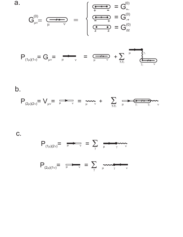
Figure 2: (a) Definition of the effective Green functions $P_{(1\mu)(1\nu)}=G_{\mu\nu}$ via the bare two-site Green functions $G^{(0)}_{\mu\nu}$. (b) Definition of effective interaction lines $P_{(2\mu)(2\nu)}=V_{\mu\nu}$. (c) Definition of intersecting terms $P_{(1\mu)(2\nu)}$, $P_{(2\mu)(1\nu)}$.

The $\cal P$-matrix consists of the two-site effective Green functions ${\cal G}=\|G_{\mu\nu}\|$ $=$ ${\cal G}^{(0)}({\cal E}-{\cal V}^{(0)}{\cal G}^{(0)})^{-1}$, where $G_{\mu\nu}=P_{(1\mu)(1\nu)}$, effective interactions ${\cal V}=\|V_{\mu\nu}\|$ $=$ ${\cal V}^{(0)}({\cal E}-{\cal G}^{(0)}{\cal V}^{(0)})^{-1}$, where $V_{\mu\nu}=P_{(2\mu)(2\nu)}$, and intersecting terms $P_{(1\mu)(2\nu)}$, $P_{(2\mu)(1\nu)}$ (figure 2). The effective Green functions, effective interactions and intersecting terms are denoted in diagrams by directed thick lines, empty lines and compositions of the thick line - empty line, respectively. The $\cal P$-matrix determines the spectrum of quasi-particle excitations in the spin ensemble. Spectrum relations for spin excitations are given by the $\cal P$-matrix poles – by zero eigenvalues of the operator $1-\sigma{\cal P}^{(0)}$ or, equivalently, by ${\cal E}-{\cal V}^{(0)}{\cal G}^{(0)}$ under the analytical continuation

$$i\omega_{m}\to\omega+i\varepsilon\mathop{\rm sign}\nolimits\omega$$

$$\delta(\beta\hbar\omega_{m})=\delta_{m0}\to\frac{1}{\beta\hbar(\omega+i\varepsilon\mathop{\rm sign}\nolimits\omega)}\qquad(\varepsilon\to+0).$$ (13)

Since, zero eigenvalues of the operator ${\cal E}-{\cal V}^{(0)}{\cal G}^{(0)}$ can corresponds to different eigenfunctions and can determine different excitation modes, we introduce the spectral parameter $\lambda$ for eigenfunctions $h^{(\lambda)}_{\mu}(\vec{1},\omega_{m})$ of the operator ${\cal E}-{\cal V}^{(0)}{\cal G}^{(0)}$. The spectral parameter $\lambda$ can be discrete or continuous. Taking into account the above-mentioned, we get the equation describing spin-wave excitations

$$h^{(\lambda)}_{\mu}(\vec{1},\omega_{m})-\sum_{{\vec{1}}^{\prime},{\vec{1}}^{\prime\prime},\nu,\rho}V^{(0)}_{\mu\nu}(\vec{1}-{\vec{1}}^{\prime},\omega_{m})\left.G^{(0)}_{\nu\rho}({\vec{1}}^{\prime},{\vec{1}}^{\prime\prime},\omega_{m})h^{(\lambda)}_{\rho}({\vec{1}}^{\prime\prime},\omega_{m})\right|_{i\omega_{m}\to\omega+i\varepsilon{\rm sign}\omega}=0.$$ (14)

3 Spin waves in nanosized magnetic films

3.1 Spin-wave equations for magnetic films

Let us consider spin waves with the wavevector $\vec{q}$ in a normal magnetized film consisted of $N$ monolayers at low temperature. $x$-, $y$-axes are in the monolayer plane and the $z$-axis is normal to monolayers. The external magnetic field $H$ is normal to monolayers and is parallel to the $z$-axis. At low temperature derivatives of the Brillouin function in $B^{[n]}(p)$ in relation (8) tend to 0 exponentially with decreasing temperature. Thus, it follows that diagrams containing blocks with isolated parts can be dropped, the Green function $G^{(0)}_{zz}$ in relation (11) is negligible and only the Green functions $G^{(0)}_{-+}$, $G^{(0)}_{+-}$ are taken into account in equation (14). Indices $\mu$, $\nu$ of interactions $V^{(0)}_{\mu\nu}$ in equation (14) are $\{-,+\}$. We suppose that on monolayers spins are placed on quadratic crystal lattice sites with the lattice constant $a$ and spin orientation is parallel to the $z$-axis. The exchange interaction acts between neighboring spins and is isotropic between spins in monolayers, $2I_{{-}{+}}=2I_{{+}{-}}=I_{zz}=I_{0}$, and between neighboring layers, $2I_{{-}{+}}=2I_{{+}{-}}=I_{zz}=I_{d}$. Then, the Fourier transform of the exchange interaction with respect to the longitudinal lattice variables $\vec{1}_{xy}$ is

$$\tilde{I}(\vec{q},1_{z}-1^{\prime}_{z})=\sum_{\vec{1}_{xy}-\vec{1}^{\prime}_{xy}}I(\vec{1}_{xy}-\vec{1}^{\prime}_{xy},1_{z}-1^{\prime}_{z})\exp[-i\vec{q}(\vec{1}_{xy}-\vec{1}^{\prime}_{xy})]$$

$$=I(0,1_{z}-1^{\prime}_{z})+2I_{0}[\cos(q_{x}a)+\cos(q_{y}a)]\delta_{1_{z}1^{\prime}_{z}},$$

where $\vec{1}_{xy}$, $\vec{1}^{\prime}_{xy}$ are crystal lattice sites in a monolayer, $1_{z}$, $1^{\prime}_{z}$ are $z$-positions of layers, $\vec{q}=(q_{x},q_{y})$ is the longitudinal wavevector in monolayers, $I(0,1_{z}-1^{\prime}_{z})$ is the exchange interaction at $\vec{q}=0$, which is equal to $I_{d}$ between spins of neighboring layers. The corresponding exchange part of the interaction line $V^{(0)}_{\mu\nu}=V^{(exch)}_{\mu\nu}+V^{(dip)}_{\mu\nu}$ (figure 1(d)) is

$$V^{(exch)}_{\mu\nu}(\vec{q},1_{z}-1^{\prime}_{z})=\beta\tilde{I}(\vec{q},1_{z}-1^{\prime}_{z}).$$ (15)

The MDI part $V^{(dip)}_{\mu\nu}$ is determined by the Fourier transform of equation (3)

$$\left(-q^{2}+\frac{\partial^{2}}{\partial z^{2}}\right)\Phi(\vec{q},z-z^{\prime})=S_{a}^{-1}\delta(z-z^{\prime})$$

with the solution

$$\Phi(\vec{q},1_{z}-1^{\prime}_{z})=\left.\Phi(\vec{q},z-z^{\prime})\right|_{z=1_{z},z^{\prime}=1^{\prime}_{z}}=\frac{-1}{2qS_{a}}\exp(-q|1_{z}-1^{\prime}_{z}|),$$ (16)

where $S_{a}=a^{2}$, $q=|\vec{q}|$. According to the solution (16), the corresponding MDI part of the interaction line is

$$V^{(dip)}_{\mu\nu}(\vec{q},1_{z}-1^{\prime}_{z})=\frac{-4\pi\beta(g\mu_{B})^{2}q_{\mu}q_{\nu}}{qS_{a}}\exp(-q|1_{z}-1^{\prime}_{z}|),\qquad(\mu,\nu=\{{-},{+}\}).$$ (17)

where

$$q_{-}=\frac{1}{2}(q_{x}+iq_{y})\qquad q_{+}=\frac{1}{2}(q_{x}-iq_{y})$$

Taking into account relations (15) and (17), from equation (14) we obtain equations for spin-wave modes with the wavevector $\vec{q}$ in $N$-layer magnetic films

$$h^{(\lambda)}_{\mu}(\vec{q},1_{z},\omega_{m})-\sum_{{\vec{1}}^{\prime}_{z}}\left[V^{(0)}_{\mu{-}}(\vec{q},1_{z}-1^{\prime}_{z},\omega_{m})G^{(0)}_{{-}{+}}(1^{\prime}_{z},1^{\prime}_{z},\omega_{m})h^{(\lambda)}_{+}(\vec{q},1^{\prime}_{z},\omega_{m})\right.$$

$$+\left.\left.V^{(0)}_{\mu{+}}(\vec{q},1_{z}-1^{\prime}_{z},\omega_{m})G^{(0)}_{{+}{-}}(1^{\prime}_{z},1^{\prime}_{z},\omega_{m})h^{(\lambda)}_{-}(\vec{q},1^{\prime}_{z},\omega_{m})\right]\right|_{i\omega_{m}\to\omega+i\varepsilon{\rm sign}\omega}=0,$$ (18)

where

$$G^{(0)}_{{{-}{+}\atop({+}{-})}}(1_{z},1^{\prime}_{z},\omega_{m})=\frac{2B(p)\delta_{1_{z}1^{\prime}_{z}}}{p\pm i\beta\hbar\omega_{m}},$$

$\lambda=1,\ldots,N$ is the mode number, $V^{(0)}_{\mu\nu}(\vec{q},1_{z}-1^{\prime}_{z},\omega_{m})=V^{(exch)}_{\mu\nu}(\vec{q},1_{z}-1^{\prime}_{z})+V^{(dip)}_{\mu\nu}(\vec{q},1_{z}-1^{\prime}_{z})$, $\mu,\nu=\{{-},{+}\}$. Eigenvalues of equations (18) give dispersion relations of spin waves. In next sections we find spin-wave dispersion relations for the cases of monolayer and two-layer films and spin-wave resonance relations for the case of $N$-layer structures.

3.2 Spin waves in magnetic monolayer

Dispersion relations of spin waves in normal magnetized monolayer are determined by the determinant of equations (18) for variables $h^{(1)}_{-}$, $h^{(1)}_{+}$. Taking into account relations (15) and (17), we find

$$\omega^{2}(\vec{q})=\Omega(\vec{q})[\Omega(\vec{q})+2\pi\gamma\sigma_{m}q],$$ (19)

where

$$\Omega(\vec{q})=\gamma(H+H^{(m)})+\frac{2B(p)I_{0}}{\hbar}[2-\cos(q_{x}a)-\cos(q_{y}a)],$$

$\gamma=g\mu_{B}/\hbar$ is the gyromagnetic ratio, $H^{(m)}$ is the depolarizing magnetic field (10), $\sigma_{m}=g\mu_{B}B(p)/S_{a}$ is the surface magnetic moment density, $q=(q_{x}^{2}+q_{y}^{2})^{1/2}$. As one can see from relation (19), in monolayer films spin waves have the one-mode character. Figure 3 presents the dispersion curve (19) of spin waves propagating in the monolayer film with the lattice constant $a=$ 0.4 nm. The spin-wave wavevector $\vec{q}$ is parallel to the $x$-axis ($q_{x}=q$, $q_{y}=0$) and is in the range $[0,\pi/a]$. Calculations have been done for the exchange interaction between neighboring spins $I_{0}=$ 0.085 eV, $B(p)=1/2$ at the sum of magnetic fields $H+H^{(m)}=$ 3 kOe. The exchange interaction makes a major contribution to the dispersion. The relatively weak MDI is significant for the dispersion at small values of the wavevector $\vec{q}$.

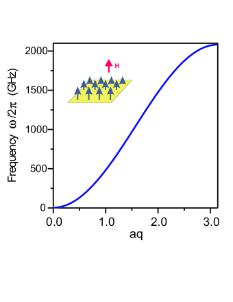
Figure 3: Dispersion curve of spin waves propagating in the normal magnetized monolayer film with cubic lattice ($a=$ 0.4 nm) at the sum of magnetic fields $H+H^{(m)}=$ 3 kOe. Exchange interaction $I_{0}$ is 0.085 eV.

3.3 Spin waves in two-layer magnetic film

Let us consider spin waves in a normal magnetized structure consisted of two monolayers of the quadratic lattice with the lattice constant $a$. The distance between layers is equal to $d$ and the exchange interaction between spins of layers is $I_{d}$. Dispersion relations are determined by eigenvalues of equations (18) for variables $h^{(1)}_{-}$, $h^{(1)}_{+}$, $h^{(2)}_{-}$, $h^{(2)}_{+}$ and can be written as

$$\omega^{(n)2}(\vec{q})=\Omega(\vec{q})[\Omega(\vec{q})+2\pi\gamma\sigma_{m}q]+\frac{2B(p)I_{d}}{\hbar}\left[\frac{2B(p)I_{d}}{\hbar}-2\pi\gamma\sigma_{m}q\exp(-qd)\right]$$

$$\pm 2\left[-\frac{2B(p)I_{d}}{\hbar}(\Omega(\vec{q})+\pi\gamma\sigma_{m}q)+\pi\gamma\sigma_{m}q\exp(-qd)\Omega(\vec{q})\right],$$ (20)

where

$$\Omega(\vec{q})=\gamma(H+H^{(m)})+\frac{2B(p)I_{0}}{\hbar}[2-\cos(q_{x}a)-\cos(q_{y}a)]+\frac{B(p)I_{d}}{\hbar},$$

$n=1,2$ is the mode number, $q=(q_{x}^{2}+q_{y}^{2})^{1/2}$. For the first mode spins in different layers change their orientations in-phase. In this case, spin waves of the first mode correspond to spin waves in monolayer (19). For the second mode spins in different layers change orientations in-anti-phase and the energy of the spin wave with the given longitudinal wavevector $q$ is higher than the energy of the spin wave of the first mode. Dispersion curves of spin waves determined by relations (20) are shown in figure 4. Spin waves propagate along the $x$-axis. Calculations have been done for the exchange interactions $I_{0}=I_{d}=$ 0.085 eV and for the distance between layers $d=a=$ 0.4 nm at the sum of magnetic fields $H+H^{(m)}=$ 3 kOe.

Figure 4: Dispersion curve of spin waves propagating in the normal magnetized two-layer magnetic film with quadratic lattice ($a=$ 0.4 nm) at the sum of magnetic fields $H+H^{(m)}=$ 3 kOe. Exchange interactions $I_{0}=I_{d}=$ 0.085 eV. Distance between monolayers $d$ is equal to the lattice constant $a$. 1, 2 are the first and the second modes of spin waves, respectively.

3.4 Spin-wave resonance in $N$-layer structure

In this section we consider spin-wave resonance in a structure consisted of $N$ uniform monolayers with the exchange interaction $I_{d}$ between spins of layers and with the distance $d$ between layers. Spin-wave resonance is the limit case of a spin wave, when the longitudinal wavevector $q\rightarrow 0$. Therefore, the MDI terms $V^{(dip)}_{\mu\nu}(\vec{q},1_{z}-1^{\prime}_{z})$ in equations (18) can be dropped, equations with variables $h_{+}^{(\lambda)}$ and $h_{-}^{(\lambda)}$ are separated and eigenvalues are determined by zero values of the determinant (we write the determinant ${\cal D}^{(+)}$ for equations with the $h_{+}^{(\lambda)}$)

$${\cal D}^{(+)}=G^{(0)}(1)\ldots G^{(0)}(N)$$

$$\times\det\left(\begin{array}[]{cccc}(G^{(0)-1}(1)-V^{(0)}(11))&-V^{(0)}(12)&0&\vdots\\ -V^{(0)}(21)&(G^{(0)-1}(2)-V^{(0)}(22))&-V^{(0)}(23)&\vdots\\ 0&-V^{(0)}(32)&(G^{(0)-1}(3)-V^{(0)}(33))&\vdots\\ \cdots&\cdots&\cdots&\cdots\end{array}\right),$$

where $V^{(0)}(ij)$, $G^{(0)}(i)$ are the abridged notation of $V^{(exch)}_{{+}{-}}(\vec{q},i_{z}-j_{z},\omega_{m})|_{\vec{q}=0}$ and $G^{(0)}_{{-}{+}}(i,i,\omega_{m})$ at ${i\omega_{m}\to\omega+i\varepsilon{\rm sign}\omega}$, respectively. $(i,j)$ are indices of layers. Taking into account that spins of outer layers ($i=1,N$) interact with spins of one inner layer and spins of inner layers interact with spins of two layers and introducing the variable for inner layers in the determinant ${\cal D}^{(+)}$

$$x=\frac{G^{(0)-1}(i)-V^{(0)}(ii)}{-V^{(0)}(ji)}=\frac{\hbar}{B(p)I_{d}}[\omega-\gamma(H+H^{(m)})]-2\qquad(i\neq 1,N,\quad j=i\pm 1),$$

we obtain that the spin-wave resonance spectrum is determined by roots of the polynomial

$$R_{N}(x)=\left|\begin{array}[]{ccccccc}(x+1)&1&0&0&\vdots&0&0\\ 1&x&1&0&\vdots&0&0\\ 0&1&x&1&\vdots&0&0\\ 0&0&1&x&\vdots&0&0\\ \cdots&\cdots&\cdots&\cdots&\cdots&\cdots&\cdots\\ 0&0&0&0&\vdots&x&1\\ 0&0&0&0&\vdots&1&(x+1)\end{array}\right|$$

$$=(x+1)^{2}P_{N-2}(x)-2(x+1)P_{N-3}(x)+P_{N-4}(x)=0\qquad(N\geq 2),$$

where $P_{-2}(x)=-1$, $P_{-1}(x)=0$, $P_{0}(x)=1$, $P_{N}(x)=xP_{N-1}(x)-P_{N-2}(x)$. Polynomial $R_{N}(x)$ has $N$ roots

$$x^{(n)}=-2\cos\left(\frac{\pi n}{N}\right),$$

where $n=0,1,\ldots,N-1$. Taking into account the form of the roots $x^{(n)}$, we can introduce the transverse wavevector $q_{z}^{(n)}=\pi n/Nd$. Then, the spin-wave resonance spectrum can be written as

$$\omega^{(n)}=\gamma(H+H^{(m)})+\frac{2B(p)I_{d}}{\hbar}[1-\cos(q_{z}^{(n)}d)].$$ (21)

For the first mode ($n=0$) spins in different layers change their orientations in-phase. For the highest mode ($n=N-1$) spins in different layers change orientations in-anti-phase and the energy of spin-wave resonance is highest. Figure 5 presents the spin-wave resonance spectrum for the structure with $N=40$ layers. One can see that at low values of the transverse wavevector the resonance spectrum is proportional to the quadratic dependence on $q_{z}^{(n)}$.

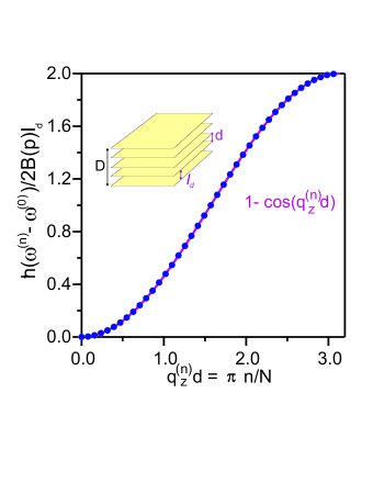
Figure 5: Spin-wave resonance spectrum $\omega^{(n)}$ ($n=0,1,\ldots,N-1$) for the structure with $N=40$ layers. $q_{z}^{(n)}$ is the transverse wavevector, $d$ is the distance between layers, $I_{d}$ is the exchange interaction between spins of layers.

4 Landau-Lifshitz equations and spin-wave excitations in thick magnetic films

4.1 Linearized Landau-Lifshitz equations

Equations (14), (18) describe spin-wave excitations. Solutions of these equations for magnetic samples of great volumes and for thick $N$-layer magnetic films with $N\gg 1$ become difficult, because determinants of equations (14), (18) have high orders. In order to overcome the difficulty and to find spin-wave spectrum for these samples, we derive Landau-Lifshitz equations [17, 18]. Dispersion relations for spin excitations are determined by the $\cal P$-matrix poles (12) which coincide with poles of the matrix ${\cal G}$ of effective propagators. Accordingly, the dispersion relations can be derived from the eigenvalues of equation

$${\cal G}={\cal G}^{(0)}+{\cal G}({\cal V}^{({\rm exch})}+{\cal V}^{({\rm dip})}){\cal G}^{(0)},$$ (22)

where ${\cal G}^{(0)}=\|G^{(0)}_{\mu\nu}\|$ is the matrix of bare propagators (11). Since the considered interaction is the sum of exchange and magnetic dipole interactions, we can obtain the eigenvalues and eigenfunctions of equation (22) by a two-step procedure. In the first stage, we perform the summation of diagrams, taking into account the exchange interaction, and find the propagator matrix ${\cal G}^{(1)}=\|G^{(1)}_{\mu\nu}\|$

$${\cal G}^{(1)}={\cal G}^{(0)}+{\cal G}^{(0)}{\cal V}^{({\rm exch})}{\cal G}^{(1)}.$$ (23)

In the second stage, the summation of diagrams with dipole interaction lines is performed. This gives the equation for the matrix ${\cal G}$ of effective propagators expressed in terms of the matrix ${\cal G}^{(1)}$

$${\cal G}={\cal G}^{(1)}+{\cal G}{\cal V}^{({\rm dip})}{\cal G}^{(1)}.$$ (24)

Thus, the solution of equation (22), which determines the matrix ${\cal G}$, is equivalent to the solution of equations (23), (24). After the performed two-step summation, equation (14) for eigenfunctions $h^{(\lambda)}_{\mu}$ is written in the more convenient form

$$h^{(\lambda)}_{\mu}(\vec{1},\omega_{m})-\left.\sum_{\rho,\sigma\atop\vec{1^{\prime}}\vec{1^{\prime\prime}}}V^{({\rm dip})}_{\mu\rho}(\vec{1}-\vec{1^{\prime}},\omega_{m})G^{(1)}_{\rho\sigma}(\vec{1^{\prime}},\vec{1^{\prime\prime}},\omega_{m})h^{(\lambda)}_{\sigma}(\vec{1^{\prime\prime}},\omega_{m})\right|_{i\omega_{m}\to\omega+i\varepsilon{\rm sign}\omega}=0.$$ (25)

The solution of simultaneous equations (23), (25) gives the dispersion relations for spin excitations. These equations can be reduced to linearized Landau-Lifshitz equations in the generalized form and the equation for the magnetostatic potential. In order to perform this transformation one needs to make a transition to the retarded Green functions. We transform matrix equation (23) to equations describing small variations of the magnetic moment density (or the variable magnetization), $m_{\nu}$. The variable magnetization $m_{\nu}$ under the action of the magnetic field $\bar{h}_{\nu}$, which is generated by the MDI ${\cal V}^{({\rm dip})}$, is given by the retarded Green functions, which are determined by the analytical continued values of the propagator matrix ${\cal G}^{(1)}$ [31]

$$m_{\nu}(\vec{1},\omega)=\frac{\beta(g\mu_{B})^{2}}{V_{a}}\left.\sum_{\rho,\vec{1^{\prime}}}G^{(1)}_{\nu\rho}(\vec{1},\vec{1^{\prime}},\omega_{m})\right|_{i\omega_{m}\to\omega-i\varepsilon}\bar{h}_{\rho}(\vec{1^{\prime}},\omega),$$ (26)

where $V_{a}$ is the atomic volume. The analytical continuation $i\omega_{m}\to\omega-i\varepsilon$ defines the retarded Green functions. $\bar{h}_{\rho}(\vec{1},\omega)$ is the field of the magnetic dipole-dipole interaction acting on spins. By multiplying matrix equation (23) by ${\cal G}^{(0)-1}$ from the left and by $\bar{h}_{\rho}$ from the right, performing the analytical continuation $i\omega_{m}\to\omega-i\varepsilon$, $\delta(\beta\hbar\omega_{m})\to[\beta\hbar(\omega-i\varepsilon)]^{-1}$ and taking into account relation (26), we get matrix equation (23) in the form of simultaneous equations

$$\sum_{\nu,\vec{1^{\prime}}}[G^{(0)-1}_{\rho\nu}(\vec{1},\vec{1^{\prime}},\omega)-\beta I_{\rho\nu}(\vec{1}-\vec{1^{\prime}})]m_{\nu}(\vec{1^{\prime}},\omega)=\frac{\beta(g\mu_{B})^{2}}{V_{a}}\bar{h}_{\rho}(\vec{1},\omega).$$ (27)

For isotropic exchange interaction, $2I_{{-}{+}}=2I_{{+}{-}}=I_{zz}=I$, equations (27) have the form

$$\hat{E}_{\pm}m_{\pm}(\vec{1},\omega)=2\gamma M(\vec{1})\bar{h}_{\mp}(\vec{1},\omega)$$ (28)

$$\hat{E}_{z}m_{z}(\vec{1},\omega)=\frac{B^{[1]}(p)}{B(p)}\gamma M(\vec{1})\bar{h}_{z}(\vec{1},\omega),$$ (29)

where $M(\vec{1})=g\mu_{B}B(p)/V_{a}$ is the magnetic moment density at the low-temperature approximation. We say that the operators $\hat{E}_{\pm}$, $\hat{E}_{z}$:

$$\hat{E}_{\pm}m_{\pm}(\vec{1},\omega)=[\gamma(H(\vec{1})+H^{(m)}(\vec{1}))\pm\omega]m_{\pm}(\vec{1},\omega)$$

$$+\frac{B(p)}{\hbar V_{b}}\sum_{\vec{1^{\prime}}}\int\limits_{V_{b}}[\bar{I}(0)-\bar{I}(\vec{q})]\exp[i\vec{q}(\vec{1}-\vec{1^{\prime}})]m_{\pm}(\vec{1^{\prime}},\omega)\,d^{3}q$$

$$\hat{E}_{z}m_{z}(\vec{1},\omega)=\omega m_{z}(\vec{1},\omega)-\frac{B^{[1]}(p)}{\hbar V_{b}}\sum_{\vec{1^{\prime}}}\int\limits_{V_{b}}\bar{I}(\vec{q})\exp[i\vec{q}(\vec{1}-\vec{1^{\prime}})]m_{z}(\vec{1^{\prime}},\omega)\,d^{3}q$$

are Landau-Lifshitz operators. $\bar{I}(\vec{q})=\sum_{\vec{1}}I(\vec{1})\exp(-i\vec{q}\vec{1})$ is the Fourier transform of the exchange interaction with respect to the lattice variables. The field $H^{(m)}(\vec{1})$ is defined by relation (10) and depends on the magnetic moment density $M(\vec{1})$; $V_{b}=(2\pi)^{3}/V_{a}$ is the volume of the first Brillouin zone. Equations (28), (29) have the generalized form of the Landau-Lifshitz equations [13]. Solutions $m_{\pm}$ of equations (28) depend on temperature, because $\beta=1/kT$ is contained in the variable $p$ of the function $B(p)$ (8), through which the magnetic moment density $M(\vec{1})$ is expressed. Equation (29) describes longitudinal variations of the variable magnetization under the influence of the field $\bar{h}_{z}$. At low temperature the derivative of the function $B^{[1]}(p)$ tends to 0 and the longitudinal variable magnetization $m_{z}$ is negligible.

From the form of the magnetic dipole interaction in relations (2), (3) it follows that the field $\bar{h}_{\nu}$ in relation (26) is magnetostatic, i.e. it is expressed in terms of the magnetostatic potential $\varphi$: $\bar{h}_{\nu}=-\nabla_{\nu}\varphi$. We transform equation (25) to the equation for the magnetostatic potential $\varphi(\vec{r},\omega)$. Taking into account relation (26) and the explicit form of the magnetic dipole interaction in relations (2), (3), performing the derivation $\nabla_{\mu}$, the analytical continuation $i\omega_{m}\to\omega-i\varepsilon$ and the summation of equation (25) over the index $\mu$, we obtain the equation expressed in terms of $\varphi$, $m_{\nu}$

$$-\Delta\varphi(\vec{r},\omega)+4\pi\nabla_{\nu}m_{\nu}(\vec{1},\omega)|_{\vec{1}\to\vec{r}}=0.$$ (30)

Thus, in consideration of the Landau-Lifshitz equations (28), (29), the dispersion relations of spin excitations are given by eigenvalues of equation (30).

4.2 Exchange boundary conditions

If the scale of the spatial distribution of the variable magnetization $m_{\nu}(\vec{1},\omega)$ and the sample size are much greater than the lattice constant $a$, then the sum over the lattice variables $\sum_{\vec{1}}$ in Landau-Lifshitz operators $\hat{E}_{\pm}$, $\hat{E}_{z}$ can be converted into an integral over the sample volume $V_{a}^{-1}\int\,d^{3}r$. Let us consider the case when the temperature is low and the Fourier transform of the exchange interaction is $\bar{I}(\vec{q})=\bar{I}(0)-wq^{2}$. Then, we obtain that $m_{z}\to 0$ and equation (29) is dropped. The operators $\hat{E}_{\pm}$ are pseudodifferential operators of order 2 [32]

$$\hat{E}_{\pm}m_{\pm}(\vec{r},\omega)=[\gamma(H(\vec{r})+H^{(m)}(\vec{r}))\pm\omega]m_{\pm}(\vec{r},\omega)$$

$$+\frac{4\pi\gamma\alpha M(\vec{r})}{(2\pi)^{3}}\int\limits_{V}\int\limits_{V_{b}}q^{2}\exp[i\vec{q}(\vec{r}-\vec{r^{\prime}})]m_{\pm}(\vec{r^{\prime}},\omega)\,d^{3}q\,d^{3}r,$$ (31)

where $\alpha=wV_{a}/4\pi(g\mu_{B})^{2}$ is the exchange interaction constant, $V$ is the volume of the ferromagnetic sample. In [10, 11, 12, 13, 33, 34, 35, 36, 37] the pseudodifferential Landau-Lifshitz operators are reduced to the differential operators with respect to spatial variables

$$\hat{E}_{\pm}(\vec{r},\omega)=\gamma[H(\vec{r})+H^{(m)}(\vec{r})-4\pi\alpha M(\vec{r})\Delta]\pm\omega.$$ (32)

For solvability of equations (28) with differential Landau-Lifshitz operators (32) the exchange boundary conditions are imposed

$$\frac{\partial m_{\nu}}{\partial\vec{n}}+\xi m_{\nu}|_{\partial V}=0,$$

where $\vec{n}$ is the inward normal to the boundary $\partial V$, and $\xi$ is the pinning parameter. This reduction to differential Landau-Lifshitz operators is not correct. Figure 6 presents exact dispersion relations of spin excitations given by eigenvalues of equations (28), (30) with pseudodifferential and differential Landau-Lifshitz operators for the case of a normal magnetized homogeneous film with the thickness $D$. The dispersion relations of spin waves have the form

$$\omega^{(n)2}(\vec{q})=\Omega^{(n)}(\Omega^{(n)}+\Omega_{M}q^{2}/q^{(n)2}_{0}),$$ (33)

where $n=1,2,3,\ldots$ is the mode number, $\vec{q}=(q_{x},q_{y})$ is the two-dimensional longitudinal wavevector of spin waves, $q=|\vec{q}|$, $\Omega^{(n)}=\gamma(H-4\pi M+4\pi\alpha Mq^{(n)2}_{0})$, $\Omega_{M}=4\pi\gamma M$, $q^{(n)}_{0}=(q^{2}+q^{(n)2}_{z})^{1/2}$, $q_{z}^{(n)}$ is the transverse vector. The magnetostatic potential over thickness $z\in[-D/2,D/2]$ of the magnetic film is

$$\varphi^{(n,\vec{q})}(x,y,z)=(2\pi)^{-1}f^{(n)-1/2}\exp(iq_{x}x+iq_{y}y)\cos[q^{(n)}_{z}z+\pi(n-1)/2],$$ (34)

where $f^{(n)}=D/2+q/q^{(n)2}_{0}$.

For the case of pseudodifferential Landau-Lifshitz operators (31), the transverse wavevector $q^{(n)}_{z}$ is closely connected to the longitudinal wavevector $q$ by the relation

$$2\cot q^{(n)}_{z}D=\frac{q^{(n)}_{z}}{q}-\frac{q}{q^{(n)}_{z}}.$$ (35)

For the case of differential Landau-Lifshitz operators (32), the transverse wavevector is determined by the exchange boundary conditions and is given by the equation [10, 13]

$$2\cot q^{(n)}_{z}D=\frac{q^{(n)}_{z}}{\xi}-\frac{\xi}{q^{(n)}_{z}}.$$ (36)

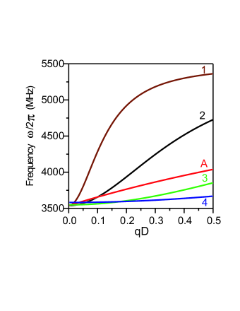
Figure 6: Dispersion curves of the first spin-wave mode propagating in the YIG film of the thickness $D=$ 0.5 $\mu$m with $4\pi M=$ 1750 Oe, $\alpha=$ 3.2$\cdot$10^-12 cm² at the applied magnetic field $H=$ 3000 Oe. The curve $A$ is calculated on the base of relation (35) for the case of pseudodifferential Landau-Lifshitz operators (31). Curves 1 - 4 are calculated for the case of differential Landau-Lifshitz operators (32) on the base of relation (36) with different pinning parameters $\xi$. (1) $\xi D$ = 0.01, (2) 0.1, (3) 1, (4) 10.

Dispersion relations (33) of the first spin-wave mode propagating in the YIG film of the thickness $D=$ 0.5 $\mu$m with $4\pi M=$ 1750 Oe, $\alpha=$ 3.2$\cdot$10^-12 cm² at the applied magnetic field $H=$ 3000 Oe are shown in figure 6 for the transverse wave vector $q^{(1)}_{z}$ (35) and for the transverse wave vector $q^{(1)}_{z}$ (36) with different pinning parameters $\xi$. One can see that there does not exist any pinning parameter $\xi$, at which the curve $A$ calculated on the base of relation (35) coincides with the curves calculated on the base of the exchange boundary conditions. Thus, we conclude that the reduction to differential Landau-Lifshitz operators and the use of the exchange boundary conditions are incorrect.

5 Spin-wave relaxation

In this section we answer the question: what is the value of spin-wave relaxation in the model with magnetic dipole and exchange interactions derived from first principles? The answer depends on the ratio of the spin-wave energy to intervals between modes of the spin-wave spectrum and is different for thick and for thin magnetic films. In thick films the spin-wave energy is greater than energy gaps between modes and a three-spin-wave process takes place. If the exchange interaction is isotropic, it cannot induce three-magnon processes and, therefore, the MDI makes a major contribution to the relaxation. We consider the spin-wave damping in thick films in the one-loop approximation. In thin magnetic films (for example, in nanosized films) the energy of long-wavelength spin waves is less than energy gaps between modes and three-spin-wave processes are forbidden. In this case, four-spin-wave processes take place, the exchange interaction makes a major contribution to the relaxation, and the spin-wave damping has lower values in comparison with the damping in thick films. We calculate the spin-wave relaxation for four-spin-wave processes in thin films for long-wavelength spin waves in the two-loop approximation.

5.1 Spin-wave relaxation in thick films

The spin-wave relaxation induced by a three-spin-wave process in normal magnetized homogeneous ferromagnetic films is considered in [17, 18] in the one-loop approximation for spin waves with small longitudinal wavevectors at low temperature. The relaxation is determined by self-energy diagram insertions $\Sigma_{(1{+})(1{-})}$ to the $\cal P$-matrix given by relation (12) (figure 7). Damping of the $j$-mode excitation is defined by the imaginary part of the pole of the effective Green functions $G_{-+}=P_{(1{-})(1{+})}$ with insertions $\Sigma_{(1{+})(1{-})}$ under the analytical continuation (13)

$$\Delta^{(j)}(\vec{q})=\frac{\delta\omega^{(j)}(\vec{q})}{\omega^{(j)}(\vec{q})}=\left.\frac{2B(p)V_{a}}{\beta\hbar\omega^{(j)}(\vec{q})}\mathop{\rm Im}\nolimits\Sigma_{(1{+})(1{-})}(j,j,\vec{q},\omega_{m})\right|_{i\omega_{m}\to\omega+i\varepsilon\mathop{\rm sign}\nolimits\omega}$$

$$=\frac{V_{a}}{2\beta\hbar\omega^{(j)}}\mathop{\rm Im}\nolimits\sum_{n,i,k}\int F^{(i)}F^{(k)}[\bar{P}_{(1{-})(1{+})}(i,-\vec{q}_{1},-\omega_{n})\bar{P}_{(2z)(2z)}(k,\vec{q}-\vec{q}_{1},\omega_{m}-\omega_{n})$$

$$+\left.\frac{1}{8B(p)}\bar{P}_{(1{-})(2z)}(i,\vec{q}_{1},\omega_{n})\bar{P}_{(2z)(1{+})}(k,\vec{q}-\vec{q}_{1},\omega_{m}-\omega_{n})]N^{2}(j,\vec{q};i,\vec{q}_{1};k,\vec{q}-\vec{q}_{1})\,d^{2}q_{1}\right|_{i\omega_{m}\to\omega+i\varepsilon\mathop{\rm sign}\nolimits\omega},$$ (37)

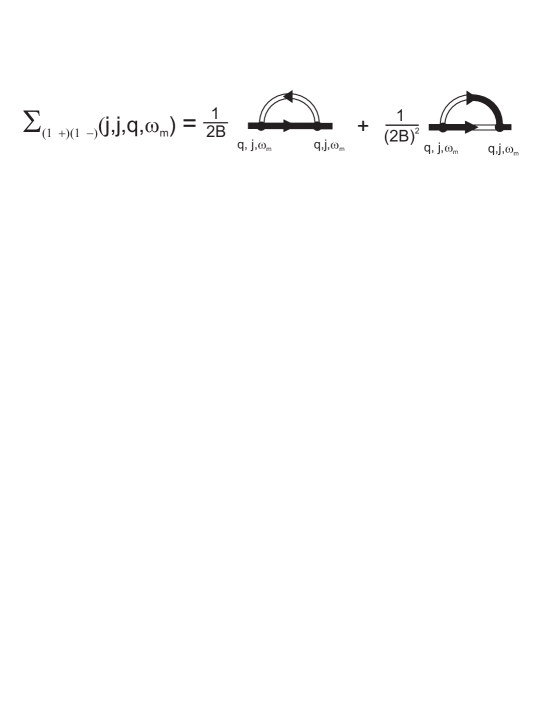
Figure 7: Self-energy diagrams in the one-loop approximation at low temperature. $B$ is determined by relation (8).

where

$$\bar{P}_{(1{-})(1{+})}(j,\vec{q},\omega_{m})=2\rho V_{a}^{2}(\Omega^{(j)}+2\eta^{(j)}_{{-}{+}}+i\omega_{m})$$

$$\bar{P}_{(1{-})(2z)}(j,\vec{q},\omega_{m})=-2\eta^{(j)}_{{+}{z}}(\Omega^{(j)}+i\omega_{m})$$

$$\bar{P}_{(2z)(1{+})}(j,\vec{q},\omega_{m})=-2\eta^{(j)}_{z{-}}(\Omega^{(j)}+i\omega_{m})$$

$$\bar{P}_{(2z)(2z)}(j,\vec{q},\omega_{m})=F^{(j)-1}\beta V_{a}\tilde{I}(q_{0}^{(j)})-\rho^{-1}\eta^{(j)}_{{z}{z}}(\Omega^{(j)2}+i\omega_{m}^{2})$$

$$F^{(j)}=(\omega^{(j)2}+\omega^{2}_{m})^{-1},\qquad\rho=\frac{B(p)}{\beta\hbar V_{a}},$$

$$\eta^{(j)}_{\mu\nu}=\frac{\Omega_{M}q_{\mu}q_{\nu}}{q^{(j)2}_{0}}\qquad(\mu,\nu={-},{+},z)$$

$$q_{\pm}=\frac{1}{2}(q_{x}\mp iq_{y}),$$

$$\tilde{I}(q_{0}^{(j)})=\tilde{I}(0)-wq^{(j)2}_{0}.$$

is the Fourier transform of the exchange interaction,

$$N(j_{1},\vec{q_{1}};j_{2},\vec{q_{2}};j_{3},\vec{q_{3}})$$

$$=\frac{1}{8\pi V_{a}}\prod^{3}_{k=1}\frac{1}{f^{(j_{k})1/2}}\sum_{\sigma_{1},\sigma_{2},\sigma_{3}}\frac{\sin\left[\left(\sum^{3}_{k=1}\sigma_{k}q^{(j_{k})}_{z}\right)D/2\right)]}{\sum^{3}_{k=1}\sigma_{k}q^{(j_{k})}_{z}}\exp\left(i\sum^{3}_{k=1}\sigma_{k}\pi{(j_{k}-1)/2}\right)$$

is the block factor in the representation of the functions (34), $f^{(j)}=D/2+q/q_{0}^{(j)2}$, $\sigma_{k}=\pm 1$; $\sum_{\sigma_{1},\sigma_{2},\sigma_{3}}$ denotes the summation over all sets $\{\sigma_{1},\sigma_{2},\sigma_{3}\}$. The spin-wave frequency $\omega^{(j)}$ and the transverse wavevector $q^{(j)}_{z}$ are determined by relations (33) and (35), respectively. The damping $\Delta^{(j)}$ increases directly proportionally to the temperature.

Relation (37) describes relaxation of the spin-wave $j$-mode caused by inelastic scattering on thermal excited spin wave modes. Relaxation occurs through the confluence of the $j$-mode with the $k$-mode to form the $i$-mode. From the explicit form of the block factor $N$ in relation (37) it follows that the confluence processes take place when the sum of mode numbers $j+i+k$ is equal to an odd number. The confluence processes are induced by the MDI and are accompanied by transitions between thermal excited $i$- and $k$-modes. Transitions take place when equation

$$\omega^{(j)}(\vec{q})=\omega^{(i)}({\vec{q}}{\,}^{(s)})-\omega^{(k)}(\vec{q}-{\vec{q}}{\,}^{(s)})$$ (38)

has at least one solution ${\vec{q}}{\,}^{(s)}$ for the given ${\vec{q}}$, $i$, $j$,$k$. Existence of solutions ${\vec{q}}{\,}^{(s)}$ of equation (38) depends on the thickness of the magnetic film. With decreasing film thickness $D$, the density of dispersion curves of modes on the plane $(\omega,q)$ decreases and the frequency of the spacings between curves increase. The least frequency spacing occurs between the first ($i=1$) and the third ($k=3$) modes. Figure 8 shows the damping $\Delta^{(1)}$ of the first spin wave mode versus the longitudinal wave vector $q$ normalized by the film thickness $D$ at different film thicknesses. Calculations have been done for a YIG film with the magnetization $4\pi M=$ 1750 Oe and the exchange interaction constant $\alpha=$ 3.2$\cdot$10^-12 cm² at $H=$ 3000 Oe and $T=$ 300 K. One can see that for the YIG film with the thickness $D=$ 120 nm in the region $qD<0.14$ the damping $\Delta^{(1)}$ is equal to 0 due to the absence of transitions between modes. Thus, in thin magnetic films a low spin-wave relaxation region takes place. For the given $j$-mode this region appears, when the excitation frequency $\omega^{(j)}(\vec{q})$ is less than the difference $\omega^{(3)}({\vec{q}}{\,}^{(s)})-\omega^{(1)}(\vec{q}-{\vec{q}}{\,}^{(s)})$ at any values of the wavevector ${\vec{q}}{\,}^{(s)}$. For the first mode $\omega^{(1)}$ in the YIG film the low spin-wave relaxation region is shown in figure 9 at $q\to 0$. If the film thickness $D<D_{0}(\omega^{(1)}/2\pi)$, then $\omega^{(1)}(0)<\omega^{(3)}({\vec{q}}{\,}^{(s)})-\omega^{(1)}({\vec{q}}{\,}^{(s)})$ and the first mode has low values of the spin wave damping $\Delta^{(1)}$.

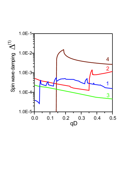
Figure 8: Spin wave damping $\Delta^{(1)}={\delta\omega^{(1)}}/{\omega^{(1)}}$ of the first mode in normal magnetized YIG film with the magnetization $4\pi M=$ 1750 Oe and the exchange interaction constant $\alpha=$ 3.2$\cdot$10^-12 cm² at $H=$ 3000 Oe, $T=$ 300 K at different film thickness $D$. (1) $D=$ 500 nm, (2) 300 nm, (3) 200 nm, (4) 120 nm.

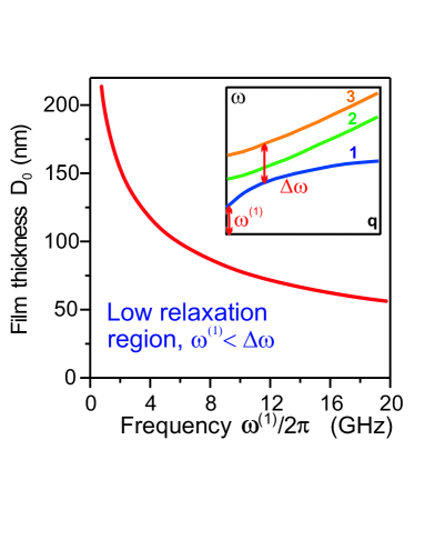
Figure 9: Film thickness $D_{0}$ of YIG film versus the excitation frequency $\omega^{(1)}(\vec{q})/2\pi$ of the first mode at the wavevector $\vec{q}\to 0$. Low relaxation region of the first spin-wave mode exists for YIG films with the thickness $D<D_{0}(\omega^{(1)}/2\pi)$.

5.2 Relaxation in thin magnetic films

What is the value of spin wave damping in the low relaxation region in thin magnetic films? We consider four-spin-wave processes in the normal magnetized monolayer of the quadratic lattice with the lattice constant $a$ at small longitudinal wavevector values $\vec{q}=(q_{x},q_{y})$ at low temperature. As isotropy of the exchange interaction can not forbid four-spin-wave processes and the value of the exchange interaction much greater than the MDI, only the exchange interaction will be taken into account in diagrams. We suppose that the exchange interaction acts between neighboring spins and is equal to $I_{0}$. In order to calculate self-energy diagram insertions to the effective Green functions in the two-loop approximation, we use the ladder expansion (figure 10). At small values of wavevectors the bare $\Gamma_{0}$-vertex (figure 10a) is

$$\Gamma_{0}(1,2;3,4)\equiv\Gamma_{0}(\vec{k},\vec{s}+\vec{q}-\vec{k};\vec{q},\vec{s})$$

$$=\beta[\tilde{I}(\vec{k}-\vec{q})+\tilde{I}(\vec{k}-\vec{s})-\tilde{I}(\vec{s})-\tilde{I}(\vec{q})]=2\beta I_{0}a^{2}(\vec{q},\vec{s}),$$

where $1,2;3,4$ is the abridged notation of 2-dimensional wavevectors, which are variables of $\Gamma_{0}$-vertex; $|\vec{k}|,|\vec{q}|,|\vec{s}|\ll a^{-1}$;

$$\tilde{I}(\vec{q})=\sum_{\vec{1}_{xy}-\vec{1}^{\prime}_{xy}}I(\vec{1}_{xy}-\vec{1}^{\prime}_{xy})\exp[-i\vec{q}(\vec{1}_{xy}-\vec{1}^{\prime}_{xy})]=2I_{0}[\cos(q_{x}a)+\cos(q_{y}a)].$$

The $\Gamma$-vertex in the ladder approximation (figure 10b) is determined by the relationship

$$\Gamma(1,2;3,4)\equiv\Gamma(\vec{k},\omega_{1},\vec{s}+\vec{q}-\vec{k},\omega_{3}+\omega_{4}-\omega_{1};\vec{q},\omega_{3},\vec{s},\omega_{4})=\Gamma_{0}(\vec{k},\vec{s}+\vec{q}-\vec{k};\vec{q},\vec{s})$$

$$+\frac{1}{8B^{2}(p)S_{b}}\sum_{\omega^{(q)}_{m}}\int\Gamma_{0}(\vec{k},\vec{s}+\vec{q}-\vec{k};\vec{q^{\prime}},\vec{s}+\vec{q}-\vec{q^{\prime}})G_{{-}{+}}(\vec{q^{\prime}},\omega^{(q)}_{m})G_{{-}{+}}(\vec{s}+\vec{q}-\vec{q^{\prime}},\omega_{3}+\omega_{4}-\omega^{(q)}_{m})$$

$$\times\Gamma(\vec{q^{\prime}},\omega^{(q)}_{m},\vec{s}+\vec{q}-\vec{q^{\prime}},\omega_{3}+\omega_{4}-\omega^{(q)}_{m};\vec{q},\omega_{3},\vec{s},\omega_{4})\,d^{2}q^{\prime},$$

where

$$G_{{-}{+}}(\vec{q},\omega_{m})=\frac{2B(p)}{\beta\hbar(\omega(\vec{q})-i\omega_{m})}$$

is the effective Green function determined by the ${\cal P}$-matrix (12), $\omega(\vec{q})$ is the frequency of spin excitations in monolayer (19), $S_{b}$ is the volume of the 2-dimensional first Brillouin zone. The coefficient $1/8B^{2}(p)$ is due to the fact that the substitution of the bare Green function to effective ones in diagrams are performed inside blocks. The self-energy diagram insertion (figure 10c) is given by

$$\Pi(\vec{q},\omega^{(q)}_{m})=\frac{1}{2S_{b}}\sum_{\omega^{(k)}_{n}}\int\Gamma_{0}(\vec{q},\vec{k};\vec{q},\vec{k})G_{{-}{+}}(\vec{k},\omega^{(k)}_{n})\,d^{2}k$$

$$+\frac{1}{16B^{2}(p)S_{b}^{2}}\sum_{\omega^{(k)}_{n},\omega^{(s)}_{l}}\int\int\Gamma_{0}(\vec{q},\vec{s}+\vec{k}-\vec{q};\vec{s},\vec{k})G_{{-}{+}}(-\vec{s}-\vec{k}+\vec{q},-\omega^{(k)}_{n}-\omega^{(s)}_{l}+\omega^{(q)}_{m})$$

$$\times G_{{-}{+}}(\vec{k},\omega^{(k)}_{n})G_{{-}{+}}(\vec{s},\omega^{(s)}_{l})\Gamma(\vec{s},\omega^{(s)}_{l},\vec{k},\omega^{(k)}_{n};\vec{q},\omega^{(q)}_{m},\vec{s}+\vec{k}-\vec{q},\omega^{(k)}_{n}+\omega^{(s)}_{l}-\omega^{(q)}_{m})\,d^{2}k\,d^{2}s.$$ (39)

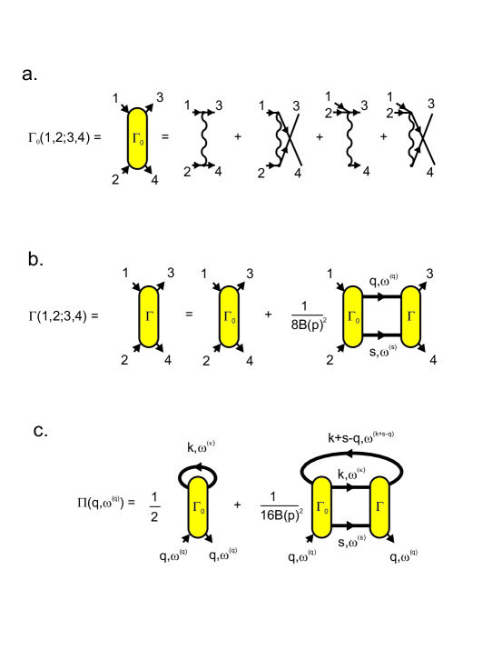
Figure 10: (a) Bare $\Gamma_{0}$-vertex. (b) Ladder approximation. (c) Self-energy diagram insertion.

The damping of spin wave excitations is expressed by the imaginary part of the self-energy $\Pi(\vec{q},\omega^{(q)}_{m})$

$$\Delta(\vec{q})=\frac{\delta\omega(\vec{q})}{\omega(\vec{q})}=\left.\frac{\mathop{\rm Im}\nolimits\Pi(\vec{q},\omega^{(q)}_{m})}{\beta\omega}\right|_{i\omega_{m}\to\omega+i\varepsilon\mathop{\rm sign}\nolimits\omega}.$$ (40)

Taking into account the self-energy $\Pi(\vec{q},\omega^{(q)}_{m})$ in the Born approximation, namely, substituting $\Gamma\rightarrow\Gamma_{0}$ in relation (39), integrating over $\vec{k}$, $\vec{s}$ and summing over the frequency variables $\omega^{(k)}_{n}$ and $\omega^{(s)}_{l}$ in equation (40), at $\hbar\omega(\vec{q})<kT$ we obtain

$$\Delta(\vec{q})=\frac{C(qa)^{2}(kT)^{2}}{16\pi B^{2}(p)I_{0}\varepsilon^{(0)}},$$

where $C=1.12$, $k$ is the Boltzmann constant, $\varepsilon^{(0)}=\hbar\gamma(H+H^{(m)})$ is the Zeeman energy. In order to evaluate the damping of spin waves, we calculate $\Delta(\vec{q})$ for spin waves with the wavelength $\lambda=$ 5 $\mu$m propagating in the monolayer film with the lattice constant $a=$ 0.4 nm and with the exchange interaction between neighboring spins $I_{0}=$ 0.085 eV, $B(p)=1/2$ at $T=$ 300 K. Then, taking into account that $q=2\pi/\lambda$, for $\varepsilon^{(0)}/h=$ 10 GHz we obtain $\Delta(\vec{q})=$ 4.28$\cdot 10^{-6}$. Thus, one can see that the damping of spin waves of small wavevectors is low.

6 Spin-wave devices on the base of nanosized magnetic films

According to the above-mentioned, spin excitations in nanosized films have low damping. This property can be used in spin-wave devices. We consider spin-wave filters on the base of nanosized magnetic films and field-effect transistors with magnetic films under the gate contact.

6.1 Spin-wave filters

Using thin magnetic films, we can construct spin-wave devices of small sizes and can integrate them to semiconductor chips. Figure 11a presents tunable spin-wave filter on a piezoelectric substrate. Microwave frequency current flowing in the microstrip antenna of the width $w$ generates spin waves in the magnetic film. Wavevector of spin waves is determined by the antenna width and is in the range [0, $2\pi/w$]. When spin waves come up to the second antenna, the magnetic field of spin waves induces a current of the same frequency in this antenna. The waveguide impedance of the filter depends on the antenna width, the width of microstrips, the dielectric constant of the film, and the thickness of the film between microstrips and the upper metal contact on the piezoelectric substrate. In order to remove a lattice mismatch and to reach desirable impedance, buffer layers between the magnetic film and the metal contact can be used. Tunability of the filter is provided by lattice variations of the piezoelectric substrate. The applied voltage $U$ varies the lattice constant of the substrate and, as a result of this variation, varies the lattice constant of the magnetic film. Compression and expansion of the lattice lead to the stress anisotropy $H^{(a)}$ in the magnetic film [38]. In this case, we must substitute $H\rightarrow H+H^{(a)}$ in the spin propagators (7), in the Green functions (11), in the frequency $\Omega(\vec{q})$ in (19), (20), and in the Landau-Lifshitz equations (28), (29). The frequency $\omega$ of spin waves is varied.

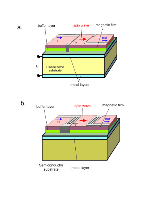
Figure 11: (a). Spin-wave filter on the base of nanosized magnetic film on a piezoelectric substrate. (b). Spin-wave filter with nanosized magnetic film on a semiconductor substrate.

Narrow-band filters can be constructed on the base of periodic antennae (Figure 11b). These antenna structure generate spin waves with the wavevector $q=2\pi/l$, where $l$ is the period of the generating antenna. Filters with periodic antenna structures have more selectivity in comparison with filters with single antennae. The bandwidth of the filter is given by

$$\Delta\omega=\left.\frac{\partial\omega(q)}{\partial q}\right|_{q_{0}}\cdot\frac{2\pi}{lN_{1}N_{2}}$$

where $\omega(q)$ is dispersion relation (19), (20), or (33), $q_{0}=2\pi/l$, $N_{1}$, $N_{2}$ are numbers of periods of generating and receiving antennae, respectively. Thin magnetic film used in the above-mentioned filters must be dielectric and can be garnet, spinel or hexaferrite films. These films can be produced by the laser deposition method or by ion-beam sputtering with following annealing. In [39] band pass spin-wave filters at $5-7$ GHz have been fabricated on the base of submicron thick YIG films produced by the laser deposition on Gd₃Ga₅O₁₂ substrates. In the case, when spin-wave filters are integrated on semiconductor chips, the semiconductor must endure the annealing procedure without any changes for the worse in the semiconductor structure. For this purpose, Si and GaN can be used.

6.2 Field-effect transistors with nanosized magnetic films

As we can see from relations (20), (21) and from figures 4, 5, spin-wave resonance peaks in thin magnetic films have high frequencies and low numbers. For the exchange interaction between layers $I_{d}=$ 0.05-0.1 eV (garnet films, lithium ferrospinel and hexaferrite films [38, 40]) spin-wave resonance frequencies are in Gigahertz and Terahertz frequency bands. Distance between spin-wave resonance peaks is greater in thin films than in thick ones. Since in thin films spin-wave resonances (21) at the given high frequency have lower numbers $n$ and have lower numbers of half-periods of waves on film thickness in comparison with resonances at the same frequency in thick magnetic films, high-frequency resonances in thin films can be exited more easily. This can be used in field-effect transistor (FET) structures. In figure 12 thin dielectric magnetic film is placed under the gate electrode. Applied voltage of the microwave frequency on the gate generates electromagnetic field, which induces spin-wave resonances. In order to increase the magnetic component of the electromagnetic field and to enhance amplitude of resonances, multiferroic layer can be placed between the gate and the magnetic film. The magnetic field of the induced spin-wave resonances interacts with spins of electrons propagating in the channel and modulates the current of the transistor. Consequently, existence of spin-wave resonances in the gate circuit can be regarded as a filter. Choosing the certain spin-wave resonance peak, we can construct FET structure operating in a desirable range of Gigahertz and Terahertz frequency bands.

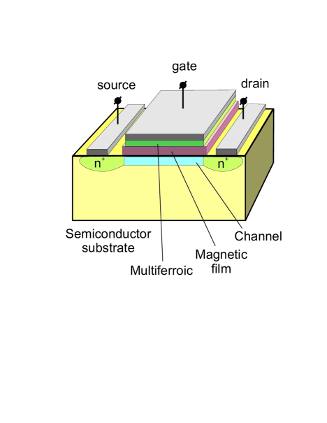
Figure 12: Field-effect transistor with nanosized magnetic film under the gate contact.

7 Conclusions

The results of the investigations can be summarized as follows.

(1) We have studied spin excitations in nanosized magnetic films in the Heisenberg model with magnetic dipole and exchange interactions by the spin operator diagram technique. Dispersion relations of spin waves in two-dimensional magnetic monolayers and in two-layer magnetic films and the spin-wave resonance spectrum in $N$-layer structures are found.

(2) Generalized Landau-Lifshitz equations for thick magnetic films which are derived from first principles, have the integral (pseudodifferential) form, but not differential one with respect to spatial variables. Spin excitations are determined by simultaneous solution of the Landau-Lifshitz equations and the equation for the magnetostatic potential. The use of exchange boundary conditions for solvability of the Landau-Lifshitz equations is incorrect.

(3) The magnetic dipole interaction makes a major contribution to the relaxation of long-wavelength spin waves in thick magnetic films. The spin-wave damping is determined by diagrams in the one-loop approximation, which correspond to three-spin-wave processes. The three-spin-wave processes are accompanied by transitions between thermal excited spin-wave modes. The damping increases directly proportionally to the temperature.

(4) Thin films have a region of low relaxation of long-wavelength spin waves. In thin magnetic films the energy of these waves is less than energy gaps between spin-wave modes, therefore, three-spin-wave processes are forbidden, four-spin-wave processes take place and, as a result of this, the exchange interaction makes a major contribution to the relaxation. It is found that the damping of spin waves propagating in a magnetic monolayer has the form of the quadratic dependence on the temperature and is very low for spin waves with small wavevectors.

(5) Nanosized magnetic films can be used in spin-wave devices. Low damping of long-wavelength spin waves gives us opportunity to construct tunable narrow-band spin-wave filters with high quality at the microwave frequency range. Spin-wave resonances of nanosized magnetic films under gate electrodes in field-effect transistor (FET) structures can be used to construct FET structures operating in Gigahertz and Terahertz frequency bands.

References

- [1] D.D. Stancil, Theory of Magnetostatic Waves (Springer, New York, 1993).
- [2] D.D. Stancil and A. Prabhakar, Spin Waves. Theory and Applications (Springer, New York, 2009).
- [3] P. Kabos and V.S. Stalmachov Magnetostatic Waves and Their Applications (Chapman & Hall, New York, 1994).
- [4] A. Khitun, M. Bao, and K.L.Wang, J. Phys. D: Appl. Phys. 43(26), 264005 (2010).
- [5] B. Lenk, H. Ulrichs, F. Garbs, M. Münzenberg, Physics Reports 507, 107 (2011).
- [6] Sang-Koog Kim, J. Phys. D: Appl. Phys. 43, 264004 (2010).
- [7] Y. Kajiwara, K. Harii, S. Takahashi, J. Ohe, K. Uchida, M. Mizuguchi, H. Umezawa, H. Kawai, K. Ando, K. Takanashi, S. Maekawa, and E. Saitoh, Nature 464, 262 (2010).
- [8] T. Schneider, A.A. Serga, B. Leven, B. Hillebrands, R.L. Stamps, and M.P. Kostylev, Appl. Phys. Lett. 92(2), 022505 (2008).
- [9] Tianyu Liu and G. Vignale, Physical Review Letters 106 (24), 247203 (2011).
- [10] B.A. Kalinikos and A.N. Slavin, J. Phys. C: Solid State Phys. 19(35), 7013 (1986).
- [11] B.A. Kalinikos, M.P. Kostylev, N.V. Kozhus, and A.N. Slavin, J. Phys.: Condens. Matter 2(49), 9861 (1990).
- [12] Linear and Nonlinear Spin Waves in magnetic films and superlattices, Ed. by M.G. Cottam (World Scientific Publishing Co., Singapore, 1994).
- [13] A.G. Gurevich and G.A. Melkov, Magnetization Oscillations and Waves (CRC Press, New York, 1996).
- [14] Yu.A. Izyumov, F.A. Kassan-ogly, and Yu.N. Skryabin, Field Methods in the Theory of Ferromagnetism (Nauka, Moscow, 1974).
- [15] V.G. Vaks, A.I. Larkin, and S.A. Pikin, Sov. Phys.-JETP 53, 281 (1967).
- [16] V.G. Vaks, A.I. Larkin, and S.A. Pikin, Sov. Phys.-JETP 53, 089 (1967).
- [17] L.V. Lutsev, J. Phys.: Condens. Matter 17, 6057 (2005).
- [18] L.V. Lutsev, Mathematical Physics Research Developments, Editor: Morris B. Levy, pp. 141-188 (Nova Science Publishers, New York, 2008).
- [19] R.P. Erickson and D.L. Mills, Phys. Rev. B 43(13), 10715 (1991).
- [20] R.P. Erickson and D.L. Mills, Phys. Rev. B 44(21), 11825 (1991).
- [21] D.L. Mills, Phys. Rev. B 45(22), 13100 (1992).
- [22] R.N. Costa Filho, M.G. Cottam, and G.A. Farias, Solid State Communications 108(7), 439 (1998).
- [23] R.N. Costa Filho, M.G. Cottam, and G.A. Farias, Phys. Rev. B 62(10), 6545 (2000).
- [24] J. Milton Pereira Jr. and R.N. Costa Filho, Eur. Phys. J. B 40, 137 (2004).
- [25] A. Kreisel, F. Sauli, L. Bartosch, and P. Kopietz, Eur. Phys. J. B 71, 59 (2009).
- [26] H.T. Nguyen and M.G. Cottam, J. Phys.: Condens. Matter 23, 126004 (2011).
- [27] E. Meloche, J.I. Mercer, J.P. Whitehead, T. M. Nguyen, and M.L. Plumer, Phys. Rev. B 83(17), 174425 (2011).
- [28] L.V. Lutsev, J. Phys. A: Math. Theor. 40, 11791 (2007).
- [29] A.N. Vasil’ev, Functional Methods in Quantum Field Theory and Statistical Physics (Taylor & Francis Books, New York, 1997).
- [30] T. Matsubara, Prog. Theor. Phys. 14, 351 (1955).
- [31] D.N. Zubarev, Nonequilibrium Statistical Thermodynamics (Plenum, New York, 1974).
- [32] F. Treves, Introduction to Pseudodifferential and Fourier Integral Operators, V.1 (Plenum Press, New York and London, 1982).
- [33] I.V. Rojdestvenski, M.G. Cottam, and A.N. Slavin, Phys. Rev. B 48(17), 12768 (1993).
- [34] S.O. Demokritov,B. Hillebrands, and A.N. Slavin, Physics Reports 348, 441 (2001).
- [35] K.Yu. Guslienko, S.O. Demokritov, B. Hillebrands, and A.N. Slavin, Phys. Rev. B 66(13), 132402 (2002).
- [36] K.Yu. Guslienko and A.N. Slavin, Phys. Rev. B 72(1), 014463 (2005).
- [37] N.Yu. Grigorieva and B.A. Kalinikos, Technical Physics 54(8), 1196 (2009).
- [38] S. Krupička, Physik der Ferrite und der Verwandten Magnetischen Oxide (Academia Verlag der Tschechoslowakischen, Prag, 1973).
- [39] S. A. Manuilov, R. Fors, S. I. Khartsev, and A. M. Grishin, J. Appl. Phys. 105(3), 033917 (2009).
- [40] W.A. Harrison, Electronic Structure and the Properties of Solids. The Physics of the Chemical Bond (W.H. Freeman and Company, San Francisco, 1980).