The Riemann-Hilbert approach to obtain critical asymptotics for Hamiltonian perturbations of hyperbolic and elliptic systems

Abstract

The present paper gives an overview of the recent developments in the description of critical behavior for Hamiltonian perturbations of hyperbolic and elliptic systems of partial differential equations. It was conjectured that this behavior can be described in terms of distinguished Painlevé transcendents, which are universal in the sense that they are, to some extent, independent of the equation and the initial data. We will consider several examples of well-known integrable equations that are expected to show this type of Painlevé behavior near critical points. The Riemann-Hilbert method is a useful tool to obtain rigorous results for such equations. We will explain the main lines of this method and we will discuss the universality conjecture from a Riemann-Hilbert point of view.

1 Introduction

We will discuss the asymptotic behavior of solutions to Hamiltonian perturbations of hyperbolic and elliptic systems of partial differential equations near critical points of the unperturbed system. We will give an overview of recent developments in this area using the Riemann-Hilbert (RH) approach. The systematic study of the critical behavior of such Hamiltonian systems was initiated by Dubrovin and collaborators [17, 18, 19, 20, 21] in a series of papers where it was conjectured that the local behavior of solutions near critical points is to a large extent universal, and that it can be described in terms of distinguished Painlevé transcendents. The conjectured behavior has been proved and verified numerically in various special cases. We will focus mainly on particular cases of Hamiltonian PDEs or systems of PDEs that can be written in a so-called Lax form and that consequently can be solved using the direct and inverse scattering transform, which can be formulated as a RH problem. The Deift/Zhou steepest descent method then provides the tools to obtain asymptotics for the RH problem and for the solution to the system of equations.

Let us first consider the simple quasi-linear hyperbolic equation $u_{t}+6uu_{x}=0$, which is known as the Hopf equation or in-viscid Burgers’ equation. It is a classical fact that solutions to this equation exist only for small times $t>0$ and develop shocks at a certain time. Given initial data $u_{0}(x)$, the solution is given by the method of characteristics in the implicit form

$$u(x,t)=u_{0}(\xi),\qquad x=6tu_{0}(\xi)+\xi.$$ (1.1)

For simplicity, we will only consider smooth initial data that decay sufficiently rapidly at $\pm\infty$. One observes that the derivative of the solution blows up at the critical time

$$t_{c}=\dfrac{1}{\max_{\xi\in\mathbb{R}}[-6u^{\prime}_{0}(\xi)]},$$

see Figure 1. We write $x_{c}$ for the point where the derivative of $u(.,t_{c})$ blows up, and $u_{c}=u(x_{c},t_{c})$.

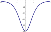
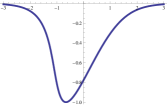
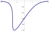
Figure 1: The solution to the Hopf equation with initial data $u_{0}(x)=-{\rm sech}^{2}(x)$ for $t=0$, $t=0.11$, and $t=0.216506$.

The blow-up of the first derivative is called the gradient catastrophe, and we say that $x_{c}$ and $t_{c}$ are the point and time of gradient catastrophe. Locally near $x_{c}$, the solution at the critical time behaves (for generic initial data) like

$$u(x,t_{c})=u_{c}-c(x-x_{c})^{1/3}+{\cal O}(x-x_{c})^{4/3},\qquad\mbox{as $x\to x_{c}$.}$$ (1.2)

In order to avoid the gradient catastrophe, one can perturb the Hopf equation. The Burgers’ equation $u_{t}+6uu_{x}-\epsilon^{2}u_{xx}=0$ is an example of a dissipative regularization, but we will concentrate on dispersive or Hamiltonian perturbations of the Hopf equation. In [17], all Hamiltonian perturbations to the Hopf equation $u_{t}+6uu_{x}=0$ up to order $4$ have been classified, which lead to the class of equations

$$u_{t}+6uu_{x}+\frac{\epsilon^{2}}{24}\left[2cu_{xxx}+4c^{\prime}u_{x}u_{xx}+c^{\prime\prime}u_{x}^{3}\right]+\epsilon^{4}\left[2pu_{xxxxx}\right.\\ \left.+2p^{\prime}(5u_{xx}u_{xxx}+3u_{x}u_{xxxx})+p^{\prime\prime}(7u_{x}u_{xx}^{2}+6u_{x}^{2}u_{xxx})+2p^{\prime\prime\prime}u_{x}^{3}u_{xx}\right]=0,$$ (1.3)

where $p=p(u)$ and $c=c(u)$ are arbitrary smooth functions. For $c=12$, $p=0$, we have the KdV equation

$$u_{t}+6uu_{x}+\epsilon^{2}u_{xxx}=0.$$ (1.4)

For sufficiently smooth initial data $u_{0}(x)=u(x,0,\epsilon)$, solutions to the KdV equation exist for all times $t>0$. For small times, $u$ and its derivatives are bounded and the third derivative term will only contribute up to order ${\cal O}(\epsilon^{2})$ for small $\epsilon$. Near the time and point of gradient catastrophe for the Hopf equation, solutions to KdV start forming oscillations, and the $x$-derivative of the solution is no longer uniformly bounded. The contribution of the dispersive term $\epsilon^{2}u_{xxx}$ in the equation becomes visible in this region: for $t$ slightly bigger than $t_{c}$, it is well-known that there is an interval $[x^{-}(t),x^{+}(t)]$ where the KdV solution $u(x,t,\epsilon)$ shows oscillatory behavior. Outside this interval, the KdV solution can still be approximated by a continuation of the Hopf solution. The oscillations have been studied extensively in many works and are given asymptotically in the small dispersion limit in terms of the solutions to the Whitham equations for KdV and in terms of Jacobi elliptic functions and elliptic integrals [12, 13, 32, 39, 47, 50].

At least before the gradient catastrophe, the small $\epsilon$ behavior for general equations in the family (1.3) is expected to be similar to the behavior for KdV, but few analytical results are available. Even existence of solutions with smooth initial data for small times has not been established in general. For small times, it is not hard to believe that the contributions of the terms of order $\epsilon^{2}$ and $\epsilon^{4}$ will be small. One expects that $u(x,t,\epsilon)=u(x,t)+{\cal O}(\epsilon^{2})$ for $t<t_{c}-\delta$, where $u(x,t)$ is the solution to the Hopf equation with initial data $u_{0}(x)$. It is less obvious what happens for $x$ and $t$ near the point and time of gradient catastrophe. This problem was addressed by Dubrovin in [17], where universality of critical behavior for Hamiltonian perturbations of hyperbolic PDEs was conjectured.

Universality conjecture: the hyperbolic case

It is expected that a generic solution to an equation of the form (1.3) has an expansion of the form

$$u(x,t,\epsilon)=u_{c}+c_{1}\epsilon^{2/7}U(c_{2}\frac{x-x_{c}-c_{3}(t-t_{c})}{\epsilon^{\frac{6}{7}}},c_{4}\frac{t-t_{c}}{\epsilon^{4/7}})+{\cal O}(\epsilon^{4/7}),$$ (1.5)

as $\epsilon\to 0$ and at the same time $x\to x_{c}$ and $t\to t_{c}$ at appropriate speeds, where $x_{c}$ and $t_{c}$ are the point and time of gradient catastrophe. The constants $c_{1},c_{2},c_{3},c_{4}$ depend on the equation and the initial data, but not on $x,t$. The function $U(X,T)$ is expected to be universal, i.e. independent of the equation and independent of the choice of initial data. It should be a solution to the fourth order ODE

$$X=TU-\left(\frac{1}{6}U^{3}+\frac{1}{24}(U_{X}^{2}+2UU_{XX})+\frac{1}{240}U_{XXXX}\right)$$ (1.6)

which is smooth and real for all real values of $X$ and $T$. The existence and uniqueness of such a solution was part of the conjecture, but the existence of a real smooth solution with the asymptotic behavior

$$U(X,T)=\mp(6|X|)^{1/3}+{\cal O}(|X|^{-2/3}),\qquad\mbox{ as $X\to\infty$},$$ (1.7)

for any fixed $T\in\mathbb{R}$, has been proved in [8]. The smoothness of the Painlevé transcendent $U(X,T)$ was already conjectured long time ago for $T=0$ [5, 42], and appeared later to be related to the Gurevich-Pitaevskii special solution to KdV [32, 45, 46]. In the physics literature, $U(X,T)$ shows up in the study of ideal incompressible liquids [37, 38, 29] and in quantum gravity [16]. It appears also in the description of the local eigenvalue behavior in unitary random matrix ensembles with singular edge points [5, 9].

Substituting the asymptotics (1.7) in (1.5) for $t=t_{c}$, we recover (1.2) in the limit $\epsilon\to 0$. Equation (1.6) is known as the second member of the Painlevé I hierarchy and has, given $T\in\mathbb{C}$, solutions that are meromorphic in $X$ with an infinite number of complex poles. The smoothness of $U$ means in other words that no poles lie on the real line. It is remarkable that $U(X,T)$ is an exact solution to the KdV equation written in the form $U_{T}+UU_{X}+\frac{1}{12}U_{XXX}=0$.

Loosely speaking, the conjecture suggests that the local behavior of solutions to Hamiltonian perturbations of the Hopf equation is universally described in terms of $U(X,T)$: the same Painlevé transcendent appears independent of the initial data and independent of the equation. $U$ can be seen as the function which describes the transition between the region where the small dispersion asymptotics are determined by the Hopf equation and the region of oscillatory behavior.

Critical behavior in terms of $U(X,T)$ is expected [18] for more general Hamiltonian perturbations of strictly hyperbolic systems of equations of the form

$$u_{t}+A(u)u_{x}=0,\qquad u=\begin{pmatrix}u_{1}\\ u_{2}\\ \vdots\\ u_{n}\end{pmatrix},$$ (1.8)

where $A(u)$ is a $n\times n$ matrix-valued function of $u$, strict hyperbolicity means that $A$ has real and distinct eigenvalues in the domain of the $(x,t)$-plane under consideration.

In the case of the KdV equation and KdV hierarchy (see below), the universality conjecture has been proved for a class of negative, real analytic initial data $u_{0}(x)$ with one local minimum, and which tend to $0$ rapidly as $x\to\pm\infty$. For the KdV equation, we have (1.5) with the values [6]

$$c_{1}=\frac{2}{(8k)^{2/7}},\quad c_{2}=\frac{1}{(8k)^{1/7}},\quad c_{3}=6u_{c},\quad c_{4}=\frac{12}{(8k)^{3/7}},$$

where $k=-f_{L}^{\prime\prime\prime}(u_{c})$, with $f_{L}$ the inverse of the decreasing part of the initial data $u_{0}$. The expansion holds in a neighborhood of $(x_{c},t_{c})$ which shrinks with $\epsilon$, to be more precise it holds in the double scaling limit where $\epsilon\to 0$, $x\to x_{c}$, $t\to t_{c}$ in such a way that

$$\lim c_{2}\frac{x-x_{c}-c_{3}(t-t_{c})}{\epsilon^{\frac{6}{7}}}=X,\qquad\lim c_{4}\frac{t-t_{c}}{\epsilon^{4/7}}=T,\qquad X,T\in\mathbb{R},$$ (1.9)

Examples

We will now list a number of equations and systems of equations that are expected to belong to the universality class for which $U(X,T)$ describes the solutions locally near the gradient catastrophe.

• The $m$-th time flow of the KdV hierarchy is given by

  $$u_{t}-(-1)^{m}\partial_{x}\mathcal{L}_{m}=0,$$ (1.10)

  where $\mathcal{L}_{m}$ is the Lenard-Magri recursion operator defined by

  $$\partial_{x}\mathcal{L}_{m}=\left(\epsilon^{2}\partial_{x}^{3}+4u\partial_{x}+2u_{x}\right)\mathcal{L}_{m-1},\qquad\mathcal{L}_{0}=u.$$ (1.11)

  For $m=1$, we have the KdV equation, and if we impose $\mathcal{L}_{m}$ to be zero for $u=0$, the second and third equation in the hierarchy are given by

  $$u_{t}-30u^{2}u_{x}-\epsilon^{2}\left(20u_{x}u_{xx}+10uu_{xxx}\right)-\epsilon^{4}u_{xxxxx}=0,$$ (1.12)

  $$u_{t}+140u^{3}u_{x}+\epsilon^{2}\left(70u_{x}^{3}+280uu_{x}u_{xx}+70u^{2}u_{3x}\right)$$

  $$\qquad\qquad\qquad\qquad\qquad\quad+\epsilon^{4}\left(70u_{2x}u_{3x}+42u_{x}u_{4x}+14uu_{5x}\right)+\epsilon^{6}u_{7x}=0,$$ (1.13)

  where we have written $u_{jx}$ for the $j$-th partial derivative of $u$ with respect to $x$. The universality conjecture has been confirmed numerically for the second member of the hierarchy in [22], and an expansion of the form (1.5) was proved analytically in [7] for all equations in the hierarchy.

• For the Camassa-Holm (CH) equation

  $$u_{t}+(3u+2\kappa)u_{x}-\epsilon^{2}\left(u_{xxt}+2u_{x}u_{xx}+uu_{xxx}\right)=0,\qquad t>0,\ x\in\mathbb{R},\ \kappa\in\mathbb{R},$$ (1.14)

  numerical results have been obtained in [30] supporting the universality conjecture, although the equation is not precisely of the form (1.3) or (1.8), see [31].

• The de-focusing nonlinear Schrödinger (NLS) equation

  $$i\epsilon\psi_{t}+\frac{\epsilon^{2}}{2}\psi_{xx}-|\psi|^{2}\psi=0,$$ (1.15)

  can be transformed to the system

  $$\begin{cases}u_{t}+vu_{x}+uv_{x}=0\\ v_{t}+vv_{x}-u_{x}+\frac{\epsilon^{2}}{4}\left(\frac{1}{2}\frac{u_{x}^{2}}{u^{2}}-\frac{u_{xx}}{u}\right)_{x}=0\end{cases},$$ (1.16)

  where $u=-|\psi|^{2}$, $v=\frac{\epsilon}{2i}\left(\frac{\psi_{x}}{\psi}-\frac{\psi_{x}^{*}}{\psi^{*}}\right)$. This is a Hamiltonian perturbation of the system

  $$\begin{pmatrix}u\\ v\end{pmatrix}_{t}+\begin{pmatrix}v&u\\ -1&v\end{pmatrix}\begin{pmatrix}u\\ v\end{pmatrix}_{x}=0,$$ (1.17)

  which is hyperbolic because the eigenvalues of the coefficient matrix are $v\pm\sqrt{-u}$.

• For the Kawahara equation

  $$u_{t}+6uu_{x}+\epsilon^{2}u_{xxx}=\epsilon^{4}u_{xxxxx}$$ (1.18)

  and generalized KdV equations

  $$u_{t}+6u^{n}u_{x}+\epsilon^{2}u_{xxx}=0,$$ (1.19)

  the universality conjecture has been verified numerically in [22].

Universality conjecture: the elliptic case

The focusing nonlinear Schrödinger equation

$$i\epsilon\psi_{t}+\frac{\epsilon^{2}}{2}\psi_{xx}+|\psi|^{2}\psi=0$$ (1.20)

can be seen as a Hamiltonian perturbation of an elliptic system, since it is transformed to the system (1.16) after the substitutions $u=|\psi|^{2}$, $v=\frac{\epsilon}{2i}\left(\frac{\psi_{x}}{\psi}-\frac{\psi_{x}^{*}}{\psi^{*}}\right)$. This is a Hamiltonian perturbation of the system (1.17) which is then of elliptic type since the eigenvalues $v\pm i\sqrt{u}$ are complex conjugate for positive $u$. The Cauchy problem for this equation is ill-posed and the blow-up phenomenon is essentially different than for hyperbolic systems. The system (1.17) can be solved using a hodograph transform method up to a critical time $t_{c}$ where the spatial derivative of $u$ blows up at a point $x_{c}$. This happens when the peak at a local maximum of the solution becomes more and more narrow (or focusses). This critical point is called a point of elliptic umbilic catastrophe, and a conjecture has been formulated in [21] concerning the local behavior of the NLS equation near this point. The key role in this conjecture is played by the Boutroux tritronquée solution to the first Painlevé equation

$$Q_{ZZ}=Z+6Q^{2},$$ (1.21)

characterized by the asymptotic behavior

$$Q(Z)\sim-\sqrt{\frac{Z}{6}},\qquad\mbox{ as $Z\to\pm\infty$ in the sector $|\arg Z|<\frac{4\pi}{5}$.}$$ (1.22)

It is known that this is a meromorphic function with infinitely many poles in the sector of the complex plane where $|\arg Z|\geq\frac{4\pi}{5}$. In the complementary sector $|\arg Z|<\frac{4\pi}{5}$, $Q$ has no poles for sufficiently large $Z$ (this would contradict the asymptotic behavior (1.22)) and no poles at all on the positive half-line [33], but this does not exclude the possibility that a finite number of poles is present in this sector. It was conjectured by Dubrovin, Grava, and Klein in [21] that $Q$ has no poles at all in the sector $|\arg Z|<\frac{4\pi}{5}$. The second part of the conjecture, in analogy to the hyperbolic case, describes the behavior of the solution to the focusing NLS equation: it is expected to have an asymptotic expansion where the first error term to the unperturbed solution is of order $\epsilon^{2/5}$ and can be described completely in terms of the tritronquée solution $Q(Z)$ evaluated at complex arguments $Z$.

Substantial progress has been made on a proof of the second part of the conjecture in the recent work [2], we will comment in more detail on this later on. The poles of $Q$ have been studied in [40], but the first part of the conjecture is still open. It was discussed in [18] that an expansion in terms of $Q(Z)$ is not exclusively expected for the focusing NLS equation, but also for more general Hamiltonian perturbations of elliptic systems. The tritronquée solution $Q$ is also relevant for the asymptotics of recurrence coefficients of certain orthogonal polynomials on a complex contour [23, 25].

Outline

We will not discuss classification results or try to formulate the most general form of the conjectures, for these topics we refer to [17, 18, 19, 20, 21, 22]. Rather we want to focus on techniques that can be used to prove the universality conjectures in various special cases. The best one can do so far is to try to prove the universality conjectures for systems of equations that can be solved using the inverse scattering transform. Then one can formulate a RH problem which characterizes solutions to the system of equations, and an asymptotic analysis of this RH problem can in principle lead to the critical asymptotics in terms of the Painlevé transcendents $U$ and $Q$, which themselves can be characterized in terms of a so-called model RH problem. Without going into the technical details, we will give an overview of this method in the case of the KdV equation (following [12, 13, 6]), and indicate the differences for the KdV hierarchy (following [7]). Afterwards we will recall the RH problems associated to the Camassa-Holm equation [4] and the de-focusing and focusing NLS equation [44], and explain the main lines of the procedure that can be followed to obtain asymptotics for solutions of those equations. We will also give heuristic arguments supporting the universal nature of the critical behavior from the Riemann-Hilbert point of view.

2 RH problems for Painlevé transcendents

The Painlevé transcendents $U$ and $Q$, which are the central objects in the universality conjectures, can be characterized in terms of RH problems. We will state the RH problems here, and we will explain that the absence of poles is equivalent to the solvability of the RH problems.

2.1 RH problem for $P_{I}^{2}$ solution $U$

The function $U(X,T)$ is characterized by the following RH problem.

RH problem for $\Psi$:

• $\Psi=\Psi(\zeta;X,T)$ is analytic for $\zeta\in\mathbb{C}\setminus\Gamma$, with $\Gamma=\mathbb{R}\cup e^{\frac{6\pi i}{7}}\mathbb{R}^{+}\cup e^{-\frac{6\pi i}{7}}\mathbb{R}^{+}$ oriented as in Figure 2.

• $\Psi$ has continuous boundary values $\Psi_{\pm}$ ($+$ referring to the left side of the contour, $-$ to the right side according to the orientation in Figure 2) on $\Gamma\setminus\{0\}$, and we have

  $$\Psi_{+}(\zeta)=\Psi_{-}(\zeta)\begin{pmatrix}0&1\\ -1&0\end{pmatrix}, \zeta\in\mathbb{R}^{-}$$ for , (2.1)

  $$\Psi_{+}(\zeta)=\Psi_{-}(\zeta)\begin{pmatrix}1&1\\ 0&1\end{pmatrix}, \zeta\in\mathbb{R}^{+}$$ for , (2.2)

  $$\Psi_{+}(\zeta)=\Psi_{-}(\zeta)\begin{pmatrix}1&0\\ 1&1\end{pmatrix}, \zeta\in e^{\pm\frac{6\pi i}{7}}\mathbb{R}^{+}$$ for . (2.3)

• $\Psi$ has the following behavior at infinity,

  $$\Psi(\zeta)=\left(I+\frac{A_{1}(X,T)}{\zeta}+{\cal O}(\zeta^{-2})\right)\zeta^{-\frac{1}{4}\sigma_{3}}Ne^{-\theta(\zeta;X,T)\sigma_{3}},$$ (2.4)

  where $\sigma_{3}=\begin{pmatrix}1&0\\ 0&-1\end{pmatrix}$, and $N$ and $\theta$ are given by

  $$N=\frac{1}{\sqrt{2}}\begin{pmatrix}1&1\\ -1&1\end{pmatrix}e^{-\frac{\pi i}{4}\sigma_{3}},\qquad\theta(\zeta;X,T)=\frac{1}{105}\zeta^{7/2}-\frac{T}{3}\zeta^{3/2}+X\zeta^{1/2},$$ (2.5)

  and where $A_{1}(X,T)$ is a matrix independent of $\zeta$.

Figure 2: The jump contour $\Gamma$ and the jump matrices for $\Psi$

It was proved in [8] that this RH problem has a solution for all real values of $X,T$, and that the function

$$U(X,T)=2A_{1,11}(X,T)-A_{1,12}^{2}(X,T)$$ (2.6)

is a real pole-free solution to equation (1.6) which has the asymptotic behavior (1.7). General solutions to (1.6) are characterized by a similar RH problem, but with jumps also on the four rays $e^{\pm\frac{2\pi i}{7}}\mathbb{R}^{+}$ and $e^{\pm\frac{4\pi i}{7}}\mathbb{R}^{+}$ [34]. The jump matrices are all triangular with ones on the diagonal, and the triangular structure is as follows: the jump matrices are upper-triangular on $\mathbb{R}$, $e^{\pm\frac{4\pi i}{7}}\mathbb{R}^{+}$, and lower-triangular on $e^{\pm\frac{2\pi i}{7}}\mathbb{R}^{+}$ and $e^{\pm\frac{6\pi i}{7}}\mathbb{R}^{+}$. The off-diagonal entries of the jump matrices are called Stokes multipliers and satisfy certain constraints. Given $T\in\mathbb{C}$, there is a one-to-one correspondence between the set of admissible Stokes multipliers (also called the monodromy surface) and the solutions of the $P_{I}^{2}$ equation. The RH problem is known to be solvable if and only if the corresponding Painlevé solution is analytic at the value $(X,T)$, or in other words the RH problem is not solvable if and only if $(X,T)$ is a pole of the corresponding Painlevé solution.

2.2 RH problem for PI

The Boutroux tritronquée solution $Q(Z)$ of the Painlevé I equation is characterized by another RH problem.

RH problem for $\Phi$:

• $\Phi=\Phi(\zeta;Z)$ is analytic for $\zeta\in\mathbb{C}\setminus\Gamma^{\prime}$, with $\Gamma^{\prime}=\mathbb{R}\cup e^{\frac{2\pi i}{5}}\mathbb{R}^{+}\cup e^{-\frac{2\pi i}{5}}\mathbb{R}^{+}$ oriented as in Figure 3.

• $\Phi$ satisfies the following jump relations on $\Gamma^{\prime}\setminus\{0\}$,

  $$\Phi_{+}(\zeta)=\Phi_{-}(\zeta)\begin{pmatrix}0&i\\ i&0\end{pmatrix}, \zeta\in\mathbb{R}^{-}$$ for , (2.7)

  $$\Phi_{+}(\zeta)=\Phi_{-}(\zeta)\begin{pmatrix}1&0\\ i&1\end{pmatrix}, \zeta\in\mathbb{R}^{+}$$ for , (2.8)

  $$\Phi_{+}(\zeta)=\Phi_{-}(\zeta)\begin{pmatrix}1&i\\ 0&1\end{pmatrix}, \zeta\in e^{\pm i\frac{2\pi}{5}}\mathbb{R}^{+}$$ for . (2.9)

• $\Phi$ has the following behavior at infinity,

  $$\Phi(\zeta)=\left(I+\frac{B_{1}(Z)}{\zeta}+{\cal O}(\zeta^{-2})\right)\zeta^{-\frac{1}{4}\sigma_{3}}\frac{1}{\sqrt{2}}\begin{pmatrix}1&1\\ 1&-1\end{pmatrix}e^{-\tilde{\alpha}(\zeta;Z)\sigma_{3}},$$ (2.10)

  where $\tilde{\alpha}$ is given by

  $$\tilde{\alpha}(\zeta;Z)=\frac{4}{5}\zeta^{5/2}-Z\zeta^{1/2}.$$ (2.11)

Figure 3: The jump contour $\Gamma^{\prime}$ and the jump matrices for $\Phi$

The function

$$Q(Z)=B_{1,21}^{2}-2B_{1,22}$$ (2.12)

is the tritronquée solution to Painlevé I [35], and given $Z\in\mathbb{C}$, the RH problem for $\Phi$ is solvable if and only if $Z$ is not a pole of $Q$. A general solution to the Painlevé I equation can be obtained in terms of a RH problem with triangular jumps on the contour $\mathbb{R}\cup e^{\pm i\frac{2\pi}{5}}\mathbb{R}^{+}\cup e^{\pm i\frac{4\pi}{5}}\mathbb{R}^{+}$ [35, 24].

In order to discuss the solvability of this RH problem, let us first introduce the homogeneous RH problem for $\Phi$: we say that $\Phi_{0}$ is a solution to the homogeneous RH problem if it satisfies conditions (a) and (b) of the RH problem for $\Phi$, and it has the asymptotic behavior

$$\Phi_{0}(\zeta)={\cal O}(\zeta^{-3/4})e^{-\tilde{\alpha}(\zeta;Z)\sigma_{3}},\qquad\mbox{ as $\zeta\to\infty$.}$$ (2.13)

Following the vanishing lemma procedure [24, 26, 27], the solvability of the RH problem for $\Phi$ is equivalent to the fact that the homogeneous version of the RH problem has only the trivial zero solution: the RH problem for $\Phi$ with parameter $Z\in\mathbb{C}$ is solvable if and only if the homogeneous RH problem has only the vanishing solution $\Phi_{0}\equiv 0$. To prove this, one can follow the procedure developed in [10, 26, 27] (which works for a fairly general class of RH problems) and show that a certain singular integral operator related to the RH problem is a Fredholm operator of index zero.

So in order to have smoothness of $Q$ for $|\arg Z|<\frac{4\pi}{5}$, it suffices to show that the homogeneous RH problem has only the zero solution (such a result is called a vanishing lemma) for $|\arg Z|<\frac{4\pi}{5}$. Then the RH problem for $\Phi$ is solvable, and $Q$ has no pole at $Z$.

A vanishing lemma has been proved for the $P_{I}^{2}$ RH problem for real $X$ and $T$ [8], but this turns out to be considerably more complicated in the PI case, even for positive real values of $Z$.

3 Small dispersion asymptotics for solutions to KdV: the Riemann-Hilbert approach

We will now give an overview of the RH method to obtain asymptotics for solutions to the KdV equation in the small dispersion limit. The method consists of three steps: first one has to construct a RH problem that characterizes solutions to the KdV equation. This can be done using scattering theory for the Schrödinger operator. The jump matrices in the RH problem will depend on the initial data via a reflection coefficient. The second step requires asymptotic information about the reflection coefficient as $\epsilon\to 0$. Such results were obtained in [43] using WKB techniques. Once this information is gathered, one can start with the final step which is the asymptotic analysis of the RH problem using the Deift/Zhou steepest descent method [14].

3.1 Construction of a RH problem related to the Schrödinger operator

The key observation here is that the KdV equation can be written in the Lax form $L_{t}=[L,A]$, where $L$ is the Schrödinger operator, and $A$ is an antisymmetric operator:

$$Lf=\epsilon^{2}\partial_{x}^{2}f+uf,\qquad Af=A=4\epsilon^{2}\partial_{x}^{3}f+3\left(u\partial_{x}f+\partial_{x}(uf)\right).$$ (3.1)

We consider potentials $u(x)$ that are smooth and decay sufficiently fast at $\pm\infty$. For a general real potential $u(x)$, $L$ has a finite number of purely imaginary eigenvalues $\lambda_{j}$ for which the linear Schrödinger equation $Lf=\lambda f$ has solutions decaying both at $+\infty$ and at $-\infty$. For $\lambda<0$, it admits solutions $\psi_{\pm}$ and $\phi_{\pm}$ satisfying the oscillatory asymptotic conditions

$$\lim_{x\to+\infty}\psi_{\pm}(\lambda;x,t,\epsilon)e^{\pm\frac{i}{\epsilon}\sqrt{-\lambda}x}=1,$$ (3.2)

$$\lim_{x\to-\infty}\phi_{\pm}(\lambda;x,t,\epsilon)^{\mp\frac{i}{\epsilon}\sqrt{-\lambda}x}=1.$$ (3.3)

Those solutions are called Jost solutions. They are related by a connection matrix given by

$$\begin{pmatrix}\psi_{+}(\lambda)&\psi_{-}(\lambda)\end{pmatrix}=\begin{pmatrix}\phi_{-}(\lambda)&\phi_{+}(\lambda)\end{pmatrix}\begin{pmatrix}a(\lambda;t,\epsilon)&\overline{b}(\lambda;t,\epsilon)\\ b(\lambda;t,\epsilon)&\overline{a}(\lambda;t,\epsilon)\end{pmatrix},\qquad\lambda<0.$$ (3.4)

The ratio $r(\lambda;t,\epsilon)=\frac{b}{a}(\lambda;t,\epsilon)$ is called the reflection coefficient for the Schrödinger equation.

It is well-known that $\psi_{+}$ ($\psi_{-}$) and $\phi_{+}$ ($\phi_{-}$) can be extended analytically to the upper (lower) half plane. The vector-valued function

$$M(\lambda;x,t,\epsilon)=\begin{cases}\begin{pmatrix}\phi_{+}&\frac{1}{a}\psi_{+}\end{pmatrix}e^{\frac{-i}{\epsilon}x(-\lambda)^{1/2}\sigma_{3}},&\mbox{ as $\lambda\in\mathbb{C}^{+}$},\\[12.91663pt] \begin{pmatrix}\frac{1}{a^{*}}\psi_{-}&\phi_{-}\end{pmatrix}e^{\frac{-i}{\epsilon}x(-\lambda)^{1/2}\sigma_{3}},&\mbox{ as $\lambda\in\mathbb{C}^{-}$},\end{cases}$$ (3.5)

is meromorphic in $\mathbb{C}\setminus R$ and it can be showed using (3.4) and asymptotic properties of the Jost solutions that $M$ satisfies the following RH conditions [44, 11, 12, 6]

RH problem for $M$

• $M(\lambda;x,t,\epsilon)$ is meromorphic for $\lambda\in\mathbb{C}\backslash\mathbb{R}$,

• $M$ has continuous boundary values $M_{\pm}(\lambda)$ for $\lambda\in\mathbb{R}\setminus\{0\}$ that satisfy the jump conditions

  $$M_{+}(\lambda)=M_{-}(\lambda){\small\begin{pmatrix}1&r(\lambda;t,\epsilon)e^{\frac{2i}{\epsilon}x(-\lambda)^{1/2}}\\ -\bar{r}(\lambda;t,\epsilon)e^{\frac{-2i}{\epsilon}x(-\lambda)^{1/2}}&1-|r(\lambda;t,\epsilon)|^{2}\end{pmatrix}} \lambda<0$$ for , (3.6)

  $$M_{+}(\lambda)=M_{-}(\lambda)\sigma_{1},\quad\sigma_{1}=\begin{pmatrix}0&1\\ 1&0\end{pmatrix} \mbox{ for $\lambda>0$}.$$ (3.7)

• As $\lambda\to\infty$, we have $M(\lambda;x,t,\epsilon)\to\begin{pmatrix}1&1\end{pmatrix}$.

The potential $u(x,t,\epsilon)$ can then be recovered from the equation

$$u(x,t,\epsilon)=-2i\epsilon\lim_{\lambda\to\infty}\sqrt{-\lambda}\partial_{x}(M_{11}(\lambda;x,t,\epsilon)-1).$$ (3.8)

In general $M$ has a finite number of simple poles on the imaginary axis, which are the eigenvalues of the Schrödinger operator. One has to impose additional conditions on the residues of $M$ to have a unique RH solution. If the potential $u(x)$ is negative, the Schrödinger equation has no point spectrum and $M$ is holomorphic in $\mathbb{C}\setminus\mathbb{R}$. Then one can also use the $x$-derivatives of the Jost solutions to construct the second row of a $2\times 2$ matrix $M$ satisfying the same jump condition, and the asymptotic condition

$$M(\lambda)\sim\begin{pmatrix}1&1\\ i\sqrt{-\lambda}&-i\sqrt{-\lambda}\end{pmatrix},\qquad\mbox{ as $\lambda\to\infty$.}$$ (3.9)

A matrix RH problem is for several reasons more convenient to work with than a vector RH problem.

The above construction works for any potential $u(x)$ decaying sufficiently fast at $\pm\infty$, it is not necessary that $u=u(x,t,\epsilon)$ solves the KdV equation. However, for general potentials $u(x,t,\epsilon)$, the time-dependence of $r$ is not explicitly given. On the other hand if $u(x,t,\epsilon)$ satisfies a suitable Lax type equation $L_{t}=[L,A]$, the time evolution of $r$ can be explicitly calculated, and the eigenvalues $\lambda_{j}$ are independent of $t$. In the KdV case, one has [28]

$$r(\lambda;t,\epsilon)=r_{0}(\lambda;\epsilon)e^{\frac{8i}{\epsilon}t(-\lambda)^{\frac{3}{2}}}.$$ (3.10)

This is a crucial observation: if we know the initial reflection coefficient corresponding to the initial data $u_{0}(x)$ (the direct scattering transform), then we know the reflection coefficient at any time $t>0$. In order to find the solution $u(x,t,\epsilon)$ at time $t>0$, it suffices to solve the RH problem for $M$ at time $t>0$ (the inverse scattering transform).

3.2 Semi-classical asymptotics for the reflection coefficient

The solution to the Cauchy problem for KdV is characterized in terms of the RH problem for $M$. The jump matrix for $M$ depends on the reflection coefficient $r_{0}$, which depends in a simple explicit way on $t$, but in a much more complicated way on the spectral variable $\lambda$ and on $\epsilon$. Since we are interested in the small $\epsilon$ behavior of the RH solution $M$, inevitably we need small $\epsilon$ asymptotics for the initial reflection coefficient $r_{0}$. Detailed asymptotics were obtained in [43] for negative initial data with a single negative hump that are analytic in a sufficiently large neighborhood of the real line, and we will concentrate on such data in what follows. For $\lambda<-1$, $r_{0}(\lambda;\epsilon)$ decays rapidly as $\epsilon\to 0$, and for $-1<\lambda<0$, it is oscillatory and has the leading order behavior

$$r_{0}(\lambda;\epsilon)\sim i\exp\left(-\frac{2i}{\epsilon}\rho(\lambda)\right),\qquad\mbox{ as $\epsilon\to 0$},$$ (3.11)

where $\rho(\lambda)=\frac{1}{2}\int_{\lambda}^{0}\frac{f_{L}(\xi)}{\sqrt{\xi-\lambda}}d\xi$, and $f_{L}$ is the inverse of the decreasing part of the initial data $u_{0}$. Near $-1$, there is a subtle transition between the decay and oscillatory behavior.

Substituting $r_{0}$ in the jump matrix of the RH problem by its leading order asymptotics (3.11), we obtain the jump relation $M_{+}(\lambda)=M_{-}(\lambda)v_{M}(\lambda)$ for $\lambda\in\mathbb{R}$, with

$$v_{M}(\lambda)\sim I \lambda<-1$$ for , (3.12)

$$v_{M}(\lambda)\sim{\small\begin{pmatrix}1&i\exp\left(-\frac{2i}{\epsilon}(\rho(\lambda)-\alpha(\lambda))\right)\\ i\exp\left(\frac{2i}{\epsilon}(\rho(\lambda)-\alpha(\lambda))\right)&0\end{pmatrix}} -1<\lambda<0$$ for , (3.13)

$$v_{M}(\lambda)=\sigma_{1} \mbox{ for $\lambda>0$},$$ (3.14)

where $\alpha(\lambda)=x(-\lambda)^{1/2}+4t(-\lambda)^{3/2}$. It is not obvious at all that one can proceed with the RH analysis, neglecting the corrections to the leading order behavior of the reflection coefficient. This needs to be justified, and especially for $\lambda$ near $-1$, technical issues need to be handled. We will not address this here, since it is our goal to give a flavour of the method only, we refer the reader to [6, 7] for details.

3.3 Steepest descent analysis of the RH problem

The Deift/Zhou steepest descent method was developed in [14] and applied to the small dispersion limit for the KdV equation in [12, 13]. The method consists of a number of invertible transformations of the RH problem, and the goal of this series of transformations is to obtain a RH problem for which the jump matrices are uniformly close to the identity matrix as $\epsilon\to 0$ (or in a more complicated double scaling limit where $x\to x_{c}$, $t\to t_{c}$ simultaneously with $\epsilon\to 0$), and with a solution that tends to $I$ as $\lambda\to\infty$. For such RH problems, one can apply small norm theory to prove that the solution is uniformly close to the identity matrix for small $\epsilon$ and to obtain the next terms in the asymptotic series of the solution. Inverting each of the transformations, one obtains asymptotics for $M$ from the asymptotics for the final small norm RH solution.

The first transformation requires the construction of a $g$-function, which has suitable jump conditions and asymptotic behavior. For $x,t$ sufficiently close to $x_{c},t_{c}$, the $g$-function $g=g(\lambda;x,t)$ is defined by the scalar RH conditions

• $g$ is analytic in $\mathbb{C}\setminus[u,+\infty)$,

• $g$ has the jump relations

  $$g_{+}(\lambda)+g_{-}(\lambda)=0, \lambda\in(0,+\infty)$$ for , (3.15)

  $$g_{+}(\lambda)+g_{-}(\lambda)-2\rho(\lambda)+2\alpha(\lambda)=0, \mbox{ for $\lambda\in(u,0)$},$$ (3.16)

• $g(\lambda)={\cal O}(\lambda^{-1/2})$ as $\lambda\to\infty$.

Given $u$, this scalar RH problem has a solution (which is unique if one imposes suitable behavior of $g$ near $u$ and $0$) that can be expressed explicitly as an integral transform of the inverse of the initial data. In order to analyze the KdV solution in the vicinity of $x_{c}$ and $t_{c}$, the choice of the point $u$ is crucial: it has to be chosen as $u=u_{c}=u(x_{c},t_{c})$.

The $g$-function is an essential ingredient for the asymptotic analysis of the RH problem for $M$. It clears the road for a transformation of the RH problem to one with jump conditions of the following form, on a jump contour as the one shown in Figure 4:

RH problem for $S$

• $S$ is analytic in $\mathbb{C}\setminus\Sigma_{S}$,

• $S_{+}(\lambda)=S_{-}(\lambda)v_{S}$ for $\lambda\in\Sigma_{S}$, and as $\epsilon\to 0$, the jump matrix $v_{S}$ has the leading order behavior

  $$v_{S}(\lambda)\sim\begin{cases}\begin{array}[]{lr}\begin{pmatrix}1&ie^{\frac{2i}{\epsilon}\phi(\lambda)}\\ 0&1\end{pmatrix},&\mbox{ on $\Sigma_{1}$},\\[12.91663pt] \begin{pmatrix}1&0\\ ie^{-\frac{2i}{\epsilon}\phi(\lambda)}&1\end{pmatrix},&\mbox{ on $\Sigma_{2}$,}\\[12.91663pt] \begin{pmatrix}e^{-\frac{2i}{\epsilon}\phi_{+}(\lambda)}&i\\ i&0\end{pmatrix},&\mbox{ as $\lambda\in(u_{c},0)$,}\\[12.91663pt] I,&\mbox{ as $\lambda\in(-\infty,-1-\delta_{1})\cup(0,+\infty)$.}\end{array}\end{cases}$$ (3.17)

• $S(\lambda)=\left(I+{\cal O}(\lambda^{-1})\right)\begin{pmatrix}1&1\\ i\sqrt{-\lambda}&-i\sqrt{-\lambda}\end{pmatrix}$ as $\lambda\to\infty$.

The function $\phi$ appearing in the jump matrices is given by

$$\phi(\lambda)=g(\lambda)-\rho(\lambda)+\alpha(\lambda),$$ (3.18)

and vanishes at the point $\lambda=u_{c}$. It can be expressed explicitly as

$$\phi(\lambda;x,t)=-\sqrt{u_{c}-\lambda}F(u_{c};x,t)+\dfrac{2}{3}(u_{c}-\lambda)^{\frac{3}{2}}F^{\prime}(u_{c};x,t)\\ -\dfrac{4}{15}(u_{c}-\lambda)^{\frac{5}{2}}F^{\prime\prime}(u_{c};x,t)-\dfrac{4}{15}\int_{u_{c}}^{\lambda}F^{\prime\prime\prime}(\xi;x,t)(\xi-\lambda)^{\frac{5}{2}}d\xi,$$ (3.19)

where $F(\lambda;x,t)=-x+6\lambda t+f_{L}(\lambda)$.

Figure 4: The jump contour $\Sigma_{S}$ and the jumps for $S$ in the limit $\epsilon\to 0$

The sign of the real part of $\phi$ is such that the exponentials in the jump matrices decay uniformly as $\epsilon\to 0$ on the jump contour, except in the vicinity of $u_{c}$, where $\phi$ behaves like

$$\phi(\lambda;x_{c},t_{c})=-c(u_{c}-\lambda)^{7/2}(1+{\cal O}(\lambda-u_{c})),\qquad\mbox{ as $\lambda\to u_{c}$.}$$ (3.20)

The constant $c$ is strictly positive whenever the generic condition $f_{L}^{\prime\prime\prime}(u_{c})\neq 0$ holds.

Global parametrix

Ignoring a small neighborhood of $u_{c}$ and the corrections to the leading order behavior as $\epsilon\to 0$, one arrives at a RH problem with jump only on $(u_{c},+\infty)$: the jump on $(u_{c},0)$ is $i\sigma_{1}$ and the jump on $(0,+\infty)$ is $\sigma_{1}$, where $\sigma_{1}=\begin{pmatrix}0&1\\ 1&0\end{pmatrix}$. This RH problem can be solved explicitly, indeed the function

$$P^{(\infty)}(\lambda)=(-\lambda)^{1/4}(u_{c}-\lambda)^{-\sigma_{3}/4}\begin{pmatrix}1&1\\ i&-i\end{pmatrix}$$ (3.21)

satisfies the required jump relations and as $\lambda\to\infty$, it behaves as prescribed by condition (c) in the RH problem for $S$.

Local parametrix

Since we have neglected a neighborhood of $u_{c}$ so far, where the jump matrix $v_{S}$ is not uniformly close to the identity matrix, it is necessary to construct a local parametrix in the vicinity of $u_{c}$, which satisfies approximately the same jump conditions than $S$, and which ’matches’ in an appropriate way with the global parametrix. This construction is rather technical but the parametrix can be constructed explicitly in terms of $\Psi$, the solution to the $P_{I}^{2}$ RH problem discussed in Section 2.1. It appears that this is true independently of the precise form of the function $\phi$. Only the local behavior of $\phi$ near $u_{c}$ matters: whenever $\phi(\lambda)\sim-c(u_{c}-\lambda)^{7/2}$ with $c>0$ as $\lambda\to u_{c}$, the local parametrix can be constructed in terms of $\Psi$. The power of vanishing $7/2$ can be identified with the power $7/2$ in the asymptotic behavior for $\Psi$ in (2.4) and (2.5). This is a first indication that the $P_{I}^{2}$ solution $U(X,T)$ plays a role in much more general settings. Indeed if we would consider the RH problem for $M$, but with more complicated time-dependence of the reflection coefficient (for example corresponding to another equation than KdV), the local parametrix would still be built out of $\Psi$. This supports, from the RH point of view, the conjecture that $U(X,T)$ is in some sense universal.

Remark 3.1

If one wants to perform an asymptotic analysis of the RH problem for $M$ away from the critical point $(x_{c},t_{c})$ as in [12] (for example for $t<t_{c}$), the main difference is that $\phi(\lambda)\sim-c(u-\lambda)^{3/2}$, so $\phi$ vanishes at a slower rate. The local parametrix can in this case be constructed in terms of the Airy function.

Asymptotics for $M$

Multiplying $S$ by the inverse of the local parametrix near $u_{c}$ and by the inverse of the global parametrix elsewhere, one obtains a function $R$ which solves a so-called small-norm RH problem: one can show that $R$ tends to the identity matrix in the double scaling limit where $\epsilon\to 0$, $x\to x_{c}$, $t\to t_{c}$ at appropriate speeds. One can even obtain the next terms in the asymptotic series for $R$, which are of order $\epsilon^{1/7}$ and order $\epsilon^{2/7}$, and which can be expressed explicitly in terms of $U(X,T)$. Inverting the transformations $S\mapsto R$, $T\mapsto S$, and $M\mapsto T$, this produces an asymptotic expansion for $M$ and, by (3.8), for the KdV solution $u$. In particular the method described here allows one to prove that the KdV solution has an expansion of the form (1.5).

Remark 3.2

The above RH analysis works fine for initial data that are such that the initial reflection coefficient is analytic and decays sufficiently fast at infinity. If the initial reflection coefficient would be $C^{1}$ or $C^{2}$ instead of analytic, the usual RH techniques cannot be applied, but one may hope that recently developed dbar techniques [15, 41] could help to get around this problem.

4 The Riemann-Hilbert approach for other equations

4.1 The KdV hierarchy

The equations in the KdV hierarchy can be written as a Lax equation

$$L_{t}=[L,A_{m}],$$ (4.1)

where $L$ is (as for the KdV equation) the Schrödinger operator $L=\epsilon^{2}\partial_{x}^{2}+u$ and where $A_{m}$ is an antisymmetric higher order operator with leading order $(-1)^{m+1}4^{m}\epsilon^{2m}\partial_{x}^{2m+1}$. The lower order terms of $A_{m}$ are determined by the requirement that $[L,A_{m}]$ is an operator of multiplication with a function depending on $u,u_{x},\ldots,u_{(2m+1)x}$. For $m=1$, the operator $A$ was given in (3.1). As explained in Section 3.1, the Jost solutions to the Schrödinger equation can be used to construct a RH problem. The only difference here is the time evolution of the reflection coefficient, which is now given by

$$r(\lambda;t,\epsilon)=r_{0}(\lambda;\epsilon)e^{\frac{2.4^{m}i}{\epsilon}t(-\lambda)^{\frac{2m+1}{2}}}.$$ (4.2)

With this modification, the RH problem for $M$ given in Section 3.1 still characterizes the solution to the Cauchy problem for the $m$-th equation in the KdV hierarchy which is given by (3.8). In the asymptotic analysis of the RH problem, the $g$-function has to be modified and the function $\phi$ will be somewhat different, but the main issue is that it will still behave like in (3.20) locally near $u_{c}$. Details can be found in [7].

4.2 The Camassa-Holm equation

The Camassa-Holm equation (1.14) is the compatibility condition of the Lax equations

$$\epsilon^{2}f_{xx}=\left(\frac{1}{4}-\lambda(u-\epsilon^{2}u_{xx}+\kappa)\right)f$$ (4.3)

$$f_{t}=-\left(\frac{1}{2\lambda}+u\right)f_{x}+\frac{u_{x}}{2}f.$$ (4.4)

This fact has been used in [4] to construct a RH problem that characterizes solutions to the Camassa-Holm equation. The RH solution is, in a somewhat similar manner as for the KdV problem, constructed using fundamental solutions to the spatial Lax equation (4.3), and the jump matrix contains a reflection coefficient for this equation. Equation (4.3) is related to the Schrödinger equation through the unitary Liouville transform [3]. We present the RH problem in the variable $z$, where $z^{2}=-\lambda$.

RH problem for $M^{CH}$

• $M^{CH}:\mathbb{C}\setminus\mathbb{R}\to\mathbb{C}^{1\times 2}$ is meromorphic for $z\in\mathbb{C}\backslash\mathbb{R}$,

• $M^{CH}$ has continuous boundary conditions $M_{\pm}(\lambda)$ for $z\in\mathbb{R}$ that satisfy the jump conditions

  $$M_{+}^{CH}(z)=M_{-}^{CH}(z){\small\begin{pmatrix}1-|r(z;t,\epsilon)|^{2}&r(z;t,\epsilon)e^{-2iyz}\\ -\bar{r}(z;t,\epsilon)e^{2izy}&1\end{pmatrix}}\qquad\mbox{ for $z\in\mathbb{R}$,}$$ (4.5)

• as $z\to\infty$, we have

  $$M^{CH}(z)=\begin{pmatrix}1&1\end{pmatrix}+o(1).$$ (4.6)

Again, in general there is a finite number of poles where one has to add residue conditions to ensure the uniqueness of a RH solution. In the simplest case there are no eigenvalues and $M^{CH}=M^{CH}(z;y,t,\epsilon)$ is holomorphic in $\mathbb{C}\setminus\mathbb{R}$.

The CH solution $u(x,t,\epsilon)$ is recovered from the relation

$$u(x,t,\epsilon)=\left.\frac{\partial}{\partial t}\ln\frac{M_{1}^{CH}}{M_{2}^{CH}}(\frac{i}{2};y,t,\epsilon)\right|_{y=y(x,t)},$$ (4.7)

where $y(x,t)$ is given by

$$x=y+\ln\frac{M_{1}^{CH}}{M_{2}^{CH}}(\frac{i}{2};y,t,\epsilon).$$

The time evolution for the reflection coefficient is explicitly given:

$$r(z;t,\epsilon)=r_{0}(z;\epsilon)\exp\left(\frac{4itz}{\epsilon}\frac{1}{1+4z^{2}}\right).$$ (4.8)

This RH problem has been used to obtain large time asymptotics for CH solutions [3, 4]. In the small dispersion setting, there is an additional complication because the reflection coefficient depends in a nontrivial way on the small parameter $\epsilon$. If one makes the ansatz that the initial reflection coefficient is analytic in $z$ and behaves like

$$r_{0}(z;\epsilon)\sim i\exp\left(-\frac{2i}{\epsilon}\rho(z)\right),\qquad\mbox{ as $\epsilon\to 0$}$$ (4.9)

for a suitable function $\rho$, one could proceed in a similar manner as for the KdV RH problem, with the construction of a $g$-function and the opening of the lens. For an appropriate choice of $u$, the $g$-function should satisfy the conditions

• $g$ is analytic in $\mathbb{C}\setminus[-u,u]$,

• $g$ has the jump relations

  $$g_{+}(z)+g_{-}(z)-2\rho(z)+2\beta(z;y,t)=0,\qquad\mbox{ for $\lambda\in(-u,u)$},$$

• $g(z)\to 0$ as $z\to\infty$.

Here $\beta$ is given by $\beta(z;y,t)=-z\left(y-\frac{2}{1+4z^{2}}t\right)$. After the construction of the $g$-function, the lens can be opened as in the KdV case. The jump matrices are then supposed to tend to the identity matrix except near $\pm u$. One expects that the analogue of $\phi$ will behave like $c|u\mp z|^{7/2}$ near $\pm u$ for $x=x_{c}$, $t=t_{c}$, and that the local parametrix can be constructed in terms of the RH problem for $\Psi$, but many technical issues have to be solved in order to proceed with this method. Another nontrivial problem one has to overcome to prove rigorously the universality conjecture for Camassa-Holm, is to identify a class of initial data such that $r_{0}$ is analytic and such that (4.9) holds.

4.3 The de-focusing NLS equation

The NLS equation (1.16) is the compatibility condition of the Lax pair equations

$$\Psi_{x}=A\Psi,\qquad\Psi_{t}=B\Psi,$$ (4.10)

where

$$A=\frac{1}{\epsilon}\begin{pmatrix}-iz&u\\ \overline{u}&iz\end{pmatrix},$$ (4.11)

$$B=\frac{1}{\epsilon}\begin{pmatrix}-2iz^{2}-i|u|^{2}&2zu+iu_{x}\\ 2z\overline{u}-i\overline{u}_{x}&2iz^{2}+i|u|^{2}.\end{pmatrix}$$ (4.12)

The spatial Lax equation is the Zakharov-Shabat equation, and a scattering theory for it has been developed in [1, 44, 51]. Using special solutions to it, one constructs a solution to the following matrix RH problem.

RH problem for $M^{NLS}$

• $M^{NLS}:\mathbb{C}\setminus\mathbb{R}\to\mathbb{C}^{2\times 2}$ is meromorphic for $z\in\mathbb{C}\backslash\mathbb{R}$,

• $M^{NLS}$ has continuous boundary conditions $M_{\pm}^{NLS}(z)$ for $z\in\mathbb{R}$ that satisfy the jump conditions

  $$M_{+}^{NLS}(z)=M_{-}^{NLS}(z){\small\begin{pmatrix}1-|r(z;t,\epsilon)|^{2}&-\bar{r}(z;t,\epsilon)e^{-\frac{2i}{\epsilon}xz}\\ {r}(z;t,\epsilon)e^{\frac{2i}{\epsilon}xz}&1\end{pmatrix}}\qquad\mbox{ for $z\in\mathbb{R}$,}$$ (4.13)

• as $z\to\infty$, we have

  $$M^{NLS}(z;x,t,\epsilon)=I+{\cal O}(z^{-1}).$$ (4.14)

The NLS solution $u(x,t,\epsilon)$ is recovered by

$$u(x,t,\epsilon)=-2\lim_{z\to\infty}zM_{12}^{NLS}(z;x,t,\epsilon)$$ (4.15)

The reflection coefficient $r(z;t,\epsilon)$ has a time evolution given by

$$r(z;t,\epsilon)=r_{0}(z;\epsilon)e^{\frac{4i}{\epsilon}tz^{2}}.$$ (4.16)

If one makes the ansatz $r_{0}(z;\epsilon)\sim e^{-\frac{2i}{\epsilon}f_{0}(z)}$ for a suitable analytic function $f_{0}$, one can start performing a Deift/Zhou steepest descent analysis for this RH problem that should be somewhat similar to the analysis for the KdV equation. An important question is then to find a class of $\epsilon$-independent initial data for the de-focusing NLS equation that correspond to such reflection coefficients.

4.4 The focusing NLS equation

The RH problem for the focusing NLS equation is the same as for de-focusing NLS, but with the modified jump relation

$$M_{+}^{NLS}(z)=M_{-}^{NLS}(z){\small\begin{pmatrix}1+|r(z;t,\epsilon)|^{2}&\bar{r}(z;t,\epsilon)e^{-\frac{2i}{\epsilon}xz}\\ {r}(z;t,\epsilon)e^{\frac{2i}{\epsilon}xz}&1\end{pmatrix}}\qquad\mbox{ for $z\in\mathbb{R}$.}$$ (4.17)

Although this may seem to be a minor change compared to the de-focusing case, it has important consequences. Small dispersion asymptotics for the focusing NLS equation away from critical points have been studied for example in [36, 48, 49]. In [2], critical behavior was studied under the assumption that the initial reflection coefficient is of the form $r_{0}(z)=e^{-\frac{2i}{\epsilon}f_{0}(z)}$, where $f_{0}$ needs to satisfy some assumptions. Because of the sign changes in the jump matrix, one cannot construct a suitable $g$-function which is analytic except on an interval of the real line, instead $g$ will have its branch cut on a curve in the complex plane. Near two special points $\alpha_{1},\alpha_{2}$, the analogue of the function $\phi$ we described in the KdV case behaves like $\phi(z)\sim c(z-\alpha_{j})^{5/2}$. This power of vanishing can be identified with the power $5/2$ in (2.11), and a local parametrix can be constructed in terms of the RH solution $\Phi$. At least this is true for values of $x,t,\epsilon$ that are mapped to a complex number $Z$ such that the RH problem for $\Phi$ with parameter $Z$ is solvable (or in other words values of $Z$ where the tritronquée solution $Q$ has no pole). The results in [2] confirm the conjectured behavior from [21], but two questions remain unanswered. First the absence of poles for the tritronquée solution $Q(Z)$ to Painlevé I in the sector $|\arg Z|<\frac{4\pi}{5}$ has not been proved yet. Secondly, given initial data for the focusing NLS equation, semiclassical asymptotics for the reflection coefficient (which corresponds to a non-self-adjoint Zakharov-Shabat operator) have not been obtained. In [2], an ansatz has been made about the small $\epsilon$-behavior of the reflection coefficient, and an asymptotic analysis of the RH problem has been done for such reflection coefficients. This implies a proof of the conjectured behavior for initial data that correspond to a reflection coefficient of the proposed form, but it is not known that the reflection coefficient corresponding to appropriate $\epsilon$-independent initial data is of the prescribed form.

5 Conclusion and outlook

For Hamiltonian perturbations of hyperbolic equations or systems which can be ’solved’ by inverse scattering, or in other words which can be characterized in terms of a RH problem, one can hope at this point to prove that they obey Dubrovins universality conjecture. The Deift/Zhou steepest descent method allows one to analyze the RH problem asymptotically in the small dispersion limit $\epsilon\to 0$, although several of the RH transformations are considerably different for different equations. In particular the $g$-function mechanism has to be handled separately for each equation. This means that it is not obvious at all how one can prove the universality simultaneously for a whole class of equations. Another issue is that one needs to have detailed asymptotic information about the reflection coefficient in the semiclassical limit $\epsilon\to 0$ before one can start with the asymptotic analysis of the RH problem. General equations of the form (1.3) cannot be solved using inverse scattering; for such ’non-integrable’ equations there are no rigorous results about the asymptotic behavior available, even existence of solutions has not been established in general.

In the elliptic case, much less is clearly understood as we explained in the previous section. Although the tritronquée solution to Painlevé I has a long history, the conjecture about its poles remains open. Another challenge is to obtain semiclassical asymptotics for the reflection coefficient related to the Zakharov-Shabat equation. Apart from the focusing NLS equation, no rigorous results have been obtained concerning critical behavior in the elliptic case.

Tom Claeys
Université Catholique de Louvain
Chemin du cyclotron 2
1348 Louvain-La-Neuve
BELGIUM
E-mail:
tom.claeys@uclouvain.be

References

- [1] R. Beals, P. Deift, and C. Tomei, Direct and inverse scattering on the line, Mathematical Surveys and Monographs 28 (1988), American Mathematical Society, Providence, RI.
- [2] M. Bertola and A. Tovbis, Universality for the focusing nonlinear Schroedinger equation at the gradient catastrophe point: rational breathers and poles of the tritronquée solution to Painlevé I, arxiv:1004.1828.
- [3] A. Boutet de Monvel, A. Kostenko, D. Shepelsky, and G. Teschl, Long-Time Asymptotics for the Camassa-Holm Equation, SIAM J. Math. Anal. 41:4 (2009), 1559–1588.
- [4] A. Boutet de Monvel and D. Shepelsky, Riemann- Hilbert approach for the Camassa- Holm equation on the line, C. R. Acad. Sci. Paris, Ser. I 343 (2006)
- [5] E. Brézin, E. Marinari, and G. Parisi, A non-perturbative ambiguity free solution of a string model, Phys. Lett. B 242, no. 1, (1990), 35–38.
- [6] T. Claeys and T. Grava, Universality of the break-up profile for the KdV equation in the small dispersion limit using the Riemann-Hilbert approach, Comm. Math. Phys. 286 (2009), 979–1009.
- [7] T. Claeys and T. Grava, The KdV hierarchy: universality and a Painlevé transcendent, arxiv:1101.2602, to appear in Int. Math. Res. Notices.
- [8] T. Claeys and M. Vanlessen, The existence of a real pole-free solution of the fourth order analogue of the Painlevé I equation, Nonlinearity 20 (2007), 1163–1184.
- [9] T. Claeys and M. Vanlessen, Universality of a double scaling limit near singular edge points in random matrix models, Comm. Math. Phys. 273 (2007), 499–532.
- [10] P. Deift, T. Kriecherbauer, K.T-R McLaughlin, S. Venakides, and X. Zhou, Uniform asymptotics for polynomials orthogonal with respect to varying exponential weights and applications to universality questions in random matrix theory, Comm. Pure Appl. Math. 52 (1999), 1335-1425.
- [11] P. Deift and E. Trubowitz, Inverse scattering on the line, Comm. Pure Appl. Math. 32 (1979), 121–251.
- [12] P. Deift, S. Venakides, and X. Zhou, New result in small dispersion KdV by an extension of the steepest descent method for Riemann-Hilbert problems. Internat. Math. Res. Notices 6 (1997), 285–299.
- [13] P. Deift, S. Venakides, and X. Zhou, An extension of the steepest descent method for Riemann-Hilbert problems: the small dispersion limit of the Korteweg-de Vries, Proc. Natl. Acad. Sc. USA 95 (1998), no. 2, 450–454.
- [14] P. Deift and X. Zhou, A steepest descent method for oscillatory Riemann-Hilbert problems. Asymptotics for the MKdV equation, Ann. Math. 137 (1993), no. 2, 295-368.
- [15] M. Dieng and K.T-R McLaughlin, Long-time asymptotics for the NLS equation via methods, arxiv:0805.2807.
- [16] M.R. Douglas, N. Seiberg, and S.H. Shenker, Flow and instability in quantum gravity. Phys. Lett. B 244 (1990), no. 3-4, 381 -386.
- [17] B. Dubrovin, On Hamiltonian perturbations of hyperbolic systems of conservation laws, II, Comm. Math. Phys. 267 (2006), no. 1, 117-139.
- [18] B. Dubrovin, On universality of critical behaviour in Hamiltonian PDEs, Amer. Math. Soc. Transl. 224 (2008) 59–109.
- [19] B. Dubrovin, Hamiltonian perturbations of hyperbolic PDEs: from classicication results to the properties of solutions, In: New Trends in Math. Phys. Selected contributions of the XVth International Congress on Mathematical Physics, Sidoravicius, Vladas (Ed.), Springer Netherlands (2009), 231-276.
- [20] B. Dubrovin, Hamiltonian PDEs: deformations, integrability, solutions, J. Phys. A: Math. Theor 43, 434002.
- [21] B. Dubrovin, T. Grava, C. Klein, On universality of critical behaviour in the focusing nonlinear Schrödinger equation, elliptic umbilic catastrophe and the tritronquée solution to the Painlevé-I equation, J. Nonlinear Sci. 19 (2009), no. 1, 57–94.
- [22] B. Dubrovin, T. Grava, C. Klein, Numerical Study of breakup in generalized Korteweg-de Vries and Kawahara equations, arXiv:1101.0268.
- [23] M. Duits and A.B.J. Kuijlaars, Painlevé I asymptotics for orthogonal polynomials with respect to a varying quartic weight, Nonlinearity 19 (2006), no. 10, 2211-2245.
- [24] A.S. Fokas, A.R. Its, A.A. Kapaev, and V.Yu. Novokshenov, “Painlevé transcendents: the Riemann-Hilbert approach”, AMS Mathematical Surveys and Monographs 128 (2006).
- [25] A.S. Fokas, A.R. Its, and A.V. Kitaev, The isomonodromy approach to matrix models in 2D quantum gravity, Comm. Math. Phys. 147 (1992), 395-430.
- [26] A.S. Fokas, U. Mugan, and X. Zhou, On the solvability of Painlevé I, III and V, Inverse Problems 8 (1992), no. 5, 757-785.
- [27] A.S. Fokas and X. Zhou, On the solvability of Painlevé II and IV, Comm. Math. Phys. 144 (1992), no. 3, 601-622.
- [28] S.C. Gardner, J.M. Greene, M.D. Kruskal, and R.M. Miura, Korteweg-de Vries equation and generalizations. VI. Methods for exact solution, Comm. Pure Appl. Math. 27 (1974), 97–133.
- [29] R. Garifullin, B. Suleimanov, and N. Tarkhanov, Phase shift in the Whitham zone for the Gurevich-Pitaevskii special solution of the Korteweg-de Vries equation, Phys. Lett. A 374 (2010), no. 13-14, 1420 -1424.
- [30] T. Grava and C. Klein, Numerical solution of the small dispersion limit of Korteweg de Vries and Whitham equations, Comm. Pure Appl. Math. 60 (2007) 1623-1664.
- [31] T. Grava, C. Klein, Numerical study of a multiscale expansion of Korteweg-de Vries and Camassa-Holm equation, Integrable systems and random matrices, Contemp. Math. 458, Amer. Math. Soc., Providence, RI, 2008, 81–98.
- [32] A.G. Gurevich and L.P. Pitaevskii, Non stationary structure of a collisionless shock waves, JEPT Letters 17 (1973), 193–195.
- [33] N. Joshi and A. Kitaev, On Boutroux’s tritronquée solutions of the first Painlevé equation, Stud. Appl. Math. 107 (2001), 253–291.
- [34] A.A. Kapaev, Weakly nonlinear solutions of equation , J. Math. Sc. 73 (1995), no. 4, 468-481.
- [35] A.A. Kapaev, Quasi-linear Stokes phenomenon for the Painlevé first equation, J. Phys. A: Math. Gen. 37 (2004), 11149–11167.
- [36] S. Kamvissis, K.D.T-R McLaughlin, and P.D. Miller, “Semiclassical soliton ensembles for the focusing nonlinear Schrödinger equation”, Ann. Math. Studies 154, Princeton Univ. Press, Princeton (2003).
- [37] V. Kudashev, B. Suleimanov, A soft mechanism for the generation of dissipationless shock waves, Phys. Lett. A 221 (1996), 204–208.
- [38] V. Kudashev, B. Suleimanov, The effect of small dissipation on the onset of one-dimensional shock waves, J. Appl. Math. Mech. 65 (2001), no. 3, 441 -451.
- [39] P.D. Lax and C.D. Levermore, The small dispersion limit of the Korteweg de Vries equation, I,II,III, Comm. Pure Appl. Math. 36 (1983), 253–290, 571–593, 809–830.
- [40] D. Masoero, Poles of Intégrale Tritronquée and Anharmonic Oscillators. Asymptotic localization from WKB analysis, Nonlinearity 23 (2010), no. 10, 2501 -2507.
- [41] K.T-R McLaughlin and P. Miller, The dbar steepest descent method for orthogonal polynomials on the real line with varying weights, Int. Math. Res. Not. IMRN 2008 (2008), Art. ID rnn 075, 66 pp.
- [42] G. Moore, Geometry of the string equations, Comm. Math. Phys. 133, (1990), no. 2, 261–304.
- [43] T. Ramond, Semiclassical study of quantum scattering on the line, Comm. Math. Phys. 177 (1996), no. 1, 221–254.
- [44] A. B. Shabat, “ One dimensional perturbations of a differential operator and the inverse scattering problem” in Problems in Mechanics and Mathematical Physics, Nauka, Moscow, 1976.
- [45] B.I. Suleimanov, Solution of the Korteweg-de Vries equation which arises near the breaking point in problems with a slight dispersion, JETP Lett. 58 (1993), no. 11, 849- 854; translated from Pisma Zh. Eksper. Teoret. Fiz. 58 (1993), no. 11, 906–910.
- [46] B.I. Suleimanov, Onset of nondissipative shock waves and the nonperturbative quantum theory of gravitation, J. Experiment. Theoret. Phys. 78 (1994), no. 5, 583 -587; translated from Zh. Eksper. Teoret. Fiz. 105 (1994), no. 5, 1089–1097.
- [47] T.-R. Tian, Oscillations of the zero dispersion limit of the Korteweg-de Vries equation, Comm. Pure Appl. Math. 46 (1993), 1093–1129.
- [48] A. Tovbis and S. Venakides, The eigenvalue problem for the focusing nonlinear Schrödinger equation: new solvable cases, Physica D 146 (2000), 150–164.
- [49] A. Tovbis, S. Venakides, and X. Zhou, On semiclassical (zero dispersion limit) solutions of the focusing nonlinear Schr’̈odinger equation, Comm. Pure Appl. Math. 57 (2004), 877 -985.
- [50] S. Venakides, The Korteweg de Vries equations with small dispersion: higher order Lax-Levermore theory, Comm. Pure Appl. Math. 43 (1990), 335–361.
- [51] X. Zhou, L2-Sobolev space bijectivity of the scattering and inverse scattering transforms, Comm. Pure Appl. Math 51 (1998), 697–731.