Classical realization of two-site Fermi-Hubbard systems

Abstract

A classical wave optics realization of the two-site Hubbard model, describing the dynamics of interacting fermions in a double-well potential, is proposed based on light transport in evanescently-coupled optical waveguides.

Quantum-classical analogies have been explored on many occasions to mimic and visualize in a purely classical setting the dynamical aspects embodied in a wide variety of quantum systems Dragomanbook ; Longhi09LPR . In particular, in the past two decades engineered photonic lattices have provided a useful model system to investigate wave optics analogous of solid state phenomena Longhi09LPR ; B01 ; Led1 ; Szameit10 . Most of the optical analogues of solid-state phenomena observed so far, including electronic Bloch oscillations B01 ; B02 , Zener tunneling ZT , dynamic localization DL , Anderson localization AL , Rabi flopping Rabi , and topological photonic crystals geometric , refer to single-particle phenomena and are based on the formal similarity between the paraxial optical wave equation in photonic lattices and the nonrelativistic Schrödinger equation of a single particle in periodic potentials Longhi09LPR . However, much of the richer physics in condensed-matter comes from many-body phenomena and electron correlations. The simplest and paradigmatic model which describes correlation effects of electrons in a lattice, arising from the the competition among chemical bonding, Coulomb repulsion and Pauli exclusion principle, is perhaps provided by the Hubbard model (HM) Hubbard . This model is capable of capturing some many-body aspects of the electronic properties of condensed matter, such as metal-insulator transitions, itinerant magnetism, and electronic superconductivity (see, e.g., L1 ; L2 and reference therein). In spite of the simplicity of its Hamiltonian structure, very few exact results are known for the HM, mainly for finite clusters or for the infinite one-dimensional chain L1 ; L2 ; S1 . The simplest solvable and nontrivial system, which can still capture some of the main relevant properties of larger clusters and of the infinite chain, is provided by the two-site Hubbard Hamiltonian (see, for instance, Avella03 ). The two-site HM, being exactly solvable, has been considered by several authors as a simplified theoretical model Avella03 ; M1 ; M2 ; M3 ; Kozlov96 ; Fox85 ; Ziegler10 . In particular, it is useful as a toy model for understanding the binding of molecules like $H_{2}$ M1 ; M2 ; M3 , and it was proposed to model electron-molecular vibration coupling in organic charge-transfer salts Kozlov96 and the electronic structure in $\pi$ systems Fox85 . Since photons are bosons and they do not interact when propagating in linear optical structures, one would expect that photonics is not a suited system to simulate in a classical setting the physics of interacting electrons in solids. In recent works Longhi10 , it has been pointed out that photonic structures could provide a noteworthy laboratory system to simulate the physics of few interacting bosons in the framework of the Bose-Hubbard model. In this Brief Report it is shown that light transport in suitably engineered coupled waveguide structures can mimic the dynamics of interacting fermions as well. In particular, an optical realization of the two-site HM is proposed, in which light propagation in four evanescently-coupled waveguides reproduces the temporal dynamics of the occupation number amplitudes of the electrons in the two-site potential.

The HM describing electron dynamics in a one-dimensional chain of $N$ potential sites with nearest neighboring hopping is defined by the Hamiltonian (see, for instance, L2 )

$$\hat{H}=-\kappa\sum_{j=1}^{N-1}\sum_{\sigma=\uparrow,\downarrow}\left(\hat{a}^{{\dagger}}_{j,\sigma}\hat{a}_{j+1,\sigma}+\hat{a}^{{\dagger}}_{j+1,\sigma}\hat{a}_{j,\sigma}\right)+U\sum_{j=1}^{N}\hat{n}_{j,\uparrow}\hat{n}_{j,\downarrow}$$ (1)

where $\kappa$ is the hopping amplitude between adjacent sites, $U$ is the on-site Coulomb interaction strength, $\hat{a}^{{\dagger}}_{j,\sigma}$ is the fermionic creation operator that creates one electron at site $j$ with spin $\sigma$ ($j=1,2,...,N$, $\sigma=\uparrow,\downarrow$), and $\hat{n}_{j,\sigma}=\hat{a}^{{\dagger}}_{j,\sigma}\hat{a}_{j,\sigma}$ are the particle number operators. The fermionic operators $\hat{a}^{{\dagger}}_{j,\sigma}$ and $\hat{a}_{j,\sigma}$ satisfy the usual anti-commutation relations $\{\hat{a}^{{\dagger}}_{j,\sigma},\hat{a}^{{\dagger}}_{k,\rho}\}=\{\hat{a}_{j,\sigma},\hat{a}_{k,\rho}\}=0$ and $\{\hat{a}_{j,\sigma},\hat{a}^{{\dagger}}_{k,\rho}\}=\delta_{j,k}\delta_{\sigma,\rho}$. The space of states of the HM is spanned by all linear combinations of Wannier states of the form L2

$$|n_{1},n_{2},...,n_{N},m_{1},m_{2},...,m_{N}\rangle\equiv|\mathbf{n},\mathbf{m}\rangle=$$ (2)

$$=\hat{a}^{{\dagger}\;n_{1}}_{1,\downarrow}\hat{a}^{{\dagger}\;n_{2}}_{2,\downarrow}...\hat{a}^{{\dagger}\;n_{N}}_{N,\downarrow}\hat{a}^{{\dagger}\;m_{1}}_{1,\uparrow}\hat{a}^{{\dagger}\;m_{2}}_{2,\uparrow}...\hat{a}^{{\dagger}\;m_{N}}_{N,\uparrow}|0\rangle$$

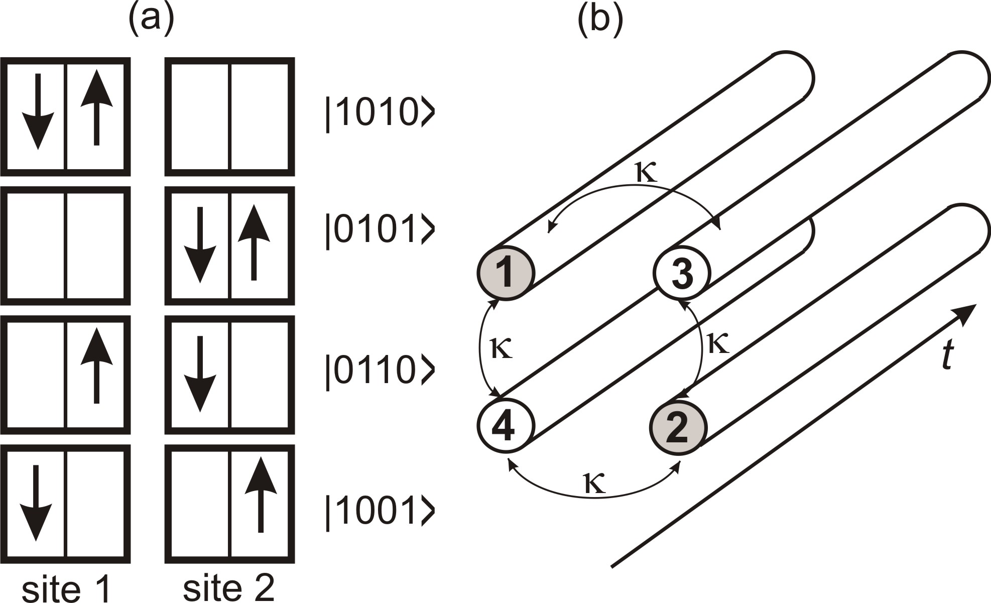
Figure 1: (a) Wannier basis of the two-site Hubbard Hamiltonian corresponding to two electrons with opposite spins, and (b) corresponding optical realization based on four evanescently-coupled optical waveguides. The coupling rate between nearest waveguides is $\kappa$, whereas the propagation constant of the modes of waveguides 1 and 2 is shifted by $U$ from the one of waveguides 3 and 4. The waveguides 1,2,3 and 4 correspond to the four quantum states $|1,0,1,0\rangle$, $|0,1,0,1\rangle$, $|0,1,1,0\rangle$ and $|1,0,0,1\rangle$, respectively.

where $|0\rangle$ is the vacuum state. The state $|\mathbf{n},\mathbf{m}\rangle$ corresponds to $n_{j}$ electrons occupying the site $j$ with spin $\downarrow$ and $m_{j}$ electrons occupying the site $j$ with spin $\uparrow$. Owing to the anti-commutation rules of the Fermi operators, the integers $n_{j}$ and $m_{j}$ can take only the two values $0$ and $1$, according to the Pauli exclusion principle. Hence, the number of all linearly independent Wannier states is $2^{2N}$. If the state vector $|\psi(t)\rangle$ of the system is decomposed on the Wannier basis, $|\psi(t)\rangle=\sum_{\mathbf{n},\mathbf{m}}f(\mathbf{n},\mathbf{m},t)|\mathbf{n},\mathbf{m}\rangle$, the evolution equations for the $2^{2N}$ occupation amplitudes $f(\mathbf{n},\mathbf{m},t)$ are formally given by (assuming $\hbar=1$)

$$i\frac{df(\mathbf{n},\mathbf{m},t)}{dt}=\sum_{\mathbf{s},\mathbf{q}}\langle\mathbf{n},\mathbf{m}|\hat{H}|\mathbf{s},\mathbf{q}\rangle f(\mathbf{s},\mathbf{q},t).$$ (3)

Since the total number of electrons $N_{t}$ and total number of electrons with spin $\uparrow$ ($N_{\uparrow}$) and $\downarrow$ ($N_{\downarrow}$) are conserved quantities for the Hubbard Hamiltonian note , the amplitude equations (3) are decoupled into a set of equations acting on different sub-spaces of the Hilbert space. Each sub-space is defined by the Wannier states with an assigned number of electron $N_{t}=N_{\downarrow}+N_{\uparrow}$, with $N_{\uparrow}$ electrons with spin $\uparrow$ and $N_{\downarrow}$ electrons with spin $\downarrow$; the number of amplitudes in such a subspace is hence $\left(\begin{array}[]{c}N\\ N_{\uparrow}\end{array}\right)\left(\begin{array}[]{c}N\\ N_{\downarrow}\end{array}\right)$. The two-site HM [i.e. $N=2$ in Eq.(1)] provides the simplest and exactly solvable model which can still capture some of the main relevant properties of larger clusters and of the infinite chain. The two-site HM has been investigated by several authors Avella03 ; M1 ; M2 ; M3 ; Kozlov96 ; Fox85 ; Ziegler10 and proposed as a toy model for understanding the binding of molecules like $H_{2}$ M1 ; M2 ; M3 , to model electron-molecular vibration coupling in organic charge-transfer salts Kozlov96 , and to describe the electronic structure in $\pi$ systems Fox85 . Here we propose an optical realization of the two-site Hubbard Hamiltonian based on light transport in evanescently-coupled optical waveguides which is capable of mimicking the temporal dynamics of the Hubbard system in the Wannier basis representation (3). For the two-site Hubbard Hamiltonian, there are 16 possible configurations of electrons on two sites: one with no electrons, four with one electron (an up or down electron on each of the two sites), six with two electrons (one with two up electrons on different sites, one with two down electrons, and four with an up electron and a down electron), four with three electrons, and one with four electrons. The most interesting dynamics is provided by the sub-space consisting of two electrons with opposite spins, i.e. to $N_{t}=2$ and $N_{\uparrow}=N_{\downarrow}=1$, which is spanned by the four states $|1,0,1,0\rangle$, $|0,1,0,1\rangle$, $|0,1,1,0\rangle$ and $|1,0,0,1\rangle$ with amplitudes $c_{1}(t)\equiv f(1,0,1,0,t)$, $c_{2}(t)\equiv f(0,1,0,1,t)$, $c_{3}(t)\equiv f(0,1,1,0,t)$ and $c_{4}(t)\equiv f(1,0,0,1,t)$ [see Fig.1(a)]. In this case, the coupled equations (3) for the amplitudes $c_{l}(t)$ ($l=1,2,3,4$) read explicitly

$$i\frac{d}{dt}\left(\begin{array}[]{c}c_{1}\\ c_{2}\\ c_{3}\\ c_{4}\end{array}\right)=\left(\begin{array}[]{c c c c}U&0&-\kappa&-\kappa\\ 0&U&-\kappa&-\kappa\\ -\kappa&-\kappa&0&0\\ -\kappa&-\kappa&0&0\end{array}\right)\left(\begin{array}[]{c}c_{1}\\ c_{2}\\ c_{3}\\ c_{4}\end{array}\right).$$ (4)

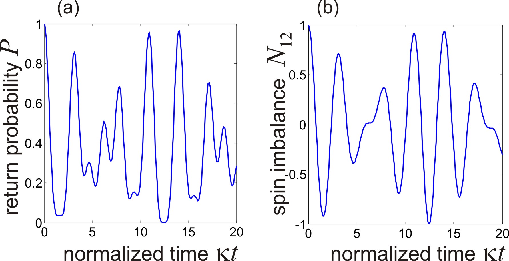
Figure 2: Temporal evolution of (a) the return probability $P(t)$, and (b) the spin imbalance $N_{12}(t)$ for the two-site Hubbard model for $U/\kappa=0.5$. The system is initially prepared in the state $|0,1,1,0\rangle$.

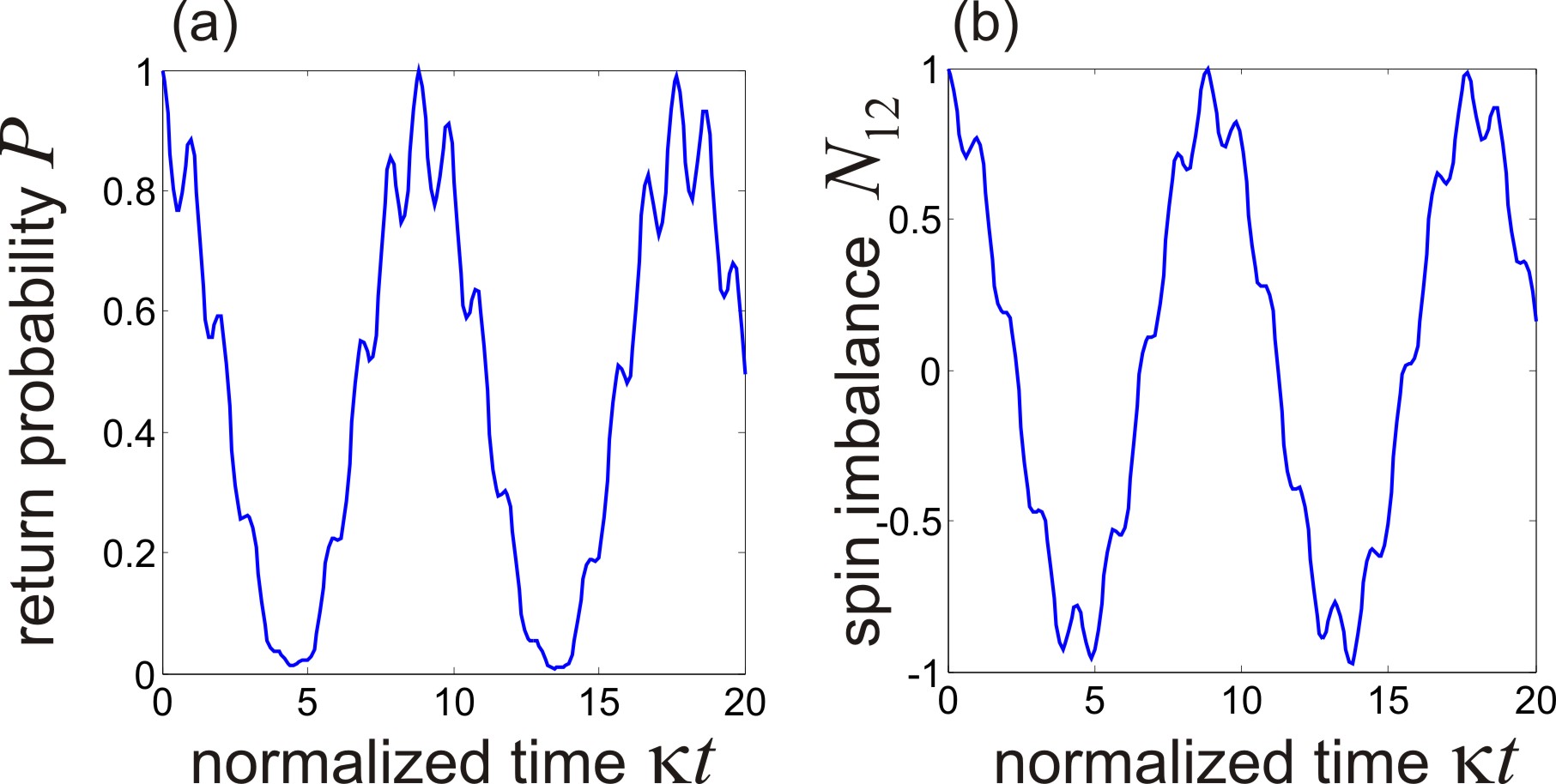
Figure 3: Same as Fig.2, but for $U/\kappa=5$.

An optical realization of the Hamiltonian system (4) is provided by propagation of monochromatic light waves at wavelength $\lambda$ in four evanescently-coupled optical waveguides in the geometrical setting shown in Fig.1(b). In the optical structure, the time $t$ represents the spatial propagation distance along the waveguide axis, whereas the Wannier amplitude $c_{l}$ corresponds to the modal amplitude of light trapped in the $l$-th waveguide ($l=1,2,3,4$). In fact, in the tight-binding approximation the spatial part of the electric field $\mathcal{E}(x,y,t)$ of the optical wave propagating along the $t$ spatial direction of the guiding structure can be written as $\mathcal{E}(x,y,t)\simeq\sum_{l=1}^{4}c_{l}(t)u_{l}(x,y)\exp(2\pi in_{0}t/\lambda)$, where $(x,y)$ are the spatial coordinates transverse to the optical $t$ axis, $u_{l}(x,y)$ is the spatial modal profile of the $l$-th waveguide, and $n_{0}$ is an effective reference mode index. The spatial evolution of the modal amplitudes $c_{l}$ arising from the weak evanescent coupling of adjacent waveguides is governed by coupled mode equations Longhi09LPR ; B01 ; Led1 which are formally analogous to Eqs.(4), provided that the cross-coupling between waveguides 1 and 2, and between waveguides 3 and 4 in Fig.1(b), is negligible. In the optical setting, the hopping rate $\kappa$ entering in Eq.(4) is analogous to the spatial tunneling rate of light waves between two adjacent waveguides arising from evanescent field coupling, whereas the on-site Coulomb interaction strength $U$ corresponds to a shift of the propagation constants of waveguides $1$ and $2$ as compared to waveguides $3$ and $4$ [see Fig.1(b)]. The optical structure shown of Fig.1(b) could be easily realized in fused silica by the recently-developed femtosecond writing technique, in which the propagation constant shift $U$ is realized by varying the writing speed of waveguides (see, for instance, Szameit10 ).

The energies of the two-site Hubbard Hamiltonian can be calculated analytically as the eigenvalues of the $4\times 4$ matrix entering in Eq.(4), and read explicitly (see, for instance, Kozlov96 ) $E_{1}=0$, $E_{2}=U$, $E_{3}=(U/2)+\sqrt{(U/2)^{2}+4\kappa^{2}}$, and $E_{4}=(U/2)-\sqrt{(U/2)^{2}+4\kappa^{2}}$. In the optical analogy, such energies correspond to the propagation constant mismatch of the various supermodes of the coupled waveguides. It is worth noticing that the energy spectrum of the simple two-site HM contains some important physical features of more complex chains, such as the onset of metal-insulator transition in a half-filled linear chain as the parameter $\kappa/U$ is varied Avella03 . To see this, let us consider the limit of small $\kappa/U$, and let us expand the sector of Hilbert space to include all sectors with two electrons by adding the states $|0011\rangle$ and $|1100\rangle$. These states are eigenstates of $\hat{H}$ with eigenvalue 0. All together, the two electron space of the two site HM has four ‘small’ eigenvalues $0$, $0$, $0$ and $(U/2)-\sqrt{(U/2)^{2}+4\kappa^{2}}\simeq-4\kappa^{2}/U$, and two ‘large’ ones $U$ and $(U/2)+\sqrt{(U/2)^{2}+4\kappa^{2}}\simeq U$. The large eigenvalues are associated with eigenvectors whose components have significant mixtures of the states with doubly occupied sites. The existence of the two groups of states whose eigenvalues are separated by $U$ is a reflection of the upper and lower Hubbard bands in a lattice. The ’Mott-Hubbard’ gap in the spectrum gives rise to a metal-insulator transition L2 . For a given initial state $|\psi(t=0)\rangle=|\psi_{0}\rangle$, there are two interesting observables related to the dynamical evolution of the two-site HM, namely the return probability $P(t)=|\langle\psi(t)|\psi_{0}\rangle|^{2}$ and the spin imbalance between the two sites, $N_{12}(t)=(1/2)\langle\psi(t)|\hat{n}_{1,\uparrow}-\hat{n}_{1,\downarrow}+\hat{n}_{2,\downarrow}-\hat{n}_{2,\uparrow}|\psi(t)\rangle$ (see, for instance, Ziegler10 ). The latter describes the exchange dynamics of the two spins $\uparrow$ and $\downarrow$, located at the two sites. As an example, Figs.2 and 3 show a typical behavior of the return probability $P(t)$ and spin imbalance $N_{12}(t)$ for the two-site HM corresponding to a weak ($U/\kappa=0.5$, Fig.2) and a strong ($U/\kappa=5$, Fig.3) on-site Coulomb interaction for a system initially prepared in the Wannier state $|0,1,1,0\rangle$, i.e. for the initial condition $c_{l}(0)=\delta_{l,3}$. In the Wannier basis representation, the return probability $P(t)$ and spin imbalance $N_{12}(t)$ take the simple form

$$P(t)=\sum_{l=1}^{4}|c_{l}^{*}(0)c_{l}(t)|^{2}\;,\;N_{12}(t)=|c_{3}(t)|^{2}-|c_{4}(t)|^{2}.$$ (5)

Note that in the optical analogue the spin imbalance has a very simple meaning: it is just the power imbalance of light between waveguides 3 and 4. Moreover, if the system is initially prepared in one of the Wannier state, the return probability is simply mapped into the fractional optical power trapped in the initially excited waveguide. For example, if the system is initially prepared in the state $|0,1,1,0\rangle$ as in Figs.2 and 3, one has $P(t)=|c_{3}(t)|^{2}$. It is worth noticing that, the optical analogue of the strong on-site Coulomb interaction regime $U/\kappa\gg 1$ (as in Fig.3) corresponds to a nearly-sinusoidal exchange of optical power between waveguides 3 and 4, like in an ordinary synchronous optical direction coupler Yariv . In fact, in the large $U/\kappa$ limit and for the initial condition $c_{1}(0)=c_{2}(0)=0$, the amplitudes $c_{1}$ and $c_{2}$ remain small and can be eliminated from the dynamics by standard perturbation methods. This yields the reduced dynamical equations for the amplitudes $c_{3}$ and $c_{4}$

$$i\frac{dc_{3}}{dt} \simeq-\kappa_{e}c_{4}+\delta c_{3}$$ (6)

$$i\frac{dc_{4}}{dt} \simeq-\kappa_{e}c_{3}+\delta c_{4}$$ (7)

where $\kappa_{e}\equiv 2\kappa^{2}/U$ is an effective coupling constant and $\delta=-\kappa_{e}$ a common propagation constant detuning. Hence light coupling in the four-waveguide structure in the large on-site Coulomb interaction regime is like the one of an ordinary two-waveguide directional coupler, showing Rabi-like exchange of the optical power between the (not directly coupled) waveguides 3 and 4 mediated by the two off-resonance waveguides 1 and 2. The observed oscillatory power exchange between two uncoupled waveguides, arising from indirect coupling via weakly excited off-resonance waveguides, is analogous to the process of two-photon Rabi oscillations observed in Ref.Ornigotti .

In conclusion, a simple classical realization of the two-site Fermi-Hubbard Hamiltonian, based on light propagation in evanescently-coupled optical waveguides, has been theoretically proposed. While previous theoretical and experimental studies on optical simulations of quantum phenomena in solid-state physics have been concerned with single-particle phenomena, here it has been shown that photonics can provide a laboratory tool to visualize and simulate in simple optical settings the dynamical aspects embodied in the physics of interacting fermionic systems. The present study has been focused on a simple Hubbard system, however it is envisaged that photonic simulators of others and more complex models of interacting fermions can be realized. Possible extensions of the present study include the photonic realization of the Hubbard-Holstein Hamiltonian HH , which describes bipolarons dynamics arising from electron-phonon coupling, and the Hubbard-Anderson Hamiltonian Moura describing the dynamics of two electrons on a linear chain with long-range correlated disorder and on-site Hubbard interaction. The Hubbard-Anderson Hamiltonian can be simulated using a two-dimensional square array of waveguides with engineered propagation constants, which can be used to test in an optical setting the interplay between disorder, localization and electron-electron interaction. Phonon-electron coupling dynamics for a two-site Hubbard-Holstein Hamiltonian can be realized by coupling two of the four waveguides of Fig.1(b) with two semi-infinite linear arrays with non-homogeneous hopping rates, which simulate the vibrational (phonon) degrees of freedoms of the two sites.

The authors acknowledge financial support by the Italian MIUR (Grant No. PRIN-2008-YCAAK project ”Analogie ottico-quantistiche in strutture fotoniche a guida d’onda”).

References

- (1) D. Dragoman and M. Dragoman, Quantum-Classical Analogies (Springer, Berlin, 2004).
- (2) S. Longhi, Laser & Photon. Rev. 3, 243 261 (2009).
- (3) D. N. Christodoulides, F. Lederer, and Y. Silberberg, Nature 424, 817 (2003).
- (4) F. Lederer, G.I. Stegeman, D.N. Christodoulides, G. Assanto M. Segev, and Y. Silberberg, Phys. Rep. 463, 1 (2008).
- (5) A. Szameit and S. Nolte, J. Phys. B 43, 163001 (2010).
- (6) U. Peschel, T. Pertsch, and F. Lederer, Opt. Lett. 23, 1701; R. Morandotti, U. Peschel, J. S. Aitchison, H. S. Eisenberg, and Y. Silberberg, Phys. Rev. Lett. 83, 4756 (1999); T. Pertsch, P. Dannberg, W. Elflein, A. Bräuer, and F. Lederer, Phys. Rev. Lett. 83, 4752 (1999); G. Lenz, I. Talanina, and C.M. de Sterke, Phys. Rev. Lett. 83, 963 (1999); N. Chiodo, G. Della Valle, R. Osellame, S. Longhi, G. Cerullo, R. Ramponi, P. Laporta, and U. Morgner, Opt. Lett. 31, 1651 (2006); H. Trompeter, W. Krolikowski, D. N. Neshev, A. S. Desyatnikov, A.A. Sukhorukov, Yu. S. Kivshar, T. Pertsch, U. Peschel, and F. Lederer, Phys. Rev. Lett. 96, 053903 (2006).
- (7) R. Khomeriki and S. Ruffo, Phys. Rev. Lett. 94, 113904 (2005); H. Trompeter, T. Pertsch, F. Lederer, D. Michaelis, U. Streppel, A. Bräuer, and U. Peschel, Phys. Rev. Lett. 96, 023901 (2006); A. Fratalocchi, G. Assanto, K. A. Brzdakiewicz, and M. A. Karpierz, Opt. Lett. 31, 1489 (2006); A. Fratalocchi and G. Assanto, Opt. Express 14, 2021 (2006); S. Longhi, Europhys. Lett. 76, 416 (2006); F. Dreisow, A. Szameit, M. Heinrich, T. Pertsch, S. Nolte, A. Tünnermann, and S. Longhi, Phys. Rev. Lett. 102, 076802 (2009).
- (8) S. Longhi, Opt. Lett. 30, 2137 (2005); S. Longhi, M. Marangoni, M. Lobino, R. Ramponi, P. Laporta, E. Cianci, and V. Foglietti, Phys. Rev. Lett. 96, 243901 (2006); R. Iyer, J. S. Aitchison, J. Wan, M. M. Dignam, and C. M. de Sterke, Opt. Express 15, 3212 (2007); F. Dreisow, M. Heinrich, A. Szameit, S. Döring, S. Nolte, A. Tünnermann, S. Fahr, and F. Lederer, Opt. Express 16, 3474 (2008); A. Szameit, I.L. Garanovich, M. Heinrich, A.A. Sukhorukov, F. Dreisow, T. Pertsch, S. Nolte, A. Tünnermann, and Y.S. Kivshar, Nature Phys. 5, 271 (2009); A. Joushaghani, R. Iyer, J.K.S. Poon, J.S. Aitchison, C.M. de Sterke, J. Wan, and M.M. Dignam, Phys. Rev. Lett. 103, 143903 (2009); S. Longhi, Phys. Rev. B 80, 235102 (2009); G. Della Valle and S. Longhi, Opt. Lett. 35, 673 (2010); A. Szameit, I.L. Garanovich, M. Heinrich, A.A. Sukhorukov, F. Dreisow, T. Pertsch, S. Nolte, A. Tunnermann, S. Longhi, and Y.S. Kivshar, Phys. Rev. Lett. 104, 223903 (2010).
- (9) T. Schwartz, G. Bartal, S. Fishman, and M. Segev, Nature 446, 55 (2007); Y. Lahini, A. Avidan, F. Pozzi, M. Sorel, R. Morandotti, D. N. Christodoulides, and Y. Silberberg, Phys. Rev. Lett. 100, 013906 (2008).
- (10) K. Shandarova, C.E. Ruter, D. Kip, K.G. Makris, D.N. Christodoulides, O. Peleg, and M. Segev, Phys. Rev. Lett. 102, 123905 (2009).
- (11) A. Szameit, F. Dreisow, M. Heinrich, R. Keil, S. Nolte, A. Tunnermann, and S. Longhi, Phys. Rev. Lett. 104, 150403 (2010).
- (12) J. Hubbard, Proc. Roy. Soc. A 276, 238 (1963).
- (13) The Hubbard Model, edited by M. Rasetti (World Scientific, Singapore, 1991); The Hubbard Model: A Reprint Volume, edited by A. Montorsi (World Scientific, Singapore, 1992).
- (14) F.H.L. Essler, H. Frahm, F. Göhmann, A. Klümper, and V.E. Korepin, The One-Dimensional Hubbard Model (Cambridge University Press, Cambridge, 2005).
- (15) A.B. Harris and R.V. Lange, Phys. Rev. 157, 295 (1967); H. Shiba and P.A. Pincus, Phys. Rev. B 5, 1966 (1972); D. Cabib and T.A. Kaplan, Phys. Rev. B 7, 2199 (1973).
- (16) A. Avella, F. Mancini, and T. Saikawa, Eur. Phys. J. B 36, 445 (2003).
- (17) P. Fulde, J. Keller, and G. Zwicknagel, Solid State Phys. 41, 1, (1988); L.C. Andreani, S. Fraizzoli, and H. Beck, Solid State Commun. 77, 635 (1991).
- (18) P. Ziesche, O. Gunnarsson, W. John,and Hans Beck, Phys. Rev. B 55, 10270 (1997).
- (19) R. J. Magyar, Phys. Rev. B 79, 195127 (2009).
- (20) M.E. Kozlov, V.A. Ivanov, and K. Yakushi, Phys. Lett. A 214, 167 (1996).
- (21) M.A. Fox and F.A. Matsen, J. Chem. Educ. 62, 369 (1985).
- (22) K. Ziegler, Phys. Rev. A 81, 034701 (2010).
- (23) S. Longhi, J. Phys. B 44, 051001 (2011); S. Longhi, Phys. Rev. A 83, 034102 (2011).
- (24) This is because the electrons are conserved in number and cannot change their spin when they hop.
- (25) A. Yariv, Optical Electronics, 4th ed. (Saunders College Publishing, New York, 1991), pp. 519-529.
- (26) M. Ornigotti, G. Della Valle, T. Toney Fernandez, A Coppa, V. Foglietti, P. Laporta, and S Longhi, J. Phys. B 41 , 085402 (2008).
- (27) M. Berciu, Phys. Rev. B 75, 081101(R) (2007).
- (28) W.S. Dias, E.M. Nascimento, M.L. Lyra, and F.A.B.F. de Moura, Phys. Rev. B 81, 045116 (2010).