Classical simulation of the Hubbard-Holstein dynamics with optical waveguide lattices

Abstract

A classical analog simulator of the two-site Hubbard-Holstein model, describing the dynamics of two correlated electrons coupled with local phonons, is proposed based on light transport in engineered optical waveguide arrays. Our photonic analog simulator enables to map the temporal dynamics of the quantum system in Fock space into spatial propagation of classical light waves in the evanescently-coupled waveguides of the array. In particular, in the strong correlation regime the periodic temporal dynamics, related to the excitation of Holstein polarons with equal energy spacing, can be visualized as a periodic self-imaging phenomenon of the light beam along the waveguide array and explained in terms of generalized Bloch oscillations of a single particle in a semi-infinite inhomogeneous tight-binding lattice.

I Introduction

In recent years, there has been a renewed and increasing interest in the development of quantum analog simulators, i.e. controllable quantum systems that can be used to imitate other quantum systems (see, for instance, Nori and references therein). Quantum analog simulators would be very useful for a wide variety of problems in physics, chemistry, and biology. In particular, they have proven to be able to tackle complex quantum many-body problems in condensed-matter physics Lewenstein ; Bloch ; i0 , such as correlated electrons or quantum magnetism. Quantum analog simulators are also useful to test predictions or states of matter difficult to access experimentally in the originally proposed system, such as dynamical and extreme conditions Nori . Recent realizations of quantum analog simulators of many-body problems have been based mainly on atoms Lewenstein ; a1 ; a2 ; a3 , trapped ions i0 ; i1 ; i2 ; i3 , nuclear magnetic resonance mr1 , and single photons ppp1 ; ppp2 . As compared to quantum simulators based on atoms or ions, those employing single photons offer the feasibility to individually address and access the dynamics of single particles, and are thus suited to simulate the physics of few interacting particles ppp2 . Unlike electrons, photons do not interact with each other, especially at the few photon level, and hence for the simulation of quantum many-body problems of condensed-matter physics particle interaction has to be introduced in a suitable manner. At the few photon level, interaction is generally mimicked using purely linear optical systems by measurement-induced nonlinearity Milburn . In this way, simplified toy models of many-body condensed matter physics have been simulated, such as frustrated Heisenberg dynamics in a spin-1/2 tetramer ppp2 . On the other hand, propagation of classical light in waveguide-based optical lattices has provided an experimentally accessible test bed to mimic in a purely classical setting single-particle coherent phenomena of solid-state physics LonghiLPR ; Szameit10 , such as Bloch oscillations BO , dynamic localization DL , and Anderson localization AL to mention a few. Recently, the possibility to simulate Bose-Hubbard and Fermi-Hubbard models of few interacting bosons or fermions in coupled-waveguide linear optical structures using classical light beams has been proposed as well Longhi1 ; Longhi2 . The main idea is that the temporal evolution of a few interacting particles in Fock space can be conveniently mapped into linear spatial propagation of discretized light Lederer in engineered evanescently-coupled optical waveguides. As compared to quantum simulators using single photons, atoms or trapped ions, such a kind of classical simulators of quantum many-body problems using classical light would benefit for the much simpler experimental implementation, the rather unique possibility to provide a direct access and visualization of the temporal dynamics of the quantum system in Fock space, and the ability to prepare the system in a rather arbitrary (for example highly entangled) state.
In condensed-matter, strong correlation effects and localization can occur in metallic systems due both to strong electron-electron(e-e) interactions and strong electron-phonon (e-ph) coupling. Evidences of strong e-ph interactions have been reported in such important materials as cuprates, fullerides, and manganites (see, e.g., cuprates and references therein). The interplay of e-e and e-ph interactions in these correlated systems leads to coexistence of or competition between various phases such as superconductivity, charge-density-wave or spin-density-wave phases, or formation of novel non-Fermi liquid phases, polarons, bipolarons, etc. One of the simplest theoretical model that accounts for the interplay between these two types of interactions is the Holstein-Hubbard (HH) model HH0 ; HH1 ; HH2 . Even though the HH model provides an oversimplified description of both e-e and e-ph interactions, it retains what are thought to be the relevant ingredients of a system in which electrons experience simultaneously an instantaneous short-range repulsion and a phonon-mediated retarded attraction. Actually, in spite of its formal simplicity, it is not exactly solvable even in one dimension. As quantum simulators of Fermi-Hubbard models, based on either fermionic atoms in optical lattices Bloch ; FHP or electrons in artificial quantum-dot crystals CQD , have attracted great interest, analog simulators of HH models have not received special attention yet. The smallest configuration for studying and simulating the HH dynamics is the dimer HH model, which describes two correlated electrons hopping between two adjacent sites HH2 . In In this work, a classical analog simulator is theoretically proposed for the two-site HH model, based on light transport in engineered waveguide lattices, which is capable of reproducing the temporal dynamics of the quantum model in Fock space as spatial beam evolution in the photonic lattice. The paper is organized as follows. In Sec.II, the HH model is briefly reviewed, and the dynamical equations of Fock-state amplitudes are derived. In Sec.III, a classical analog simulator based on light transport in engineered waveguide arrays is described, and numerical results are presented for waveguide structures that simulate the HH model for different electron correlation regimes. In particular, in the strong correlation regime the quasi-periodic temporal dynamics, related to the excitation of Holstein polarons, is visualized as a periodic self-imaging phenomenon of the light beam that propagates along the waveguide array and explained in terms of generalized Bloch oscillations of a single particle in an inhomogeneous biased tight-binding lattice. Finally, in Sec. IV the main conclusions are outlined.

II The Hubbard-Holstein model: Fock-space representation

II.1 The two-site Hubbard-Holstein model

The two-site HH model describes two correlated electrons hopping between two adjacent sites (a diatomic molecule), each of which exhibits an optical mode with frequency $\Omega$. This model has been often used in condensed-matter physics as a simplified toy model to describe some basic features of polaron and bipolaron dynamics (see, for instance, HH2 ). The two-site HH Hamiltonian can be separated into two terms HH2 . One describes a shifted oscillator that does not couple to the electronic degrees of freedom, and can be thus disregarded. The other describes the effective e-ph system where phonons couple directly with the electronic degrees of freedom. The corresponding Hamiltonian, with $\hbar=1$, reads explicitly HH2

$$\hat{H}=\hat{H}_{e}+\hat{H}_{ph}+\hat{V}_{e-ph}$$ (1)

where

$$\hat{H}_{e} = -t\sum_{\sigma=\uparrow,\downarrow}\left(\hat{c}^{{\dagger}}_{1,\sigma}\hat{c}_{2,\sigma}+\hat{c}^{{\dagger}}_{2,\sigma}\hat{c}_{1,\sigma}\right)+$$ (2)

$$+ U\left(\hat{n}_{1,\uparrow}\hat{n}_{1,\downarrow}+\hat{n}_{2,\uparrow}\hat{n}_{2,\downarrow}\right)$$

$$\hat{H}_{ph} = \Omega\hat{b}^{{\dagger}}\hat{b}$$ (3)

$$\hat{V}_{e-ph} = \frac{g}{\sqrt{2}}\left(\hat{n}_{1}-\hat{n}_{2}\right)\left(\hat{b}+\hat{b}^{{\dagger}}\right).$$ (4)

In the previous equations, $\hat{c}^{{\dagger}}_{i,\sigma}$ ($\hat{c}_{i,\sigma}$) are the fermionic creation (annihilation) operators for the electron at site $i$ with spin $\sigma$ ($i=1,2$, $\sigma=\uparrow,\downarrow$), $\hat{n}_{i,\sigma}=\hat{c}^{{\dagger}}_{i,\sigma}\hat{c}_{i,\sigma}$ and $\hat{n}_{i}=\hat{n}_{i,\uparrow}+\hat{n}_{i,\downarrow}$ are the electron occupation numbers, $g$ is the on-site e-ph coupling strength, $t$ is the hopping amplitude between adjacent sites, $U$ is the on-site Coulomb interaction energy, and $\hat{b}^{{\dagger}}$ ($\hat{b}$) is creation (annihilation) bosonic operator for the oscillator. For the two-site two-electron system there are six electronic states. Three of these states are degenerate, with zero energy $\hat{H}_{e}|\psi_{Ti}\rangle=0$ ($i=1,2,3$), and belong to the triplet states as follows:

$$|\psi_{T1}\rangle = \hat{c}^{{\dagger}}_{1,\uparrow}\hat{c}^{{\dagger}}_{2,\uparrow}|0\rangle_{e}$$ (5)

$$|\psi_{T1}\rangle = \frac{1}{\sqrt{2}}\left(\hat{c}^{{\dagger}}_{1,\uparrow}\hat{c}^{{\dagger}}_{2,\downarrow}+\hat{c}^{{\dagger}}_{1,\downarrow}\hat{c}^{{\dagger}}_{2,\uparrow}\right)|0\rangle_{e}$$ (6)

$$|\psi_{T3}\rangle = \hat{c}^{{\dagger}}_{1,\downarrow}\hat{c}^{{\dagger}}_{2,\downarrow}|0\rangle_{e}.$$ (7)

The triplet states are not coupled with the $b$-oscillator, and can be thus disregarded. The three other eigenstates of $\hat{H}_{e}$, denoted by $|-\rangle$, $|s+\rangle$ and $|s-\rangle$, are constructed from the singlet states and read explicitly

$$|-\rangle = \frac{1}{\sqrt{2}}\left(\hat{c}^{{\dagger}}_{1,\uparrow}\hat{c}^{{\dagger}}_{1,\downarrow}-\hat{c}^{{\dagger}}_{2,\uparrow}\hat{c}^{{\dagger}}_{2,\downarrow}\right)|0\rangle_{e}$$ (8)

$$|s+\rangle = \sin\theta|s\rangle-\cos\theta|+\rangle$$ (9)

$$|s-\rangle = \cos\theta|s\rangle+\sin\theta|+\rangle$$ (10)

where we have set

$$|+\rangle = \frac{1}{\sqrt{2}}\left(\hat{c}^{{\dagger}}_{1,\uparrow}\hat{c}^{{\dagger}}_{1,\downarrow}+\hat{c}^{{\dagger}}_{2,\uparrow}\hat{c}^{{\dagger}}_{2,\downarrow}\right)|0\rangle_{e}$$ (12)

$$|s\rangle = \frac{1}{\sqrt{2}}\left(\hat{c}^{{\dagger}}_{1,\uparrow}\hat{c}^{{\dagger}}_{2,\downarrow}-\hat{c}^{{\dagger}}_{1,\downarrow}\hat{c}^{{\dagger}}_{2,\uparrow}\right)|0\rangle_{e}$$ (13)

and

$$\cos\theta=\sqrt{\frac{1}{2}\left(1+\frac{U}{\sqrt{U^{2}+16t^{2}}}\right)}.$$ (14)

For these states one has $\hat{H}_{e}|-\rangle=U|-\rangle$ and $\hat{H}_{e}|s\pm\rangle=E_{\pm}|s\pm\rangle$, where

$$E_{\pm}=\frac{U\pm\sqrt{U^{2}+16t^{2}}}{2}.$$ (15)

The e-ph interaction term $\hat{V}_{e-ph}$ couples the electronic eigenstates $|-\rangle$ and $|s\pm\rangle$ of $\hat{H}_{e}$ with the phonon states $|n\rangle_{ph}=(1/\sqrt{n!})\hat{b}^{{\dagger}n}|0\rangle_{ph}$ of $\hat{H}_{ph}$.

II.2 Fock-space representation

In order to realize a photonic analog simulator of the HH Hamiltonian, it is worth expanding the state vector $|\psi(t)\rangle$ of the electron-phonon system in Fock space as follows

$$|\psi_{t}\rangle=\sum_{n=0}^{\infty}\left[f_{n}(t)|-\rangle+g_{n}|s+\rangle-h_{n}(t)|s-\rangle\right]\bigotimes|n\rangle_{ph}.$$ (16)

The evolution equations for the amplitude probabilities $f_{n}$, $g_{n}$ and $h_{n}$ in Fock space, as obtained from the Schrödinger equation $i\partial_{t}|\psi(t)\rangle=\hat{H}|\psi(t)\rangle$, read explicitly

$$i\frac{df_{n}}{dt} = (U+\Omega n)f_{n}-\kappa_{n}g_{n-1}-\kappa_{n+1}g_{n+1}-\rho_{n}h_{n-1}+$$ (17)

$$- \rho_{n+1}h_{n+1}$$

$$i\frac{dg_{n}}{dt} = (E_{+}+n\Omega)g_{n}-\kappa_{n}f_{n-1}-\kappa_{n+1}f_{n+1}$$ (18)

$$i\frac{dh_{n}}{dt} = (E_{-}+n\Omega)h_{n}-\rho_{n}f_{n-1}-\rho_{n+1}f_{n+1}\$$ (19)

($n=0,1,2,3,...$), where we have set

$$\kappa_{n}=\sqrt{2n}g\cos\theta\;,\;\rho_{n}=\sqrt{2n}g\sin\theta$$ (20)

and where we have assumed $f_{-1}=g_{-1}=h_{-1}=0$ for definiteness.

III Photonic analog simulator

III.1 Waveguide array design

Equations (17-19) govern the temporal dynamics in Fock space of the HH Hamiltonian, and their optical implementation can be achieved using a simple linear optical network because the coupled equations of the Fock-state amplitudes are linear equations. Let us first notice that Eqs.(17-19) decouple into two sets of equations involving the former the amplitudes $\{f_{2n}(t),g_{2n+1}(t),h_{2n+1}(t)\}$, the latter the amplitudes $\{f_{2n+1}(t),g_{2n}(t),h_{2n}(t)\}$ ($n=0,1,2,3,...)$. A schematic of the optical networks that provide analog simulators of the two sets of equations are depicted in Fig.1. Their physical implementation can be obtained by using either arrays of coupled optical waveguides with engineered coupling rates and propagation constants, where the temporal evolution of the Fock-state amplitudes is mapped into spatial propagation of the light fields along the axis of the various waveguides, or arrays of coupled optical cavities with engineered coupling rates and resonance frequencies, in which the temporal evolution of the Fock-state amplitudes is mimicked by the temporal evolution of the light field stored in the various cavities. Owing to the current technological advances in manufacturing engineered arrayed waveguides and related imaging techniques based on femtosecond laser writing (see, for instance, Szameit10 and references therein), we will consider here specifically an optical analog simulator of the HH model based on propagation of monochromatic light waves in coupled optical waveguides. Moreover, since the dynamics of the two networks of Fig.1 is decoupled, without loss of generality we can limit to consider initial conditions that excite only one of them, for example the one corresponding to Fig.1(a).

Light transport of a classical monochromatic field at wavelength $\lambda$ in a weakly-guiding arrays of coupled optical waveguides with a straight optical axis $z$, in the geometrical setting schematically depicted in Fig.1(a), is described by the optical Schödinger equation for the electric field envelope $\phi(x,y,z)$ LonghiLPR

$$i\lambdabar\frac{\partial\phi}{\partial z}=-\frac{\lambdabar^{2}}{2n_{s}}\left(\frac{\partial^{2}\phi}{\partial x^{2}}+\frac{\partial^{2}\phi}{\partial y^{2}}\right)+V(x,y)\phi,$$ (21)

where $\lambdabar=\lambda/(2\pi)$ is the reduced wavelength of photons, $n_{s}$ is the refractive index of the substrate at wavelength $\lambda$, $V(x,y)\simeq n_{s}-n(x,y)$ is the so-called optical potential, and $n(x,y)$ is the refractive index profile of the optical structure defining the various waveguide channels. Let $h(x,y)$ be the normalized profile of the waveguide core, which is typically assumed to be circularly-shaped with a super-Gaussian profile of radius $a$, $(x_{i},y_{i})$ the position of the $i$-th waveguide of the array, and $\Delta n_{i}$ its index change from the cladding (substrate) region. One can thus write:

$$V(x,y)\simeq-\sum_{i}\Delta n_{i}h(x-x_{i},y-y_{i}).$$ (22)

In the tight-binding approximation, the electric field envelope can be expanded as a superposition of the fundamental guided modes of each waveguide with amplitudes that vary slowly along $z$ due to evanescent mode-coupling and propagation constant mismatch Yariv . In the nearest-neighboring approximation, the resulting coupled-mode equations, obtained by using e.g. a variational procedure LonghiPLA , are precisely of the form (17-19), provided that cross-couplings among waveguides are negligible and the temporal variable $t$ in the quantum HH model is replaced by the spatial propagation distance $z$. If needed, to avoid cross-couplings suitable high-index waveguides (or off-resonance resonators) could be inserted into the structure, as shown in Fig.1(a). The coupling constants $\kappa_{n}$, $\rho_{n}$ entering in the equations (17-19) are basically determined by the waveguide separation via an overlapping integral of the evanescent fields LonghiPLA , whereas the propagation constant shifts $U+n\Omega$ and $E_{\pm}+n\Omega$ can be controlled by the core index changes $\Delta n_{n}$ of the various waveguides. Let us consider, as an example, propagation of light waves at wavelength $\lambda=633$ nm (red) in waveguides written by femtosecond laser pulses in fused silica Szameit10 , for which $n_{s}\simeq 1.45$. The normalized core profile of the waveguides is assumed to be super-Gaussian-shaped with a core radius $a=2.5\;\mu$m, namely $h(x,y)=\exp[-(x^{2}+y^{2})^{2}/a^{4}]$; the index change of the various waveguides is taken to be $\Delta n_{i}=\Delta n+\delta n_{i}$, where $\Delta n=2\times 10^{-3}$ is a reference index change and $\delta n_{i}$ a small perturbation, as compared to $\Delta n$, needed to realize the propagation constant shifts. For such waveguides, the coupling constant $\kappa(d)$ (in units of ${\rm mm}^{-1}$) between two waveguides placed at a distance $d$ (in units of $\mu$m) turns out to be very well approximated, for distances $d>\sim 6\mu$m, by the exponential relation LonghiPRB2009 $\kappa=A\exp(-\gamma d)$, with $A\simeq 24.6\;{\rm mm}^{-1}$ and $\gamma\simeq 0.466\;\mu{\rm m}^{-1}$. Similarly, the propagation constant shift $\sigma(\delta n)$ of the fundamental waveguide mode induced by an index change $\delta n$, added to $\Delta n$, is very well approximated (for $|\delta n|\ll\Delta n$) by the relation $\sigma(\delta n)\simeq-1.7\delta n/\lambdabar$. Using such relations, one can thus design a waveguide array, with controlled waveguide separation and index changes, that realizes the desired coupling rates $\kappa_{n}$, $\rho_{n}$ [given by Eq.(20)] and propagation constant shifts $U+n\Omega$ and $E_{\pm}+n\Omega$. The total number of waveguides needed to simulate the HH model is basically determined by the largest phonon number $n$ that will be excited in the dynamics.

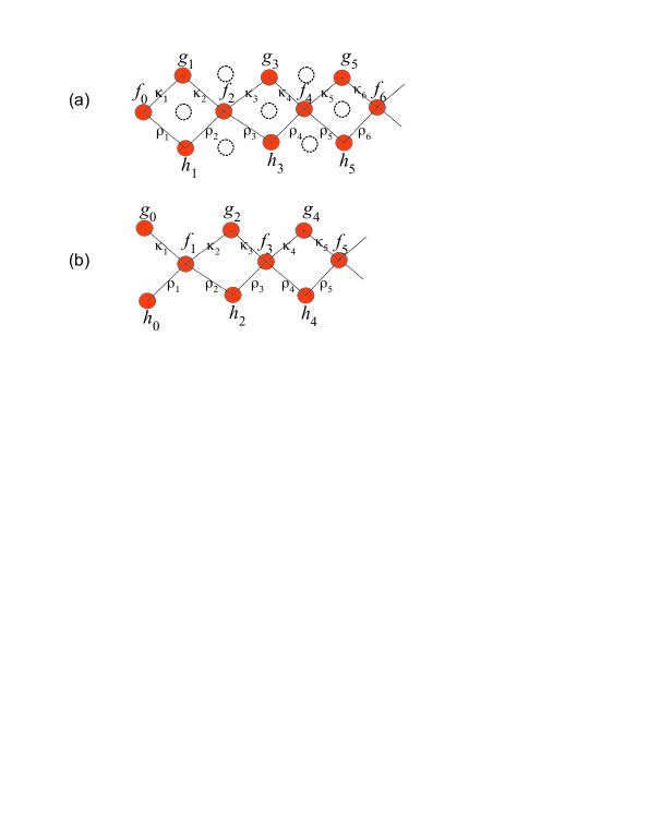
Figure 1: Schematic of the optical networks that realize analog simulators of the two sets of equations (17-19) for $n$ even [Fig.1(a)] and $n$ odd [Fig.1(b)]. The filled circles indicate either optical waveguides or optical cavities (resonators) that are coupled by weak evanescent field. The optical elements depicted in Fig.1(a) by dotted circles indicate high-index core waveguides (or off-resonance cavities) that might be inserted, if needed, to avoid cross coupling among the optical elements in the network.

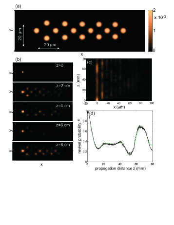
Figure 2: Optical simulations of the HH model in Fock space for parameter values $g=0.1\;\rm{mm}^{-1}$, $t=0.1\;\rm{mm}^{-1}$, $\Omega=0.1\;\rm{mm}^{-1}$, and $U=0$ (uncorrelated electrons). (a) Refractive index profile $n(x,y)-n_{s}$ of the double-chain zig-zag waveguide array. (b-d) Dynamical evolution of the system corresponding to the initial state $|\psi(0)\rangle=|-\rangle\bigotimes|0\rangle_{ph}$. In (b) a snapshot of the intensity light pattern $|\phi(x,y,z)|^{2}$ is shown for a few propagation distances $z$, whereas in (c) a snapshot of $\int dy|\phi(x,y,z)|^{2}$ in the $(x,z)$ plane is depicted. Figure (d) shows the behavior of the return probability $P(z)=|\langle\psi(0)|\psi(z)\rangle|^{2}=|f_{0}(z)|^{2}$ numerically obtained from the solution of the optical Schrödinger equation (solid curve) and from the HH model (thin solid curve).

III.2 Numerical results

In this section we provide a few examples of photonic simulations of the temporal dynamics of the HH Hamiltonian in Fock space, based on light transport in waveguide arrays engineered following the procedure outlined in the previous subsection, and compare the numerical results obtained by the full numerical analysis the optical Schrödinger equation (21) with those predicted by the coupled-mode equations (17-19). As an initial condition, we will assume the system to be in the state $|\psi(0)\rangle=|-\rangle\bigotimes|0\rangle_{ph}$, corresponding to excitation of zero phonon modes and to the two electrons being in the entangled state $|-\rangle=(1/\sqrt{2})(\hat{c}^{{\dagger}}_{1,\uparrow}\hat{c}^{{\dagger}}_{1,\downarrow}-\hat{c}^{{\dagger}}_{2,\uparrow}\hat{c}^{{\dagger}}_{2,\downarrow})|0\rangle$, i.e. the two electrons occupying the same (either left or right) potential well with opposite spins. For such an initial state, according to Eq.(16) the initial conditions for the Fock-state amplitudes are given by $f_{n}(0)=\delta_{n,0}$ and $g_{n}(0)=h_{n}(0)=0$. Such an initial condition simply corresponds to the excitation of the left boundary waveguide in the semi-array of Fig.1(a). The fractional light powers trapped in the various waveguides of the array at different propagation distances $z$ provide a direct mapping of the temporal evolution of the occupation probabilities $|f_{n}|^{2}$, $|g_{n}|^{2}$ and $|h_{n}|^{2}$ of the quantum HH Hamiltonian in Fock space. To monitor the temporal dynamics of the HH model, we mainly use as a dynamical variable the return probability $P(t)=|\langle\psi(0)|\psi(t)\rangle|^{2}=|f_{0}(t)|^{2}$. In our optical simulator, such a variable simply corresponds to the fractional light power that remains in the initially excited boundary waveguide. In the simulations, we assumed constant values of ${\it e-ph}$ coupling $g=0.1\;\rm{mm}^{-1}$ and hopping rate $t=0.1\;\rm{mm}^{-1}$, whereas a few values of the on-site ${\it e-e}$ Coulomb energy $U$ are considered, corresponding to three different correlation regimes: absence of correlation ($U=0$), moderate correlation regime ($U$ comparable with the hopping rate $t$); and strong-correlation regime ($U$ much larger than $t$) note .

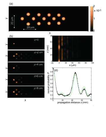
Figure 3: Same as Fig.2, but in the intermediate correlation regime ($U=0.2\;\rm{mm}^{-1}$).

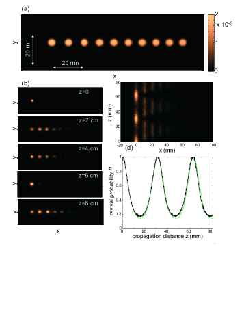
Figure 4: Same as Fig.2, but in the strong correlation regime ($U=10\;\rm{mm}^{-1}$). The oscillation frequency is now $\Omega=0.2\;\rm{mm}^{-1}$.

Figure 2 shows the results obtained for uncorrelated electrons ($U=0$) and for an oscillator frequency $\Omega=0.1\;\rm{mm}^{-1}$. In this case, one has $\cos\theta=\sin\theta=1/\sqrt{2}$, and thus $\kappa_{n}=\rho_{n}$. The refractive index profile $[n(x,y)-n_{s}]$ of the waveguide array is depicted in Fig.2(a). The array comprises $16$ waveguides arranged in two zig-zag chains with non-uniform spacings. The evolution of the light intensity along the array is shown in Figs.2(b) and (c). In particular, in Fig.2(b) a snapshot of the intensity light distribution $|\phi(x,y,z)|^{2}$ is depicted for a few propagation distances (up to $z=8$ cm) as obtained by numerical simulations of the optical Schrödinger equation (21), whereas in Fig.2(c) the snapshot of $\int dy|\phi(x,y,z)|^{2}$ in the $(x,z)$ plane is shown. Note that a relatively small number of waveguides ($\sim 13$) are excited in the dynamics. The corresponding behavior of the return probability $P(z)$ is depicted in Fig.2(d) (solid curve) and compared with the behavior obtained by direct numerical analysis of the HH equations (17-19) (thin solid curve). Note that, even though in our optical network high-index waveguides to avoid weak cross couplings have not been inserted, the agreement with the HH model [Eqs.(17-19)] is rather satisfactory. Figure 3 shows similar results obtained in the moderate correlated regime ($U=0.2\;{\rm mm}^{-1}$), corresponding to $\cos\theta\simeq 0.851$, $\sin\theta\simeq 0.526$. Note that in this case $\kappa_{n}\neq\rho_{n}$, and thus the two zig-zag chains forming the array are noticeably asymmetric.
The strong correlation regime is attained when the on-site interaction strength $U$ is much larger than the hopping amplitude $t$, corresponding to $\cos\theta\simeq 1$ and $\sin\theta\simeq 0$. In this case $\rho_{n}\simeq 0$ and thus the phonon modes are coupled to the electronic degree of freedoms solely via the two dressed states $|-\rangle$ and $|s+\rangle\simeq-|+\rangle$, whose energy levels are nearly degenerate and equal to $U$ and $E_{+}\simeq U(1+4t^{2}/U^{2})$, respectively. In Fock space, the ${\it e-ph}$ coupling dynamics is thus reduced to the coupled equations for the occupation amplitudes $f_{n}$ and $g_{n}$, namely [see Eqs.(17) and (18)]

$$i\frac{df_{n}}{dt} = (U+\Omega n)f_{n}-\kappa_{n}g_{n-1}-\kappa_{n+1}g_{n+1}$$ (23)

$$i\frac{dg_{n}}{dt} = (E_{+}+n\Omega)g_{n}-\kappa_{n}f_{n-1}-\kappa_{n+1}f_{n+1}$$ (24)

where $k_{n}=\sqrt{2n}g$. Correspondingly, the optical analog simulator reduces to a simple linear chain of waveguides with non-uniform spacing, as shown in Fig.4(a). An example of optical simulation of the HH model in the strong correlation regime is shown in Fig.4 for parameter values $g=0.1\;\rm{mm}^{-1}$, $t=0.1\;\rm{mm}^{-1}$, $\Omega=0.2\;\rm{mm}^{-1}$ and $U=10\;\rm{mm}^{-1}$. Note that the dynamics of occupation amplitudes shows in this case a typical periodic behavior with a period given by $2\pi/\Omega$. In our optical simulator, the periodic revival is clearly visualized by the self-imaging property of the waveguide array, in which the initial light periodically returns into the initially-excited waveguide [see Fig.4(c)]. Such a periodic behavior can be explained after observing that, in the strong correlation regime $U\rightarrow\infty$, the phonon modes $|n\rangle_{ph}$ couple solely to two dressed electronic states $|-\rangle$ and $|+\rangle$. Neglecting the small energy shift $(E_{+}-U)$ of dressed levels $|-\rangle$ and $|+\rangle$, the energy levels of the ${\it e-ph}$ coupled system [the eigenvalues of Eqs.(23) and (24) with $E_{+}=U$] is analogous to a Wannier-Stark ladder with energy spacing $\Omega$, namely one has $E_{l}=U+l\Omega-2g^{2}/\Omega$ ($l=0,1,2,3,...$). In fact, in this limit the HH model is equivalent to a two-site tunneling system strongly coupled to a quantum harmonic oscillator, such as the two-site Holstein model in atomic (strong ${\it e-ph}$ coupling) limit H , describing the hopping dynamics of one electron in a two-site potential interacting with local phonon modes, or the Jaynes-Cummings model of quantum optics, describing the interaction of a two-level atom with a quantized oscillator in the so-called deep strong coupling regime JC . In the atomic (strong-coupling) limit, i.e. for a vanishing hopping rate, the Holstein model is exactly integrable using a Lang-Firsov transformation HH0 ; Fir , yielding an equally-spaced discrete energy spectrum corresponding to small Holsten polaron modes . In our optical realization, the equally-spaced energy spectrum is responsible for the periodic self-imaging of the optical beam as it propagates along the array, with a spatial period $\ 2\pi/\Omega$. In our realization of the HH model in Fock space, the periodic self-imaging effect can be explained in terms of generalized Bloch oscillations of a single particle in a non-homogeneous tight-binding lattice with a dc bias. In fact, the tight-binding lattice realization of the HH model in the strong correlation regime, as described by Eqs.(23) and (24) with $E_{+}\simeq U$, belongs to a class of exactly-solvable lattice models which shows an equally-spaced Wannier-Stark ladder spectrum, as shown in Ref.LonghiSELF . In this lattice model, the dc biased in represented by the linear gradient terms $n\Omega$ in Eqs.(23) and (24), and Bloch oscillations are not washed out in spite of lattice truncation and non-homogeneity of hopping rates Ref.LonghiSELF .. If the small energy shift between the dressed energy states $|-\rangle$ and $|+\rangle$ is taken into account, the revival (self-imaging) dynamics would be only approximate because the energy levels of $\hat{H}$ are no more exactly equally spaced (see, for instance, JC ). However, for the parameter values used in the simulation of Fig.4, washing out of the self-imaging would be visible after several self-imaging periods, and it is thus not observed in the figure.

IV Conclusions

In this work, a classical analog simulator of the Hubbard-Holstein model, describing electron-phonon coupling in presence of electron correlations, has been theoretically proposed based on light transport in engineered optical waveguide lattices. Here a toy model has been presented by considering a diatomic molecule, i.e. the two-site two-electron HH model, which describes two correlated electrons hopping between two adjacent sites. Like quantum simulators based on single photons in linear optical networks ppp2 , the kind of classical simulators proposed here is suited to mimic few interacting particles solely, rather than many-particles like quantum simulators based on trapped atoms or ions. Nevertheless, our classical simulator offers the rather unique possibility to visualize the temporal dynamics of the quantum system in Fock space (rather than in real space) and to mimic dynamical evolutions of quite arbitrary and controllable initial states, such as entangled states, which could be not accessible in condensed-matter systems. Simulation of the HH model in Fock space also helps to get new physical insights into certain dynamical aspects of the HH model. For instance, in the strong correlation regime the periodic temporal dynamics exhibited by the HH Hamiltonian, related to the excitation of Holstein polarons, can be explained in terms of generalized Bloch oscillations of a single particle in a semi-infinite inhomogeneous tight-binding lattice, a result which was not noticed in previous studies of HH models. It is envisaged that the present work could stimulate the search for and the experimental demonstration of further classical simulators of many-body problems, involving other types of interactions and even beyond the two-site toy model. For example, light transport in two-dimensional photonic lattices can simulate in Fock space the hopping dynamics of two correlated electrons on a one-dimensional lattice, and can be exploited to visualize such phenomena as correlated tunneling of bound electron-electron molecules and their coherent motion under the action of dc or ac fields, such as Bloch oscillations and dynamic localization of strongly correlated particles ex1 .

- (1) I. Buluta and F. Nori, Science 326, 108 (2009).
- (2) M. Lewenstein, Adv. Phys. 56, 243 (2007).
- (3) I. Bloch, J. Dalibard, and W. Zwerger, Rev. Mod. Phys. 80, 885 (2008).
- (4) M. Johanning, A. F Varon and C. Wunderlich, J. Phys. B 42, 154009 (2009).
- (5) M. Greiner, O. Mandel, T. Esslinger, T.W. Hansch, and I. Bloch, Nature 415, 39 (2002).
- (6) S. Trotzky, L. Pollet, F. Gerbier, U. Schnorrberger, I. Bloch, N.V. Prokof’ev, B. Svistunov, and M. Troyer. Nature Phys. 6, 998 (2010).
- (7) H. Weimer, M. M ller, I. Lesanovsky, P. Zoller, and H.P. B chler, Nature Phys. 6, 382 (2010).
- (8) D. Leibfried, B. DeMarco,V. Meyer, M. Rowe, A. Ben-Kish, J. Britton, W.M. Itano, B. Jelenkovic , C. Langer, T. Rosenband, and D.J. Wineland, Phys. Rev. Lett. 89, 247901 (2002).
- (9) A. Friedenauer, H. Schmitz, J.T. Glueckert, D. Porras, and T. Schaetz, Nature Phys. 4, 757 (2008).
- (10) K. Kim, M.-S. Chang, S. Korenblit, R. Islam, E. E. Edwards, J. K. Freericks, G.-D. Lin, L.-M. Duan, and C. Monroe, Nature 465, 590 (2010).
- (11) J. Zhang, T.-C. Wei, and R. Laflamme, Phys. Rev. Lett. 107, 010501 (2011).
- (12) R. Kaltenbaek, J. Lavoie, B. Zeng, S.D. Bartlett, and K.J. Resch, Nature Phys. 6, 850 (2010).
- (13) X.-S. Ma, B. Dakic, W. Naylor, A. Zeilinger, and P. Walther, Nature Phys. 7, 399 (2011).
- (14) E. Knill, R. Laflamme and G. J. Milburn, Nature 409, 46 (2001).
- (15) S. Longhi, Laser & Photon. Rev. 3, 243 261 (2009).
- (16) A. Szameit and S. Nolte, J. Phys. B 43, 163001 (2010).
- (17) R. Morandotti, U. Peschel, J. S. Aitchison, H. S. Eisenberg, and Y. Silberberg, Phys. Rev. Lett. 83, 4756 (1999); T. Pertsch, P. Dannberg, W. Elflein, A. Bräuer, and F. Lederer, Phys. Rev. Lett. 83, 4752 (1999); N. Chiodo, G. Della Valle, R. Osellame, S. Longhi, G. Cerullo, R. Ramponi, P. Laporta, and U. Morgner, Opt. Lett. 31, 1651 (2006); H. Trompeter, W. Krolikowski, D. N. Neshev, A. S. Desyatnikov, A.A. Sukhorukov, Yu. S. Kivshar, T. Pertsch, U. Peschel, and F. Lederer, Phys. Rev. Lett. 96, 053903 (2006); H. Trompeter, T. Pertsch, F. Lederer, D. Michaelis, U. Streppel, A. Bräuer, and U. Peschel, Phys. Rev. Lett. 96, 023901 (2006); F. Dreisow, A. Szameit, M. Heinrich, T. Pertsch, S. Nolte, A. Tünnermann, and S. Longhi, Phys. Rev. Lett. 102, 076802 (2009).
- (18) S. Longhi, M. Marangoni, M. Lobino, R. Ramponi, P. Laporta, E. Cianci, and V. Foglietti, Phys. Rev. Lett. 96, 243901 (2006); R. Iyer, J. S. Aitchison, J. Wan, M. M. Dignam, and C. M. de Sterke, Opt. Express 15, 3212 (2007); F. Dreisow, M. Heinrich, A. Szameit, S. Döring, S. Nolte, A. Tünnermann, S. Fahr, and F. Lederer, Opt. Express 16, 3474 (2008); A. Szameit, I.L. Garanovich, M. Heinrich, A.A. Sukhorukov, F. Dreisow, T. Pertsch, S. Nolte, A. Tünnermann, and Y.S. Kivshar, Nature Phys. 5, 271 (2009); A. Szameit, I.L. Garanovich, M. Heinrich, A.A. Sukhorukov, F. Dreisow, T. Pertsch, S. Nolte, A. Tunnermann, S. Longhi, and Y.S. Kivshar, Phys. Rev. Lett. 104, 223903 (2010).
- (19) T. Schwartz, G. Bartal, S. Fishman, and M. Segev, Nature 446, 55 (2007); Y. Lahini, A. Avidan, F. Pozzi, M. Sorel, R. Morandotti, D. N. Christodoulides, and Y. Silberberg, Phys. Rev. Lett. 100, 013906 (2008).
- (20) S. Longhi, J. Phys. B 44, 051001 (2011); S. Longhi, Phys. Rev. A 83, 034102 (2011); S. Longhi, Phys. Rev. A 83, 043835 (2011).
- (21) S. Longhi, G. Della Valle, and V. Foglietti, Phys. Rev. B 84, 033102 (2011).
- (22) D. N. Christodoulides, F. Lederer, and Y. Silberberg, Nature 424, 817 (2003);
- (23) O. Gunnarsson, Rev. Mod. Phys. 69, 575 (1997); A. Lanzara, N. L. Saini, M. Brunelli, F. Natali, A. Bianconi, P. G. Radaelli, and S.-W. Cheong, Phys. Rev. Lett. 81, 878 (1998); A. Lanzara, P. V. Bogdanov, X. J. Zhou, S. A. Kellar, D. L. Feng, E. D. Lu, T. Yoshida, H. Eisaki, A. Fujimori, K. Kishio, J.-I. Shimoyama, T. Noda, S. Uchida, Z. Hussain, and Z. X. Shen, Nature 412, 510 (2001); G.-H. Gweon, T. Sasagawa, S. Y. Zhou, J. Graf, H. Takagi, D.-H. Lee, and A. Lanzara, Nature 430, 187 (2004).
- (24) G. D. Mahan, Many-Particle Physics (Kluwer Academic/ Plenum Publishers, New York, 2000).
- (25) J. Zhong and H.-B. Schuttler, Phys. Rev. Lett. 69, 1600 (1992); W. Linden, E. Berger, and P. Val ek, J. Low Temp.Phys. 99, 517 (1995); J. Bonca, S. A. Trugman, and I. Batistic, Phys. Rev. B 60, 1633 (1999); J. Bonca, T. Katrasnik, and S. A. Trugman, Phys. Rev. Lett. 84, 3153 (2000); J. Bonca and S. A. Trugman, Phys. Rev. B 64, 094507 (2001); W. Koller, D. Meyer, and A. C. Hewson, Phys. Rev. B 70, 155103 (2004); W. Koller, D. Meyer, Y. Ono, and A. C. Hewson, Europhys. Lett. 66, 559 (2008).
- (26) C.R. Proetto and L.M. Falicov, Phys. Rev. B 39, 7545 (1989); A.N. Das and P. Choudhury, Phys. Rev. B 49, 13219 (1994); J. Chatterjee and A.N. Das, Solid State Commun. 129, 273 (2004); M. Berciu, Phys. Rev. B 75, 081101 (2007).
- (27) T. Esslinger, Ann. Rev. Cond. Matter Phys. 1, 129 (2010).
- (28) T. Byrnes, N.Y. Kim, K. Kusudo, and Y. Yamamoto, Phys. Rev. B 78, 075320 (2008); A. Singha, M. Gibertini, B. Karmakar, S. Yuan, M. Polini, G. Vignale, M. I. Katsnelson, A. Pinczuk, L. N. Pfeiffer, K. W. West, and V. Pellegrini, Science 332, 1176 (2011).
- (29) A. Yariv, Optical Electronics, 4th ed. (Saunders College Publishing, New York, 1991), pp. 519-529.
- (30) S. Longhi, Phys. Lett. A 359, 166 (2006).
- (31) S. Longhi, Phys. Rev. B 80, 033106 (2009).
- (32) Since in our optical analog simulator the temporal variable of the quantum problem is mapped into the spatial propagation distance along the waveguide array, the parameters , , and entering in the HH Hamiltonian are given in units of a spatial frequency.
- (33) T. Holstein, Annals of Physics 8,325 (1959); J. M. Robin, Phys. Rev. B 56, 13634 (1997); H. Rongsheng, L. Zijing, and W. Kelin, Phys. Rev. B 65, 174303 (2002); J. Chatterjeea and A.N. Das, Eur. Phys. J. B 46, 481 (2005).
- (34) J. Casanova, G. Romero, I. Lizuain, J. J. Garcia-Ripoll, and E. Solano, Phys. Rev. Lett. 105, 263603 (2010).
- (35) I. J. Lang and Yu. A. Firsov, Zh, Eksp. Teor. Fiz. 43, 1843 (1962) [Sov. Phys. JETP 16, 1301 (1962)].
- (36) S. Longhi, Phys. Rev. B 82, 041106 (2010).
- (37) F. Claro, J. F. Weisz, and S. Curilef, Phys. Rev. B 67, 193101 (2003); W. S. Dias, E. M. Nascimento, M. L. Lyra, and F. A. B. F. de Moura, Phys. Rev. B 76, 155124 (2007); K.I. Noba, Phys. Rev. B 67, 153102 (2003); C.E. Creffield and G. Platero, Phys. Rev. B 69, 165312 (2004); S. Longhi, Opt. Lett. 36, 3248 (2011).