The Radio - X–ray relation as a star formation indicator: Results from the VLA–E-CDFS Survey

Abstract

In order to trace the instantaneous star formation rate at high redshift, and hence help understanding the relation between the different emission mechanisms related to star formation, we combine the recent 4 Ms Chandra X-ray data and the deep VLA radio data in the Extended Chandra Deep Field South region. We find 268 sources detected both in the X-ray and radio band. The availability of redshifts for $\sim$95% of the sources in our sample allows us to derive reliable luminosity estimates and the intrinsic properties from X-ray analysis for the majority of the objects. With the aim of selecting sources powered by star formation in both bands, we adopt classification criteria based on X-ray and radio data, exploiting the X-ray spectral features and time variability, taking advantage of observations scattered across more than ten years. We identify 43 objects consistent with being powered by star formation. We also add another 111 and 70 star forming candidates detected only in the radio or X-ray band, respectively. We find a clear linear correlation between radio and X-ray luminosity in star forming galaxies over three orders of magnitude and up to $z\sim 1.5$. We also measure a significant scatter of the order of 0.4 dex, higher than that observed at low redshift, implying an intrinsic scatter component. The correlation is consistent with that measured locally, and no evolution with redshift is observed. Using a locally calibrated relation between the SFR and the radio luminosity, we investigate the $L_{X}(2-10keV)$-SFR relation at high redshift. The comparison of the star formation rate measured in our sample with some theoretical models for the Milky Way and M31, two typical spiral galaxies, indicates that, with current data, we can trace typical spirals only at $z\leq 0.2$, and strong starburst galaxies with star-formation rates as high as $\sim 100M_{\odot}yr^{-1}$, up to $z\sim 1.5$.

1 Introduction

The understanding of when and how galaxies formed is one of the most difficult and relevant issues in astrophysics. It is therefore important to understand the key elements of the evolutionary history of galaxies and the physical processes which led to the complexity of the Universe as we see it now, with galaxies of different morphologies, ages and chemical compositions. The wide ranges in stellar content and star formation activity present in the locally observed Hubble sequence are vital clues for understanding galaxy evolution, where many physical processes, from mergers to shocks, from accretion to winds, play an important role. However, even with the most advanced telescopes, it is not possible to resolve individual stars in any but the closest galaxies, so we have to rely on integrated light measurements in order to trace young stellar populations and, therefore, star formation rate (SFR), i.e. the rate at which the gas is turned into stars.

Spectral synthesis modelling is at the basis of several methods of SFR measurements. Observing galaxy spectra along the Hubble sequence shows a gradual change in the spectral shape, which is mainly dictated by the ratio of early to late-type stars. Optical luminosities and colors are modelled using stellar evolution tracks and atmosphere models, assuming an initial mass function (IMF). However, the estimate of SFR obtained in this way is relatively imprecise. There are two major sources of uncertainties. One is due to errors associated with the extinction correction; the other one is due to uncertainties in the modelling, namely the shape of the IMF and the age-metallicity degeneracy.

The best estimates of the immediate SFR can be derived by observations at wavelengths where the integrated spectrum is dominated by young and massive stars. At the high end of the IMF the SFR scales linearly with the measured luminosity. Whenever a significant dust component is present, the light emitted in the ultra-violet (UV) and optical bands by young stars is absorbed by interstellar dust and re-emitted in the far-infrared (FIR). Therefore, we can complement the UV observations with the FIR luminosity to measure the instantaneous SFR. However, the efficient use of FIR luminosity as a SFR tracer depends on the contribution of young stars’ UV emission to the heating of the dust, and on the optical depth of the dust. This contribution is generally difficult to estimate (Buat & Xu, 1996; Calzetti & Kinney, 1992).

Some other important direct tracers of star formation are nebular emission lines, mainly the H$\alpha$ line, which re-emit the integrated stellar luminosity of the young population; i.e., OB stars which are usually surrounded by H II regions (Kennicutt, 1983). However, this method is sensitive to extinction which affects the H$\alpha$ observed fluxes, not to mention the possible contamination by non thermal optical nuclear emission which is difficult to disentangle from emission solely due to star formation. Forbidden lines can provide a valid alternative. The strongest emission feature in the blue is the [OII] $\lambda$3723 line doublet. Even if not directly coupled with the ionizing luminosity, it can be calibrated empirically as a star formation tracer (Gallagher et al., 1989; Kennicutt, 1992), but is less precise than H$\alpha$.

The UV, optical and IR observational windows still remain the most popular way to measure the star formation rate in galaxies over a wide range of redshifts. Great efforts are made in order to overcome the disadvantages which affect these bands, from the dust absorption to the handling of the several processes which contribute to the emission. An alternative and independent way to explore the cosmic star formation history is provided by two star-formation tracers which are unaffected by dust: radio and X–ray emission. The SF related emission at radio frequencies is associated with non-thermal processes predominantly due to synchrotron radiation from supernova explosions and thermal bremsstrahlung from HII regions. Relations between the SFR and radio luminosity have been explored by many authors (e.g., Condon 1992; Yun et al. 2001; Bell 2003; Schmitt et al. 2006). These observables are sensitive to the number of the most massive stars and provide a direct measure of the instantaneous SF above a certain mass. We also remind that a very tight correlation is observed between the radio and IR emission in SF galaxies at low (see Bell 2003) and high redshift (Mao et al., 2011). It should be noted, however, that there is no clear theoretical connection between radio luminosity and SFR, and the widely used relations are derived empirically.

SF related X–ray emission is instead due to High and Low Mass X-ray Binaries (HMXB and LMXB), young supernova remnants, and hot plasma associated with star-forming regions (e.g., Fabbiano 1989; Fabbiano et al. 1994; Fabbiano 2006). LMXB and HMXB mainly differ in the mass of the accreting neutron star companion, or black hole, and have very different evolutionary time-scales. Hence, only short-living HMXBs, whose evolutionary time scale does not exceed $\approx 10^{7}$ yrs, can be used as a tracer for the instantaneous star formation activity in the host galaxy, while LMXBs are connected to the past star formation and the total stellar content (Grimm et al., 2003). In the soft band (0.5-2 keV) the X–ray binary emission can be confused with thermal emission from the surrounding hot gas not directly related to SF, but rather associated to the gravitationally-heated gas residing in the host galaxy halo. In the hard band (2-10 keV), where the dust is almost transparent to the X-rays, the SF related emission is dominated by X-ray binaries and therefore is a more robust SF indicator. In general, X-ray emission is considered a good estimator of SFR also thanks to the observed correlations. For example, Fabbiano et al. (1984) first investigated the relationship between X–ray and radio/optical luminosities in a nearby sample of spiral galaxies. The most studied correlation is between X-ray and radio luminosities. Several works established a clear X-ray/radio correlation for star forming galaxies (Bauer et al., 2002; Ranalli et al., 2003; Grimm et al., 2003; Gilfanov, 2004). In particular Ranalli et al. (2003) studied the local correlation between soft/hard X–ray and radio/infrared luminosities. Using the relations found by Condon (1992) and Kennicutt (1998) relating SFR to radio and infrared emission, they calibrated the X–ray soft and hard luminosities as SFR indicators. More recently Persic & Rephaeli (2007) analysed the correlation between FIR estimated SFR and the collective emission of X-ray point sources (assumed to be dominated by HMXBs) in a local sample of star forming galaxies (SFG), finding similar results to Ranalli et al. (2003). Grimm et al. (2003) studied the relation between star formation and the population of high-mass X–ray binaries in nearby star forming galaxies. They found that the X-ray luminosity is directly proportional to SFR at sufficiently high values of star formation rate, while at lower values the relation becomes non-linear.

At high redshift, the existence of an X-ray/radio correlation for star forming galaxies is more uncertain. Bauer et al. (2002) investigated at high redshift the X-ray radio luminosity correlation on the basis of 20 emission line galaxies identified in the Chandra Deep Field North (CDFN), finding a linear relation in agreement with local estimates and concluding that the X-ray emission can be used as a SFR indicator also at high z. The robustness of the X-ray/radio relation for SFG at high redshift has been found also with stacking of UV selected galaxies at $1.5<z<3$ in the CDFN (Reddy & Steidel, 2004). On the contrary, Barger et al. (2007) argued against the existence of such a correlation on the basis of the VLA radio and 2 Ms X-ray data in the CDFN for a spectroscopically identified sample of star forming galaxies. Recently Symeonidis et al. (2011) investigated the X-ray/IR correlation for SFG at redshift 1 and found a non-evolving linear relation consistent with local estimates, concluding that the X-ray luminosity can be used as a tracer of star formation.

The purpose of this paper is to explore further this aspect and derive the SFRs in high z galaxies from the deepest X–ray and radio observations available to date using radio and X–ray surveys of the Chandra Deep Field South (CDFS). The CDFS is located in a sky region with low Galactic absorption, and it has been observed by deep, multiwavelength surveys. The radio data consist of high-resolution 1.4 GHz (21 cm) imaging with the Very Large Array (VLA) across the full Extended Chandra Deep Field South (E–CDFS). The X–ray data consist of the currently deepest X–ray survey, with an exposure time of about 4 Ms. This work is an extension of the work done with the earlier observations of the X–ray and radio emission from the CDFS (Kellermann et al. 2008; Mainieri et al. 2008; Tozzi et al. 2009; Padovani et al. 2009; Padovani et al. 2011, hereafter Papers I-V). With respect to previous papers, we make use of deeper data and therefore of much larger source catalogs. The main consequence is that we do not have the optical and IR identification for most of the newly detected sources in the radio and X-ray data. Therefore, we identify SFGs on the basis of X-ray and radio emissions alone. Our goal is to evaluate the L_R-L_X relation for star forming galaxies at high redshift, estimate the SFR in the star-forming galaxies in our sample, and finally compare our results to some evolution models of SF galaxies.

The paper is structured as follows: in Section 2 we describe the radio and X–ray data and identify the X-ray counterparts of all our radio sources. In Section 3 we perform a photometric and spectroscopic analysis of X–ray counterparts, discussing the different properties of radio sources. In Section 4 we describe our selection criteria to identify SF galaxies and classify each object as AGN or SFG on the basis of their radio and X-ray properties. In Section 5 we derive the $L_{X}-L_{R}$ relation for SF galaxies at high redshift and compare it to local estimates. In Section 6 we evaluate the SFR of selected objects, compare them to theoretical evolution models, and discuss the prospects for future surveys. We summarize our results in Section 7. Luminosities are computed using the 7 years WMAP cosmology ($\Omega_{\Lambda}=0.73$, $\Omega_{m}=0.27$, and $H_{0}=70.4$ km s^-1 Mpc^-1, see Komatsu et al. 2011).

2 The data

The Chandra Deep Field South is one of the most important deep fields studied with multiwavelength observations. Several programs based on the CDFS dataset have proved very useful to investigate the complexity of the process of galaxy formation and evolution (see Brandt & Hasinger 2005). The X-ray dataset originally consisted of several Chandra ACIS-I observations for a total of about 1 Ms (hereafter 1Ms observation) on a field of about 16’ $\times$ 16’ (Giacconi et al., 2002), later extended to a field of 30’ $\times$ 30’ centered on the original aimpoint with four flanking fields with an exposure of 250 ks each (the Extended CDFS, hereafter E–CDFS, Lehmer et al. 2005). Additional Chandra time was added in the CDFS to reach a total of $\sim$2 Ms exposure in Luo et al. (2008). In 2010 the CDFS reached a total of 4 Ms and became the deepest X-ray survey ever performed. The catalog of X-ray sources is presented in Xue et al. (2011). In this paper we use this data set for the spectral analysis.

The VLA observation of the E–CDFS at 1.4GHz and 5GHz is presented in Kellerman et al. (2008, Paper I) and is used in Papers I-V. Later, new data have been acquired at 1.4 GHz and a new deeper radio source catalog has been obtained (Miller et al., 2008). Important data in the CDFS at other wavelengths are part of the Great Observatories Origins Deep Survey (GOODS, see Dickinson et al. 2003), COMBO-17 (Wolf et al. 2004, Wolf et al. 2008 the Hubble Ultra Deep Field (HUDF, Beckwith et al. 2006), GEMS (Rix et al., 2004), the infrared Spitzer SIMPLE (Damen et al., 2011) and FIDEL surveys, the ultraviolet GALEX Ultra-Deep Imaging Survey and Deep Spectroscopic Survey (Martin et al., 2005). Many X-ray sources have been already identified in the optical, IR and FIR data (Xue et al., 2011). The source identification and classification of the radio sources based also on optical and infrared bands will be discussed in a subsequent paper (Bonzini et al., in preparation). In this paper we will focus only on the X-ray and radio data, except for the spectroscopic and photometric redshifts, and the X-ray to optical flux ratio. In this section we describe in detail the X-ray and radio datasets.

2.1 X–ray observations

In the E–CDFS area, we have two sets of X–ray data obtained with Chandra. The most important is a 4 Ms exposure observation resulting from the coaddition of 54 individual Chandra ACIS–I exposures from October 1999 to July 2010 with centers spaced within a few arcsec from $\alpha=$3:32:28.80, $\delta=-$27:48:23 (J2000). To ensure a uniform data reduction, we follow the same procedure adopted in previous work (see Rosati et al. 2002; Tozzi et al. 2006) using the most recent release of Chandra calibration files (CALDB 4.4). The 4 Ms observations reach on-axis flux limits of $\approx 9.1\times 10^{-18}$ and $\approx 5.5\times 10^{-17}$ ergs cm^-2 s^-1 for the soft [0.5-2.0 keV] and hard [2-8 keV] bands, respectively (Xue et al. 2011). The 4 Ms main X-ray source catalog by Xue et al. (2011) includes 740 X-ray sources and is used as the initial source input list. We removed 8 uncertain objects because we do not have positive aperture photometry for them in our data. The catalog we use, therefore, contains 732 sources.

The X-ray spectrum of each source is extracted from the total merged event file. The size of the extraction region depends on the off-axis angle between the source and the average aimpoint, as described in Giacconi et al. (2001). The only difference in this new reduction is that the minimum extraction radius is set to 3 arcsec as opposed to a minimum of 5 arcsec. This will further improve the signal-to-noise ratio (S/N) for the faint sources lying in the central regions, where the spatial resolution is about 1 arcsec. The adopted extraction radius is given by $R_{S}=2.8\times FWHM\,\,arcsec$, where the $FMHM=\sum_{i=0,2}a_{i}\theta^{i}$, with $a_{i}=\{0.678,-0.0405,0.0535\}$. Here $\theta$ is the off-axis angle in arcmin with respect to the aimpoint of the CDFS. The factor 2.8 for the extraction radius has been chosen after a careful analysis of the source photometry, by varying the factor in the range 1.0 - 4.0 and inspecting the S/N of bright sources. In the cases where the extraction regions of two nearby sources significantly overlap, we resize them by hand until the regions are not overlapping. In few cases, for very bright sources, we also adopt a larger extraction radius when, upon visual inspection, the wings of the emission exceed the nominal $R_{S}$ value.

In order to create the response files for the spectral analysis, we adopt the following procedure. We create the response matrix files and the ancillary response files for each exposure using the CIAO software (version 4.3). Since each source is typically detected only in a subset of exposures, we compute the response files whenever we find at least two counts in the extraction region in the 0.5-7 keV energy range, and with an average exposure larger than 30% of the maximum value at the aimpoint (this last condition is to avoid computing the files for sources whose extraction region only partially overlaps with the edges of the CCD). The final rmf and arf files are obtained by summing and weighting the individual files according to the number of counts detected within the extraction radius in each exposure. In this way, we obtain the best possible calibration file for each source, reflecting the complexity of the CDFS exposures.

A further X-ray data set is the shallower $\sim 250$ ks coverage of the square region of $0.28$ deg² centered on the 4 Ms field. The E–CDFS consists of 9 observations of 4 partially overlapping quadrants, 2 for each of the first three fields and 3 for the last one. We applied the same data reduction procedure used for the CDFS-4 Ms. The extraction regions are obtained with the same formula, but in this case the off-axis angle is the angle between the source and the aimpoint of each quadrant. The original catalog by Lehmer et al. (2005) contains 762 sources. We remove 9 detections because we do not have positive aperture photometry for them in our data reduction. The catalog we use, therefore, contains 753 sources.

The two data sets are treated separately, since it is not convenient to add them due to the large differences in the point spread function in the overlapping areas. In particular, the E–CDFS data have a much better spatial resolution in the regions close to the edges of the CDFS-4Ms image, due the broadening of the PSF in the CDFS-4Ms data at large off-axis angle. Therefore we use separately the two catalogs (the E-CDFS and the CDFS–4Ms), and then merge a posteriori the information obtained for the sources detected in both data-sets. The total number of unique X-ray sources identified in the CDFS-4 Ms or E-CDFS is 1352.

2.2 The radio observations

We consider the data from the new VLA program which provides deep, high resolution 1.4 GHz imaging across the full E–CDFS, consisting of a six-pointing mosaic of 240 h spanning 48 days of individual 5 h observations (Miller et al., 2008). The image covers a region of 34’.1 $\times$ 34’.1 of the full E–CDFS at a rms sensitivity of 7.5 $\mu$Jy per 2.8” $\times$ 1.6” beam, with the rms reaching 7.2 $\mu$Jy per beam in the central 30’. A S/N image is obtained by dividing the final mosaic image by the rms sensitivity image. Then the sources are identified as peaks in this S/N image. Each detection is fitted with a Gaussian to measure its position and extension. The catalog published by Miller et al. (2008) is based on a conservative detection threshold at 7 $\sigma.$ Here we use two catalogs: a very deep one including all the sources with S/N $>$ 4 (1571 sources) is used when cross matching with X-ray detections. A more conservative catalog at S/N $>$ 5 is used to investigate the properties of radio sources without X-ray counterparts. This catalog includes 940 sources which shrinks to 879 single sources after identifying the multiple components (see Miller et al. 2011, in preparation). The typical source positional error has an average value of 0.2” across the field of view, where a 0.1” portion of the error budget is constant across the full area and the rest comes from noise in Gaussian fitting. For bright sources with high SNR the error is only 0.1”.

We use also the radio data collected in 1999-2001 and presented in Papers I-V. The whole area of the E-CDFS has been observed with the NRAO Very Large Array (VLA) for 50 h at 1.4 GHz mostly in the BnA configuration in 1999 and February 2001, and for 32 h at 5 GHz mostly in the C and CnB configurations in 2001. The effective angular resolution is 3.5” and the minimum rms noise is as low as 8.5 $\mu$Jy per beam at both 1.4 GHz and 5 GHz. Given the lower spatial resolution and the lower sensitivity, we use these data only to investigate variability in the 1.4 GHz band, and to obtain spectral information for the subset of sources detected in the 5 GHz band.

2.3 The optical data

The E-CDFS area has been targeted by a large number of spectroscopic surveys. For the X-ray sources we use the spectroscopic redshift published in Xue et al. (2011). We also used the redshifts published recently for the counterparts of Chandra sources in the same field (Treister et al., 2009; Silverman et al., 2010) and we include the dedicated spectroscopic follow-up of the VLA sources in the E-CDFS performed with the VIMOS spectrograph at the VLT (Bonzini et al., in preparation). We find a total of 706 spectroscopic redshifts for unique X-ray sources in the CDFS or E-CDFS fields. For the radio sources we collect the redshifts from the publicly available catalogues: the follow-up campaign of the X-ray sources in the CDFS (Szokoly et al., 2004), the FORS-2/GOODS program (Vanzella et al., 2005, 2006, 2008), the VIMOS/GOODS program (Popesso et al., 2009; Balestra et al., 2010), the VVDS survey (Le Fèvre et al., 2004), the spectroscopic follow-up of the K20 survey (Mignoli et al., 2005; Ravikumar et al., 2007). We reach a total of 238 spectroscopic redshifts for the radio sources.

We are able to extend our redshift list thanks to the deep and wide photometry available in this region of the sky. We collect photometric redshifts from the catalogue based on photometric data from the far UV up to 8 $\mu$m (see Bonzini et al., in prep). We also use the MUSYC-E-CDFS catalogue (Cardamone et al., 2010), the GOODS-MUSIC catalogue (Santini et al., 2009), obtained using the excellent optical and NIR data in the GOODS region, and the COMBO-17 survey catalogue (Wolf et al., 2004). Combining spectroscopic and photometric redshifts for our sources, we end up with 1156 redshift for the X-ray sources ($\sim 85$% of the total) and 641 for the radio sources ($\sim 73$% of the total). Details are given in Table 1.

Optically identified sources with redshift
Sample	# of sources	# with spec z	# with photo z	# with z
X-ray 4 Ms CDFS	732	418	661	666 (91%)
X-ray E-CDFS	753	414	609	627 (82%)
Unique X-ray	1352	706	1132	1156 (85%)
Radio ($>$5$\sigma$) E-CDFS	879	238	633	641 (73%)

Table 1: Total available photometric and spectroscopic redshifts from the optical identification for both radio and X-ray samples.

3 Finding X-ray counterparts of radio sources

We combine the X-ray and radio information for our sources by cross-correlating the radio catalog at $S/N>4$ with the X-ray catalogs of Xue et al. (2011) and Lehmer et al. (2005). An X–ray source is considered a candidate counterpart of a radio source if their separation is less than 3$\sigma_{d}$, where $\sigma^{2}_{d}=\sigma^{2}_{r}+\sigma^{2}_{X}$. The $\sigma_{r}$ and $\sigma_{X}$ are the rms error of the radio and X–ray positions. The radio rms is fixed at 0.2”, representative of the positional error across the field of view as we discussed in Section 2.2. The X–ray rms ranges from 0.1” to 1.5” for CDFS-4Ms sources and from 0.6” to 2.6” for E-CDFS sources, according to Xue et al. (2011) and Lehmer et al. (2005), respectively. In the case of multiple identifications, we simply choose the X-ray candidate counterpart with a smaller separation. This very simple matching criterion is effective thanks to the relatively low surface density of X-ray and radio sources, which implies a low rate of random matches. Among the 1571 radio sources of the Miller catalog at $S/N>4$, we identify 168 X-ray counterparts in the Xue et al. (2011) catalog, and 175 in the Lehmer et al. (2005) catalog, with 66 sources in common. To prevent the degradation of the data quality due to the PSF at the edge of the CDFS-4 Ms, we consider the CDFS-4 Ms counterparts only for off-axis angles smaller than 9.5 arcmin with respect to the aimpoint.

We estimate the false matching rate due to random associations by generating a set of radio catalogs with the same source density as that of Miller ($S/N>4$), and match them with the X-ray catalogs in CDFS and E-CDFS separately. We repeat this procedure 1000 times and find an average random contamination of 3 spurious associations in the CDFS-4 Ms and 8 in the E-CDFS area not covered by the CDFS-4 Ms survey.

Therefore, we proceed with a refinement of the X-ray–radio cross correlation through the identification of the optical counterparts. The process of identifying the optical counterparts must rely on a complex algorithm due to the larger source density of the optical band, as shown in Mainieri et al. (2008), and will be presented in Bonzini et al. (2011). The optical identification has been already done by our group for the sources present in the 1Ms catalog and the Kellermann et al. (2008) radio catalog. This allows us to check for mismatch in the optical counterpart. For the new sources we perform a simple visual inspection of the optical images (mostly observed by HST and WFI) for all the candidate counterparts. This procedure led us to remove 2 candidates from the VLA–CDFS-4 Ms match-list and 6 candidates from the VLA–E-CDFS. These 8 sources are flagged as false matches, since the optical counterparts are clearly different for the radio and X-ray sources. It is difficult to estimate the residual contamination due to random associations of sources with X-ray and radio detection, however we argue that this is at most $\sim 3$%, given that the number of false matches removed by visual inspection is close to the expected spurious matches estimated for our matching criterion.

To summarize, after a careful inspection of the X-ray, radio and optical images we have:

• 268 radio sources with X-ray counterparts: 152 from the CDFS catalog and 116 from the E–CDFS catalog (see Table 3 and Table 6);

• 693 radio sources from the $S/N>5$ catalog without X-ray counterparts;

• 1084 X-ray sources (in the CDFS-4 Ms and in the E-CDFS catalogs) not associated with any radio source.

With the improvement in the depth of the X-ray and radio surveys we can study how the number of X-ray counterparts of radio sources changes with X-ray exposure in the CDFS area. In Figure 1 we compare three sets of observations of the CDFS in the two bands with Venn diagrams. The first one is from the CDFS-1 Ms X-ray observation (Giacconi et al. 2002, 366 sources) cross-matched with the radio VLA observations from Miller et al. (2011) (S/N $>$ 5, 940 sources, of which 214 in the CDFS). The last two diagrams are the radio observations crossed respectively with the 2 Ms (Luo et al. 2008, 462 sources) and 4 Ms (Xue et al. 2011, 732 sources) observations. Applying the positional match with the CDFS-1 Ms and CDFS-2 Ms observations we adopt the same algorithm used for the deeper 4 Ms and we find 105 and 112 matches respectively. The number of radio sources with $S/N>5$ with an X-ray counterpart in the CDFS-4 Ms observation is 131. We note that the fraction of radio sources with X-ray counterpart increases from $\sim 50$% in the 2 Ms up to $\sim 60$% in the CDFS-4Ms observation. If this trend is maintained, we expect to detect the X-ray counterparts of the large majority of the radio sources with a 10-12 Ms exposure, even if are aware that the skycoverage does not increase uniformly with exposure time in all the CDFS area. This is confirmed by the fact that the stacked signal of all the radio-only sources in the CDFS amount to an average of 9 photons per source in the soft band, therefore even an increase of a factor of 2-3 in the exposure time is sufficient to bring the large majority of the radio source above the X-ray detection threshold.

Figure 1: Improvement in detected source number and overlapping of X-ray and radio sources in the central CDFS area. The X-ray detections (circles on the right) are respectively (a) from the 1Ms observation (Giacconi et al., 2002), (b) from the 2Ms observation (Luo et al., 2008) and (c) from the 4Ms (Xue et al. 2011) observation. The radio sources from the 5 $\sigma$ catalog of Miller et al. (2011) are those falling in the central CDFS area (circles on the left). The overlapping region represents the fraction of positional matches between X-ray and radio sources.

4 Star forming galaxy candidates

Our goal is to identify sources powered by star formation in the radio and X-ray bands. We know that both radio and X-ray source populations are dominated in number by AGN at high flux densities. However, in both bands the fraction of SF galaxies increase and become dominant toward low fluxes (see Paper III, Paper IV and Xue et al. 2011, Lehmer et al. 2011, in preparation). Therefore, we expect to find a larger number of SFG in our data set, with respect to previous studies. We adopt a conservative criterion by requiring each source to be dominated by star formation processes both in the radio and the X-ray band. Our definition of SFG may not be in agreement with the definition obtained in Paper V, where SFG are defined as those without any signs of nuclear activity in any band. Since we do not have the IR information for all sources in our sample, we use only the radio, X-ray and optical information when available.

4.1 Methods of selection

In order to be classified as a SFG, a source must satisfy several criteria to guarantee that its emission is dominated by star formation in both bands. Clearly, the X-ray spectral analysis we provide in this Paper is more stringent than the radio diagnostics. Therefore, we first apply the X-ray criteria, and then the radio filter.

Traditionally, the main criterion to divide SFG from AGN is based on X-ray luminosity, because of the limited range of emitted power of star forming galaxies. We adopt as a threshold $L_{X}=10^{42}$ erg s^-1 ($2-10$ keV), where the unabsorbed X-ray luminosity is obtained from the spectral fit. Clearly, the detection of the intrinsic absorption itself is already an important diagnostics. SFGs are characterized by a power law X-ray spectrum (see top panel of Figure 2), without significant intrinsic absorption (Norman et al., 2004). Therefore, the detection of intrinsic absorption with a significant confidence level (as in middle panel of Figure 2 where we show an AGN spectrum clearly absorbed in the soft band) reveals that the X-ray flux is dominated by nuclear emission (see Alexander et al. 2005; Brightman & Nandra 2011). In fact, when the X-ray emission is coming from regions distributed across the galaxy, as in the case of star formation, only a negligible amount of neutral gas screens the observed emission, as opposed to the case of nuclear emission, where a limited mass of matter concentrated towards the nucleus can result in a high value of $N_{H}$ (but see Iwasawa et al. (2009) for a possible case of X-ray absorbed starburst). Therefore we consider as AGN candidates all the sources with a column density higher than $N_{H}>3\times 10^{21}$ cm^-2 at least at one $\sigma$ confidence level (e.g. taking as reference Figure 7 in Brightman & Nandra 2011).

Another strong indicator of nuclear activity is the presence of a K-shell Fe line at 6.4 keV in the source spectra, as is often found in Seyfert galaxies (e.g., Nandra & Pounds 1994). We identify Fe lines by adding an unresolved Gaussian component with energy $E=6.4/(1+z)$ keV, where $z$ is fixed (see bottom panel of Figure 2). The typical equivalent width of this emission line is  150 eV (Nandra & Pounds, 1994). We cannot identify lines with such a low EW. Therefore, we decide to search only for the high tail of the distribution of line strength. In order to set a threshold for the Fe line detection we run a set of spectral simulations of powerlaw X-ray sources with S/N comparable to our sample. We find that by considering only strong lines with an equivalent width larger than 1.5 keV, and sources with at least 10 counts in the hard band, we identify Fe line at 99% of confidence level.

Another observational window useful to identify AGN is time variability. AGN are expected to show strong variability in their X-ray light curves. Since the CDFS 4 Ms data have been accumulated in a time interval of about 11 years, we are able to search for X-ray variability. Clearly, star formation processes are not expected to show timing variability, except at very low star formation rates, where single compact sources may dominate the emission (see Gilfanov 2004). Therefore, we will classify as AGN all the sources with X-ray variability at a confidence level larger than 95% (see Paolillo et al. 2004, 2011).

Another typical AGN indicator is the X-ray to optical flux ratio. Using the optical fluxes from the WFI catalog available for the 75% of X-ray CDFS sources and for 68% of radio E-CDFS sources, we compute the F_X/F_opt ratio . Sources with Log(F_X/F_opt) $>-1$ are assumed to be powered by nuclear activity (see Bauer et al. 2002; Bauer et al. 2004). For the sources that have no R-band detection, we use an R-band upper limit.

As for the radio band, we set an upper limit to the radio power associated with star forming galaxies equal to $L_{R}=5\times 10^{23}$ W Hz^-1 (at 1.4 GHz). We check that if we adopt the local $L_{X}-L_{R}$ relation (Ranalli et al. 2003; Persic & Rephaeli 2007) this limit roughly corresponds to the same star formation rate level implied by the X-ray luminosity upper limit.

Thanks to two VLA observations we can explore also radio variability. We identify sources with radio variability by comparing the radio flux densities measured by Kellermann et al. (2008) with those from Miller et al. (2011) for the 261 common sources. We detect radio variability for 38 sources whose difference between the two radio flux density measurements is larger than three times $\sigma=\sqrt{\sigma_{K}^{2}+\sigma_{M}^{2}}$, where $\sigma_{K}$ and $\sigma_{M}$ are the 1 sigma errors on flux densities in the catalogs of Kellermann and Miller, respectively.

We also have spectral information for a subset of 174 radio sources with 5 GHz fluxes in the Kellermann et al. (2008) catalog. The radio slope is estimated $\alpha_{R}\equiv Log(F_{1.4GHz}/F_{5GHz})$. Normal spiral galaxies are expected to have an average radio slope of 0.8, while SN remnants and HII regions have a lower range of $\alpha_{R}$, extending from 0.5 down to 0.1 (Gordon et al., 1999). Then only very flat spectrum radio sources, with $\alpha_{R}<-0.3$ (e.g., Li et al. 2008), can be classified as AGN at high confidence level according to this criterion.

Finally, we remove all the obvious radio sources which appear to be the components of a multiple source in Miller et al. (2011). We also check visually the optical images of all the sources which are seen as extended at a 3$\sigma$ confidence level. This step allows us to identify sources with Faranoff-Riley (FRI or FRII) morphology unless the diffuse radio emission can be associated with the disc of relatively nearby galaxies.

To summarize, our selection procedure consists in applying the following criteria to the sources detected in both the radio and X-ray bands:

• unabsorbed X-ray luminosity in hard band L_X(2-10 keV) $<10^{42}$ erg s^-1;

• intrinsic absorption $N_{H}<3\times 10^{21}$ cm^-2;

• no evidence of Fe emission line (EW${}_{Fe}<1.5$ keV) in sources with more than 10 counts in the X-ray hard band;

• no X-ray time variability in the sources of the CDFS-4Ms at 95% confidence level;

• X-ray to optical ratio Log(F_X/F_opt) $<-1$;

• radio power $L_{1.4GHz}<5\times 10^{23}$ W Hz^-1;

• no radio variability between the fluxes measured by Kellermann et al. (2008) and Miller et al. (2011) at a 3 $\sigma$ confidence level;

• radio slope $\alpha_{R}>-0.3$, measured between 1.4 GHz and 5 GHz;

• no evidence in radio image of FR II or FR I morphology.

Figure 2: Examples of X-ray unfolded spectra for different type of sources. Top panel: a power law spectrum of a SF galaxy. Middle panel: an absorbed AGN spectrum, where we show a clear intrinsic absorption at soft X-ray energies. Bottom panel: an unabsorbed AGN spectrum with a redshifted Fe emission line. The source has been classified as AGN only because of the emission line, since it has low X-ray luminosity and absorption.

4.2 Properties of radio sources with X–ray counterparts

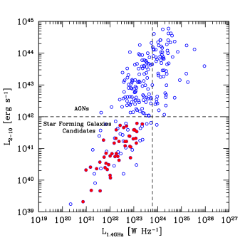
Figure 3: Hard X–ray luminosity versus radio luminosity for all the 257 sources detected both in X-ray and radio, and with measured redshift. The SF galaxy candidate sector is the bottom left identified with dashed lines. Sources above the luminosity values indicated by the dashed lines are classified as AGN, while the lower left corner is populated with a mix of star forming galaxies and low luminosity AGN. Final SFG sources obtained with our full selection procedure are indicated with filled circles.

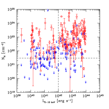
Figure 4: Intrinsic absorption $N_{H}$ versus hard band intrinsic X-ray luminosity for all radio sources with an X-ray counterpart. Error bars refer to 1 $\sigma$. Arrows show 1 $\sigma$ upper limits. The horizontal and vertical dashed lines show the thresholds in intrinsic absorption and hard X-ray luminosity between AGN and SFG, respectively.

We perform the X-ray analysis based on the new 4 Ms data in the CDFS for the sources within 9.5 arcmin of the aimpoint, while we use the E-CDFS data otherwise. Among the 268 radio sources with an X-ray counterpart, 257 ($\sim$ 95$\%$) have a spectroscopic or photometric redshift. Most of the 11 sources without redshift lie on the edge of the optical coverage or near bright stars. Therefore, their redshift estimation is very difficult. We decide to exclude these sources from the analysis. We check a posteriori that including these sources assuming a redshift of 1, which is the average redshift of our sample, does not affect significantly the analysis. The intrinsic X-ray emission of the sources is modeled with a power law with slope $\Gamma$, which is left free only for spectra with more than 170 net counts, while it is frozen to $\Gamma$=1.8 in cases of sources with fewer counts (as in Tozzi et al. 2006). We model the intrinsic absorption with zwabs at the redshift of the source. The local Galactic absorption is modelled with tbabs with a column density fixed to $N_{H}=8.9\times 10^{19}$ cm^-2. We include the redshifted K–shell neutral Fe line modelled as a Gaussian component with zero width at $6.4/(1+z)$ keV. We perform X-ray spectral fits for almost all the sources in our sample, including spectra with a net number of counts as low as 20. The rest–frame, intrinsic X–ray luminosities are computed in the soft and hard band from the best-fit models, after removing the intrinsic absorption. In some cases, the measured intrinsic absorption has a large uncertainty which is accounted for by the statistical error estimated within Xspec. We take into account this uncertainty when measuring the unabsorbed luminosity and associated error. The error on the X-ray luminosity includes also the Poissonian uncertainty in the total net detected counts. Radio luminosities are computed as $L_{1.4GHz}=4\pi d^{2}_{L}S_{1.4GHz}10^{-33}(1+z)^{\alpha_{R}-1}$ W Hz^-1, where $d_{L}$ is the luminosity distance (cm) and $S_{1.4GHz}$ is the flux density ($mJy$), assuming an average value $\alpha_{R}=0.7$ for the radio slope.

In Figure 3 we plot the intrinsic X–ray 2-10 kev (rest frame) luminosity versus the radio luminosity for all 257 sources with X–ray and radio detections with measured redshift. The lower left quadrant with $L_{X}<10^{42}$ erg s^-1 and $L_{R}<5\times 10^{23}$ W Hz^-1 provides a first selection for the star forming galaxy candidates, based on the emitted power (76 sources). We note that there is a large scatter along an apparent correlation between $L_{X}-L_{R}$ across five orders of magnitudes in luminosity. We also note that the upper limit on the X-ray luminosity is much more efficient in classifying star forming galaxies than the threshold on the radio luminosity, since almost all sources screened by radio luminosity are already screened by the X-ray luminosity criterion.

In Figure 4 we plot the intrinsic absorption versus the hard X-ray luminosity for all the radio sources with X-ray counterpart. Typically AGN can be classified in two groups on the basis of their X-ray spectra, absorbed and unabsorbed AGNs, depending whether their intrinsic absorption is above or below the threshold $N_{H}=10^{22}$ cm^-2. In any case, as we discussed, a firm detection of intrinsic absorption indicates that the X-ray emission is powered by a nuclear source. Therefore we flag as AGN all the sources with $N_{H}>3\times 10^{21}$ cm^-2 at least at one $\sigma$ confidence level, as shown in Figures 4. Then we check the presence of the Fe K line, measuring equivalent width of the Gaussian component at $6.4/(1+z)$ keV. A detailed X-ray spectral analysis is important since it allows us to identify as AGN 24 sources of those selected with luminosity below $10^{42}$ erg s^-1, 13 because of the intrinsic absorption and 11 because of the Fe line feature. We also remove from our SFG candidates sample all sources with evident variability in X-ray or radio flux density, rejecting 3 sources in both cases. Optical flux in the R-band is available for the 87% of our sample. The criterion on the X-ray to optical flux ratio, Log F_X/F${}_{opt.}<$ -1, identifies 3 additional AGN. The criterion on the radio slope $\alpha_{R}>$ -0.3 does not have any effect when applied after the other criteria. As a further check we verify that no sources have radio morphology typical of FR I. We show in Table 2 the effect of each single criterion, on the radio sources with X-ray counterpart. We note that the most effective criterion is the X-ray luminosity, and, overall, the use of the selection based only on the X-ray data is strong enough to screen $\sim 98$% of AGN. To summarize, we classify as star forming galaxies 43 sources out of 257 on the basis of X-ray and radio data. The fraction of sources detected in both bands and classified as SFG ($\sim 17$%) is much lower with respect to previous works based on shallower data in the same E–CDFS region (60%, see Rovilos et al. 2007). This is due to our more conservative selection criteria, despite that we do not include IR data.

Table 2: SFG and AGN are the number of galaxies identified as powered by star formation or nuclear activity, respectively, in the sample of 257 sources detected in both bands, according to single selection criteria.

Selection criterion	SFG	AGN
X-ray luminosity	78	179
Column density	131	126
Fe line	229	28
X-ray variability	212	45
FX/Fopt	148	109
All X-ray criteria	47	210
Radio luminosity	172	85
Radio variability	99	15
All radio criteria	164	93

We compare our classification method with that of Padovani et al. (2011) for the 73 sources we have in common. In Papers V, the classification method relies also on optical and IR photometry, and, when available, optical spectroscopy and morphology. Among the sample of star forming galaxy candidates, 6 sources are identified as objects powered by nuclear activity by Padovani et al. (2011). These 6 sources are classified as AGN by criteria or bands not available for all our sample, where additional signatures of nuclear activity may be observed. Specifically, all of them have a $q$ ratio lower than 1.7, the nominal dividing value between SFGs ($q>1.7$) and AGNs ($q<1.7$). We decide to keep these sources in our SF candidate sample, since both X-ray and radio data are still consistent with being powered by star formation only.

4.3 Star forming galaxy candidates with X-ray detection only

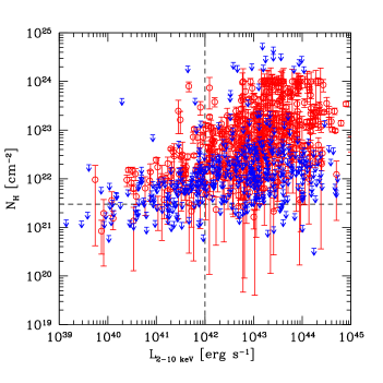
Figure 5: Intrinsic absorption $N_{H}$ versus hard band X-ray luminosity in the sample of X-ray sources with no detection in the radio. Error bars refer to 1 $\sigma$. The horizontal dashed line shows the threshold between AGN and SFG, $N_{H}=3\times 10^{21}$ cm^-2, while the vertical one shows the nominal dividing X-ray power between star forming galaxies and AGN.

Here we check for SFG among the X-ray sources without radio detections. Clearly, only the X-ray criteria can be applied. In the 4 Ms and E–CDFS catalogs there are respectively 564 and 587 sources detected only in the X–ray band. Excluding common detections in the two catalogs in the central part of the field and 10 sources already classified as stars, there are 1074 X–ray extragalactic sources with no radio counterpart in the E–CDFS area. Among them, 899 ($\sim 83$ %) have optical spectroscopic or photometric redshifts. For these sources we can apply the same criteria based on $L_{X}$ and the properties extracted from the spectral analysis, $N_{H}$, the equivalent width of the Fe line and F_X/F_opt. Given the negligible effect of the upper limit on the radio luminosity used in Section 4.1, we notice that these sources are selected with essentially the same criteria as those with a radio counterpart except for radio variability.

The intrinsic absorption of the sample of sources detected only in the X-ray is shown in Figure 5. In the subsample of 899 sources with known redshift, 208 ($\sim$23$\%$) have an X–ray luminosity below $10^{42}$ erg s^-1. It is also evident that lager values of intrinsic absorption becomes common at high luminosity. Applying the criteria based on X-ray hard luminosity, intrinsic absorption, Fe K line presence, variability and the F_X/F_opt. ratio, using the R-band magnitudes from Xue et al. (2011) and Lehmer et al. (2005), we identify 70 SF galaxy candidates. Therefore we add 70 sources classified as SF galaxy candidates, with upper limits in the radio band obtained by measuring flux density in the VLA image at the position of the X-ray source (see Miller et al. 2011). For these sources we use $3\sigma$ radio upper limits at the X-ray position, and we will take them into account in the censored data analysis of the $L_{R}$-$L_{X}$ correlation in section 5.

4.4 Star forming galaxy candidate with radio detection only

In this section we analyze all the radio sources with no X-ray detections in the E-CDFS. In our radio catalog (S/N $>$ 5) we find 705 single sources, excluding multiple components, with radio-only detections. Among them 423 ($\sim$ 60 %) have spectroscopic or photometric redshifts. We evaluate the X-ray upper limits of these sources by performing photometry on the X-ray image after removing all the X-ray detected sources. Then we calculate the conversion factor between the vignetting-corrected count rate and the flux, assuming a simple power law spectrum without intrinsic absorption, and evaluate the luminosity at each radio source position. Due to the impossibility of performing a complete spectral analysis we cannot rely on additional X-ray indicators of nuclear activity such as strong absorption and Fe emission lines. We select as star forming galaxy candidates 117 objects with radio luminosity lower than $5\times 10^{23}$ W Hz^-1 and 3 $\sigma$ upper limit on X-ray luminosity lower than $10^{42}$ erg s^-1. We removed 4 sources showing radio variability and 2 because of the presence of jets. We also checked for consistency with the multiwavelength classification obtained in Paper V for a subsample of these sources. We find a total of 9 SF galaxies in the radio only sample that were classified as AGNs in Paper V. Again we decide to keep these sources. As a further check we stack X-ray images of radio sources in three redshift bins. The stacked signal is null in the hard band, therefore the average hardness ratio (HR) of the radio sources is non measurable but still consistent with a soft spectrum. Since the selection of this sample is weaker than the previous ones, due to the lack of X-ray detections, a further screening should be done with a multiwavelength analysis. Nevertheless, we select a total of 111 SFG candidates with redshifts among the radio only sample, and we will consider them in the correlation analysis.

5 The $L_{R}$-$L_{X}$ correlation for SF galaxies at high redshift

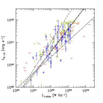
Figure 6: Radio X-ray luminosity relation for all the star forming candidates. The open circles are the radio sources with X-ray counterparts. Error bars refer to 1 $\sigma$. The arrows are the radio and X-ray 1 $\sigma$ upper limits, respectively. The four lines shows Eqs. 1-4. The solid line is the best-fit of the data detected in both bands assuming a slope of unity. The short dashed line is the linear fit of matches without a fixed slope. The dot-short-dashed and dot-long dashed lines are the best fit obtained with censored analysis using also the sources detected only in the X-ray or radio band, respectively, with upper limits in the other band.

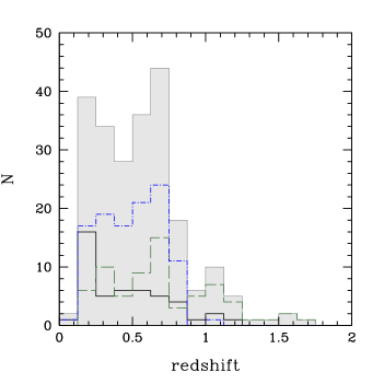
Figure 7: Redshift distribution of star forming galaxy candidates selected in the three samples of sources. The solid line is the histogram of sources detected in both X-ray and radio bands. The dashed line is the histogram of sources detected only in the X-ray band and the dot-dashed line is the histogram of sources detected only in the radio band. The shaded histogram is the distribution of the total sample.

We selected SF galaxy candidates by requiring that both X-ray and radio properties are consistent with being powered by star formation. This is clearly a conservative estimate, since the presence of nuclear emission in one band implies the rejection of the sources, even if, in principle, the emission in the other band may not be contaminated by the nuclear emission. For example, in Paper V, radio quiet AGN have been found consistent with being powered by star formation in the radio band. We do not aim at obtaining a complete census of star formation, therefore we remark that our selection does not allow us to trace directly the cosmic star formation rate.

To investigate the $L_{R}$-$L_{X}$ relation at high redshift we use the sample of 43 star forming galaxies with detections in both bands, together with the 70 sources detected in the X-ray band only and the 111 detected only in the radio. We find a strong correlation (the coefficient of Spearman test is 0.75, with a null hypothesis probability of 6$\times$10^-9) over almost three orders of magnitude for sources detected in both bands.

Assuming a linear relation with the slope fixed to unity, similar to what was done by Ranalli et al. (2003), we find

$$Log(L_{2-10keV})=Log(L_{1.4GHz})+18.60\pm 0.44,$$ (1)

where $L_{2-10keV}$ is in erg s^-1 and $L_{1.4GHz}$ is in W Hz^-1 (see Figure 6, solid line).

If we leave the slope free to vary, we find:

$$Log(L_{2-10keV})=(1.04\pm 0.05)\times Log(L_{1.4GHz})+(17.68\pm 1.15)\,$$ (2)

obtained by performing two least-squares regressions assuming alternatively $L_{2-10keV}$ or $L_{1.4GHz}$ as independent variable, and then using the bisector method (Isobe et al., 1990). This relation is consistent with the fit found fixing the slope to unity (see Figure 6, dashed line). Moreover, it is consistent with the linear relation found for local SF galaxies. We are aware that the relation may not hold for low luminosity galaxies, where the SFR may not be proportional to the HMXB population (Grimm et al., 2003).

We note a large uncertainty in the normalization of this relation (a factor from 3 to 10 assuming a fixed slope or a free slope, respectively, at 1 $\sigma$ level). This uncertainty is largely due to the significant scatter in the observed relation which appears to be larger than that observed for local SF galaxies. The standard deviation of the X-ray luminosity with respect to the average relation is 0.41 dex, as opposed to 0.24 dex found in Ranalli et al. (2003). Since the average 1 $\sigma$ error of our X-ray luminosities is 0.06 dex, we conclude that the scatter is mostly due to an intrinsic component. The scatter can be due to an increasing X-ray emission component proportional to stellar mass and not to the instantaneous SFR, analogous to what has been found in a sample of luminous infrared galaxies by Lehmer et al. (2010).

We now consider the star forming candidates detected only in one band, including the upper limits at 3 sigma in the other band. We use the software for statistical analysis ASURV (Feigelson & Nelson, 1985; Isobe et al., 1986). This tool allows us to perform censored data analysis, including first upper limits in the radio band and then separately the upper limits in X-ray band. The best-fits for the $L_{R}$-$L_{X}$ relation, adding X-ray–only sources or radio-only sources, are, respectively:

$$Log(L_{2-10keV})=(1.22\pm 0.15)\times Log(L_{1.4GHz})+(14.02\pm 3.22)\,$$ (3)

$$Log(L_{2-10keV})=(0.71\pm 0.08)\times Log(L_{1.4GHz})+(24.70\pm 1.74)\,.$$ (4)

In both cases an X-ray/radio correlation is detected at more than 3 sigma confidence level. The fit which includes X-ray–only sources is consistent with a slope equal to 1. On the contrary, the slope found including radio–only sources is inconsistent with unity. This result is similar to that found by Lehmer et al. (2010) for SFR $\gtrsim 0.4M_{\odot}yr^{-1}$, suggesting that the dependence of $L_{X}$ on SFR is not linear. Deeper X-ray data and radio would help to obtain more robust results for our high-redshift galaxies.

For star forming candidates detected in both bands, we also check if there is some evolution with redshift in the relation, by separating low redshift ($z<0.5$) objects from high redshift ($z\geq 0.5$ ) ones. We find that the intercept varies from 18.66 for low redshift sources to 18.47 for high redshift sources, with an uncertainty of 0.4 dex in both cases, therefore showing no evolution. This confirms the claim of Bauer et al. (2002) based on a smaller sample of SF galaxies in the CDFN. In Figure 7 we show the redshift distribution of our star forming galaxy candidates. It shows that most of SF galaxies are distributed up to redshift 1, with a small fraction ($\sim$15$\%$) at higher redshift. The average redshift is $<z>\sim 0.5$, while $<z>_{matches}\sim 0.4$ for the sources detected in both bands. While AGNs are distributed up to high redshifts, star forming galaxies can be observed in the radio and X-ray with current data only up to redshift 1.5-2, as discussed in Section 6.2.

To summarize, we do find a clear correlation between the X-ray and radio luminosity for star forming galaxies. This result is robust when we include upper limits in the X-ray or radio bands in a censored data analysis, at variance with the claim by Barger et al. (2007). However, the observed correlation at high redshift appears to have a large intrinsic scatter, and its slope is still unclear. Both these features may be due to an increasing X-ray contribution proportional to the total stellar mass and unrelated to the instantaneous SFR. In the following sections, we make use of the best-fit linear relation (Eq. 1) to estimate the star formation rate of our sources.

6 Star Formation Rate

To derive the average $L_{X}$-SFR relation in the selected sample of star-forming galaxies, we use the measured $L_{X}$-$L_{R}$ relation and the local-calibrated SFR-$L_{R}$. We adopt the calibration between $L_{R}$ and SFR found by Bell (2003):

$$SFR=5.52\times 10^{-22}L_{1.4GHz}M_{\odot}/yr\,,$$ (5)

where $L_{1.4GHz}$ is in W Hz^-1. Assuming Eq. (1) and substituting into Eq. (5) we find:

$$SFR=(1.40\pm 0.32)\times\frac{L_{2-10keV}}{10^{40}}M_{\odot}/yr\,,$$ (6)

where $L_{2-10keV}$ is in erg s^-1. This relation is a factor of 2 lower than that obtained by Persic & Rephaeli (2007) for their low redshift sample, where they found a factor 2.6$\times 10^{-40}$ between the SFR and the X-ray hard luminosity, but still consistent within the uncertainty. We list our estimated SFR in Table 8 along with the X-ray and radio luminosity.

In Figure 8 we show the distribution of the estimated SF rates in our sample derived directly from their radio luminosity. Most of SFGs (60-70 $\%$) have star formation rate lower than 30 $M_{\odot}yr^{-1}$. About 20% of galaxies have SFR which exceeds $50M_{\odot}yr^{-1}$. This implies a mix of different type of SFG, from normal spirals to strong starburst, as we discuss in the next section.

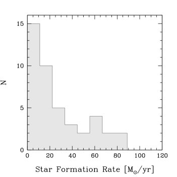
Figure 8: Star formation rate distribution SF galaxy candidates with X-ray and radio detection. The SFR is evaluated using the SFR-L_R relation.

6.1 Comparison with models

We use chemical evolution models to predict the typical star formation rate as a function of redshift in different galaxy types. In particular, we took into account the predictions from a model devised for the Milky Way (Cescutti et al., 2007). This model is based on the two–infall model of Chiappini et al. (1997), which assumes that the Milky Way formed in two major steps by means of gas accretion. The first gas accretion episode formed the halo and the thick disc on a timescale not exceeding 2 Gyr, whereas the second episode formed the thin disc on a much longer timescale (e.g., 8 Gyr at the solar ring). This model accurately reproduces many properties of the Galactic disc and therefore it can be used as an example of a normal spiral. The star formation rate is obtained by assuming a dependence on the surface gas density $\Sigma_{gas}$ as suggested by Kennicutt (1998); in particular, a dependence $SFR\propto\Sigma_{gas}^{k}$ with $k=1.5$ and a threshold $\Sigma_{gas}=7M_{\odot}pc^{-2}$ in the gas density are assumed. The total star formation rate is the sum of that occurring in the bulge and that occurring in the thin disc. The model for the bulge of the Milky Way assumes that the SFR was much more intense and faster than in the discs. The model also accounts for a varying SFR decreasing with galactocentric distance. We assume that the star formation started at redshift $z_{f}=10$. A similar model has been computed for the bulge and the disc of M31 which has a mass roughly two times higher than the Milky Way. These models both reproduce the main properties of the bulges of the Milky Way and M31 (Ballero et al. 2007a, 2007b) . In Figure 9 we show the total predicted SFR (thick lines) compared with our measured star formation rates as a function of redshift. We note that for $z<1.5$ only the disc component is visible since the star formation in the bulge ended at high redshift. The disc SFR for the Milky Way and M31 reaches values comparable with the lowest found in our analysis, showing that the majority of our star forming galaxies form stars ten times more efficiently than Milky Way-like objects, up to a level comparable to the strong starburst M82 (horizontal stripe). Obviously this is due to the flux limit of our survey which allows us to detect Milky Way-like only for $z<0.3$. We also note that a significant fraction of our galaxies reach values higher that that of M82 and comparable with the model predictions for formation of the Galactic bulge. This is shown in Figure 9 by the thin lines, which have been obtained by setting a formation time of $z_{f}=$1.5. Although this is not realistic, since in true bulges are generally old, it suggests that our star forming galaxies span a wide range of starburst, from normal discs to strong burst typical of bulge formation.

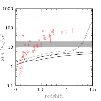
Figure 9: SFR evaluated in our sample of galaxies detected in both X-ray and radio. The lines represent the different models compared to the data. The solid and dashed thick lines represent respectively the SFR in the Milky Way and M31, if we assume that the star formation started at z${}_{f}=10$. The thin curves are the same galaxies in the case of a formation time of z_f=1.5. The horizontal stripe represents the observed SFR in the typical local starburst galaxy M82.

6.2 Prospects for star forming galaxy survey

Due to the tight relation observed for the radio and X-ray emission of star forming galaxies, we expect to see all the sources powered by star formation in both bands, when an adequate sensitivity limit is reached. Assuming the linear correlations between the SFR and the radio and X-ray luminosity, as evaluated by Bell (2003) and our Eq. 6, respectively, we compute a minimum detectable SFR at any given redshift. Taking the lowest limit in the X-ray and radio CDFS surveys, we plot in Figure 10 the minimum star formation rate that we can detect in these two surveys. We assumed a 10% accuracy in both cases in the relation between luminosity and star formation rate.

If we refer to M82 as a typical starburst galaxy in the local universe, we immediately see the redshift range that we are actually exploring. M82 has a SFR of $10-20M_{\odot}yr^{-1}$, corresponding to more than 10 times that in the Milky Way at the present time (e.g., Doane & Mathews 1993). A similar starburst galaxy can be seen up to $z\sim 0.2$ in the X-ray E-CDFS, and up to $z\sim 0.6$ with the radio VLA and in the 4 Ms data of the CDFS (note that this holds only for the part of the field which reaches the most sensitive levels). As a consequence, lower values, typical of normal galaxies ($1-10M_{\odot}yr^{-1}$) can be seen only at moderate redshift $z<0.4$. In the strong starburst regime ($10-100M_{\odot}yr^{-1}$) it is possible to reach redshift as high as $z\sim 1.5$. At larger redshift, only the bright end of the SFG population is observable, i.e. starburst galaxies with extremely large SF rates $>100M_{\odot}yr^{-1}$. A typical example of the latter population is Arp220, a nearby system in final stages of galaxy merger with a powerful burst of star formation at each of the nuclei and close to its peak in activity, which results in strong radio, FIR and X-ray emission. Models of the embedded starburst suggest a SFR$=340-10^{3}$ $M_{\odot}yr^{-1}$, depending on the assumed star formation tracer (Baan, 2007), observable in our surveys up to $z\gtrsim 2$. To explore the range $>100M_{\odot}yr^{-1}$ up to $z=2$ is necessary to reach a factor $\sim 2.5$ higher sensitivity (corresponding to the ideal 10 Ms goal for the CDFS in the X-ray band). At the same time we would reach a complete census of strong starbursts (from M82 on) up to redshift 1.

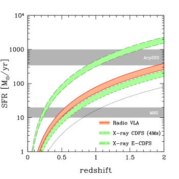
Figure 10: Minimum measurable star formation rate as a function of redshift in the X-ray CDFS 4Ms, E-CDFS and radio surveys. The SFR value corresponds to the hard band flux limit and to the 1.4 GHz flux density limit in the X-ray and radio band respectively, therefore it cannot be applied to the entire E-CDFS field. We assume the Bell (2003) correlation and Eq. 6 between the SFR and the radio and X-ray luminosity respectively, with an average uncertainty of 10%. The horizontal stripes represent the observed SFR in the typical local starburst galaxies M82 and Arp220. The dotted line shows the limit that a 10Ms Chandra exposure in the CDFS would be able to reach.

7 Conclusions

Both radio and X-ray emission can be a clue to ongoing star formation activity with the advantage of not being absorbed by dust. In particular, the collective emission in the radio band is produced by H II regions and supernovae, while in the X-ray band originates from the HMXBs and $\sim 1$ keV gas heated by stellar winds. In the assumption that both bands always act as a calorimeter for the emission from massive, short-lived stars, we expect to observe a well defined correlation between X-ray and radio luminosity up to high redshift.

In this paper we aim at exploring such a correlation using the deep X-ray and radio data in the E–CDFS area (Lehmer et al. 2005; Xue et al. 2011; Miller et al. 2011) . The starting sample includes $\sim 1300$ X-ray sources and $\sim 900$ radio sources. Many of them have an identified optical or IR counterpart (Xue et al. 2011; Bonzini et al. in preparation). A spectroscopic or photometric redshift is known for 85% and 73% of the X-ray and radio sources, respectively. First, we identify all the sources which are detected in both bands. Then, on the basis of the radio data and of a detailed X-ray spectroscopy we select a sample of star forming galaxy candidates. This allows us to investigate the correlation between the radio and X-ray luminosity, and to extend the measure of the star formation rate for our sources over a large redshift range up to 1.5. Our results are summarized as follows:

• Among the 268 sources with both radio and X–ray detections, most of which have spectroscopic or photometric redshifts, 43 ($\sim$16%) are consistent with being powered by star formation processes in both bands. The main criteria are the X–ray and radio luminosity, the intrinsic absorption, the presence of the Fe emission line, and the time variability. Among the sources detected only in the X-ray or the radio band, we select 70 and 111 star forming candidates, respectively. Their classification, though, being based on a smaller number of criteria, is more uncertain;

• We find that for the sources detected in both bands the $L_{X}-L_{R}$ relation is well fitted with a slope close to 1: $Log(L_{2-10keV})=(1.04\pm 0.05)\times Log(L_{1.4GHz})+(17.68\pm 1.15)$. The fit which includes X-ray upper limits, treated with censored data analysis, is consistent with the previous relation. On the contrary, the inclusion of upper limits in the radio band leads to a flatter relation, which is suggesting of a non linear dependence of $L_{X}$ on instantaneous star formation. Deeper data are needed to obtain more robust results at high redshift;

• Assuming a linear slope in the $L_{X}-L_{R}$ relation and splitting our sample in low and high redshift bins, we find no evolution in redshift;

• We find that the $L_{X}-L_{R}$ relation shows a significant scatter. We estimate its intrinsic component to be 0.4 dex, possibly due to a contribution to X-ray luminosity unrelated to the instantaneous SFR;

• Finally we compute relation between SFR and X-ray luminosity in the 2-10 keV band: $SFR=(1.40\pm 0.32)\times L_{2-10keV}$ $10^{-40}$ M_⊙/yr. Most of the sources ( 60$\%$) have a SFR lower than 30 M_⊙/yr. A small number sources have a SFR higher than 50-60 M_⊙/yr. The comparison of these data with models of chemical evolution allows us to explore the nature of the SFG galaxies. The SFRs we measure in our deep narrow survey span a wide range from normal spirals like the Milky Way or M31, to starburst like M82, up to strong starburst typical of bulges and spheroids in formation.

The strong correlation of SFR with the hard X-ray luminosity in our high-z galaxy sample shows that X-ray surveys can provide a powerful and independent tool in measuring the instantaneous SFR in distant galaxies. However, our data also indicates that the complex physics behind the X-ray and radio emission associated to star formation, may introduce significant scatter between $L_{X}$ and SFR.

Table 3: X–ray spectral analysis results of sources with radio counterparts in the CDFS area. X ID are from Xue et al. (2011); z is the spectroscopic or photometric redshift; $\Gamma$ is the slope of the intrinsic X-ray emission modelled with a power law; $N_{H}$ is the column density; $L_{0.5-2keV}$ and $L_{2-10keV}$ are the luminosities in the soft and X-ray band respectively.

Xue X ID	z	$\Gamma$	$N_{H}$ ($10^{22}$ cm-2)	$L_{0.5-2keV}$ erg s-1	$L_{2-10keV}$ erg s-1
16	1.94	2.1 $\pm$ 0.4	$<$ 2.27	$1.03\pm 0.19\times 10^{43}$	$1.76\pm 0.32\times 10^{43}$
18	2.14	1.2 $\pm$ 0.7	$64^{+37}_{-20}$	$1.04\pm 0.19\times 10^{43}$	$5.88\pm 1.09\times 10^{43}$
23	0.18	1.8	$<$ 1.89	$1.82\pm 0.62\times 10^{40}$	$3.26\pm 1.11\times 10^{40}$
27	4.39	1.8	$80^{+31}_{-24}$	$2.55\pm 0.67\times 10^{43}$	$2.32\pm 0.61\times 10^{44}$
29	2.26	1.8	$32^{+41}_{-19}$	$7.75\pm 2.88\times 10^{42}$	$2.24\pm 0.83\times 10^{43}$
31	0.86	1.8	$6.7^{+5.9}_{-3.2}$	$2.41\pm 0.94\times 10^{42}$	$4.40\pm 1.71\times 10^{42}$
34	2.94	1.7 $\pm$ 0.4	$30^{+32}_{-16}$	$4.14\pm 0.59\times 10^{43}$	$1.74\pm 0.25\times 10^{44}$
39	2.81	1.0 $\pm$ 0.5	$<$ 8.8	$3.03\pm 0.44\times 10^{42}$	$2.83\pm 0.41\times 10^{43}$
45	0.74	1.8	$<$ 0.1	$1.19\pm 0.16\times 10^{41}$	$2.22\pm 0.31\times 10^{41}$
48	3.20	1.1 $\pm$ 0.3	$23^{+36}_{-14}$	$4.93\pm 0.75\times 10^{42}$	$4.64\pm 0.70\times 10^{43}$
57	0.56	1.5 $\pm$ 0.3	$3.8^{+2.4}_{-1.8}$	$7.88\pm 1.10\times 10^{41}$	$2.03\pm 0.28\times 10^{42}$
63	0.67	1.4 $\pm$ 0.1	$<$ 0.38	$1.20\pm 0.11\times 10^{42}$	$3.21\pm 0.29\times 10^{42}$
67	1.99	1.6 $\pm$ 0.1	$5.0^{+0.7}_{-0.6}$	$5.14\pm 0.13\times 10^{43}$	$1.62\pm 0.04\times 10^{44}$
81	0.98	1.8	$<$ 2.13	$2.18\pm 1.66\times 10^{41}$	$3.83\pm 2.92\times 10^{41}$
83	1.50	1.0 $\pm$ 0.2	$14^{+1}_{-1}$	$1.76\pm 0.04\times 10^{43}$	$1.13\pm 0.03\times 10^{44}$
97	0.57	1.7 $\pm$ 0.1	$6.7^{+0.6}_{-0.6}$	$6.44\pm 0.20\times 10^{42}$	$1.22\pm 0.04\times 10^{43}$
109	0.72	1.0 $\pm$ 0.7	$15^{+6}_{-3}$	$2.03\pm 0.24\times 10^{42}$	$1.09\pm 0.13\times 10^{43}$
114	1.00	1.8	$<$ 0.0	$7.30\pm 1.09\times 10^{40}$	$1.29\pm 0.19\times 10^{41}$
115	1.07	1.8	$9.1^{+11.7}_{-7.0}$	$7.32\pm 1.03\times 10^{41}$	$1.33\pm 0.19\times 10^{42}$
120	1.02	1.8	$<$ 0.01	$1.37\pm 0.52\times 10^{41}$	$3.44\pm 1.30\times 10^{41}$
127	0.77	1.8	$<$ 0.01	$1.06\pm 0.30\times 10^{42}$	$1.73\pm 0.48\times 10^{42}$
131	0.03	1.8	$14^{+27}_{-10}$	$1.30\pm 0.29\times 10^{39}$	$2.36\pm 0.52\times 10^{39}$
132	3.53	1.8	$13^{+9}_{-8}$	$4.63\pm 1.27\times 10^{42}$	$2.36\pm 0.65\times 10^{43}$
139	1.00	1.0 $\pm$ 0.5	$1.8^{+1.2}_{-0.9}$	$1.38\pm 0.19\times 10^{42}$	$7.91\pm 1.06\times 10^{42}$
140	0.31	1.8	$<$ 0.09	$3.78\pm 0.52\times 10^{40}$	$1.06\pm 0.15\times 10^{41}$
141	0.54	1.9	$<$ 0.01	$4.79\pm 0.03\times 10^{43}$	$6.86\pm 0.04\times 10^{43}$
151	0.73	2.5 $\pm$ 0.2	$<$ 0.07	$1.71\pm 0.19\times 10^{42}$	$1.04\pm 0.12\times 10^{42}$
152	0.74	1.8	$<$ 0.81	$1.27\pm 0.17\times 10^{41}$	$2.06\pm 0.28\times 10^{41}$
154	0.08	1.8	$<$ 0.11	$1.35\pm 0.58\times 10^{39}$	$2.12\pm 0.91\times 10^{39}$
156	1.16	1.8	$2.9^{+1.5}_{-1.2}$	$1.46\pm 0.20\times 10^{42}$	$2.89\pm 0.39\times 10^{42}$
160	1.26	1.8 $\pm$ 0.0	$0.94^{+0.15}_{-0.15}$	$4.66\pm 0.08\times 10^{43}$	$8.70\pm 0.14\times 10^{43}$
161	0.65	1.8	$<$ 5.26	$2.32\pm 1.59\times 10^{40}$	$9.45\pm 6.45\times 10^{40}$
163	1.61	1.8	$<$ 0.78	$9.62\pm 2.84\times 10^{41}$	$2.25\pm 0.66\times 10^{42}$
166	1.62	1.7 $\pm$ 0.0	$<$ 0.12	$5.11\pm 0.08\times 10^{43}$	$1.31\pm 0.02\times 10^{44}$
164	0.42	1.8	$<$ 0.35	$2.89\pm 1.15\times 10^{40}$	$5.92\pm 2.36\times 10^{40}$
168	0.18	1.4 $\pm$ 0.1	$<$ 0.07	$9.34\pm 0.55\times 10^{40}$	$2.81\pm 0.16\times 10^{41}$
174	0.58	1.8	$1.1^{+1.6}_{-0.9}$	$1.06\pm 0.42\times 10^{41}$	$1.81\pm 0.72\times 10^{41}$
180	1.03	1.4 $\pm$ 0.1	$2.6^{+0.8}_{-0.8}$	$2.82\pm 0.14\times 10^{42}$	$8.86\pm 0.44\times 10^{42}$
193	0.61	1.6 $\pm$ 0.1	$2.2^{+0.3}_{-0.3}$	$6.43\pm 0.15\times 10^{42}$	$1.43\pm 0.03\times 10^{43}$
197	2.68	1.6 $\pm$ 0.3	$21^{+18}_{-14}$	$1.46\pm 0.21\times 10^{43}$	$6.32\pm 0.92\times 10^{43}$
198	0.74	1.0 $\pm$ 0.5	$18^{+7}_{-3}$	$1.48\pm 0.12\times 10^{42}$	$8.15\pm 0.65\times 10^{42}$
202	2.08	1.8	$5.5^{+4.8}_{-3.4}$	$1.55\pm 0.37\times 10^{42}$	$4.11\pm 0.99\times 10^{42}$
217	0.24	1.8	$0.65^{+0.27}_{-0.23}$	$4.87\pm 0.60\times 10^{40}$	$8.03\pm 1.00\times 10^{40}$
226	1.41	1.8	$33^{+46}_{-21}$	$1.25\pm 0.47\times 10^{42}$	$3.21\pm 1.22\times 10^{42}$
228	0.66	1.8	$<$ 0.09	$1.41\pm 0.23\times 10^{41}$	$3.85\pm 0.62\times 10^{41}$
229	1.32	2.0 $\pm$ 0.0	$<$ 0.09	$1.02\pm 0.02\times 10^{44}$	$1.55\pm 0.02\times 10^{44}$
241	0.57	1.8 $\pm$ 0.0	$<$ 0.02	$5.13\pm 0.10\times 10^{42}$	$7.49\pm 0.15\times 10^{42}$
243	1.10	1.6 $\pm$ 0.1	$19^{+2}_{-2}$	$2.87\pm 0.08\times 10^{43}$	$7.44\pm 0.20\times 10^{43}$
244	2.28	1.8	$<$ 2.11	$5.32\pm 0.79\times 10^{41}$	$1.53\pm 0.23\times 10^{42}$
249	0.12	1.8	$<$ 0.65	$3.02\pm 0.81\times 10^{39}$	$4.74\pm 1.27\times 10^{39}$
250	0.73	1.8	$<$ 0.03	$3.42\pm 0.46\times 10^{41}$	$5.51\pm 0.75\times 10^{41}$
251	0.67	1.8	$<$ 0.01	$1.53\pm 0.43\times 10^{42}$	$2.55\pm 0.72\times 10^{42}$
257	1.54	1.0 $\pm$ 0.3	$28^{+2}_{8}$	$6.75\pm 0.29\times 10^{42}$	$4.49\pm 0.19\times 10^{43}$
262	3.66	1.0 $\pm$ 0.3	$41^{+14}_{-9}$	$3.53\pm 0.31\times 10^{42}$	$4.85\pm 0.43\times 10^{43}$
271	0.76	1.8	$<$ 0.01	$1.92\pm 0.65\times 10^{41}$	$3.41\pm 1.12\times 10^{41}$
273	1.98	1.8	$6.9^{+8.1}_{-5.9}$	$1.38\pm 0.20\times 10^{42}$	$3.53\pm 0.50\times 10^{42}$
274	0.23	1.8	$<$ 0.10	$3.23\pm 0.62\times 10^{40}$	$7.74\pm 1.48\times 10^{40}$
279	1.22	1.8	$<$ 0.10	$9.49\pm 4.74\times 10^{40}$	$2.64\pm 1.32\times 10^{41}$
287	0.68	1.8	$<$ 0.95	$1.02\pm 0.47\times 10^{41}$	$1.64\pm 0.76\times 10^{41}$

Table 4: continued

Xue X ID	z	$\Gamma$	$N_{H}$ ($10^{22}$ cm-2)	$L_{0.5-2keV}$ erg s-1	$L_{2-10keV}$ erg s-1
289	0.67	1.8	$<$ 0.32	$6.50\pm 2.89\times 10^{40}$	$1.19\pm 0.53\times 10^{41}$
290	2.83	1.5 $\pm$ 0.3	$63^{+43}_{-33}$	$1.21\pm 0.13\times 10^{43}$	$6.42\pm 0.69\times 10^{43}$
292	0.52	1.8	$<$ 0.06	$1.00\pm 0.24\times 10^{41}$	$1.76\pm 0.42\times 10^{41}$
299	2.12	1.8	$<$ 3.56	$9.07\pm 1.22\times 10^{41}$	$2.91\pm 0.39\times 10^{42}$
300	0.20	1.8	$0.37^{+0.37}_{-0.26}$	$2.29\pm 0.62\times 10^{40}$	$3.68\pm 1.00\times 10^{40}$
305	2.62	1.8	$2.9^{+3.0}_{-2.5}$	$3.42\pm 0.51\times 10^{42}$	$1.16\pm 0.17\times 10^{43}$
311	0.74	1.8	$<$ 0.36	$1.69\pm 0.31\times 10^{41}$	$5.06\pm 0.92\times 10^{41}$
314	1.64	1.8	$<$ 1.68	$1.33\pm 0.43\times 10^{42}$	$3.74\pm 1.22\times 10^{42}$
316	0.66	1.8	$<$ 1.82	$5.08\pm 0.65\times 10^{40}$	$1.13\pm 0.14\times 10^{41}$
321	1.03	1.8	$305^{+162}_{-115}$	$1.75\pm 0.78\times 10^{43}$	$3.15\pm 1.41\times 10^{43}$
322	0.58	1.8	$<$ 0.85	$1.04\pm 0.18\times 10^{41}$	$1.63\pm 0.28\times 10^{41}$
324	0.12	1.8	$<$ 1.95	$1.75\pm 0.55\times 10^{40}$	$3.41\pm 1.07\times 10^{40}$
327	0.53	1.7 $\pm$ 0.1	$<$ 0.06	$1.81\pm 0.06\times 10^{42}$	$3.43\pm 0.12\times 10^{42}$
329	1.05	1.0 $\pm$ 1.0	$12^{+141}_{-5}$	$1.29\pm 0.27\times 10^{42}$	$7.85\pm 1.61\times 10^{42}$
330	0.58	1.8	$0.96^{+0.89}_{-0.73}$	$1.46\pm 0.55\times 10^{41}$	$2.72\pm 1.02\times 10^{41}$
343	1.09	2.3 $\pm$ 0.5	$48^{+28}_{-26}$	$2.49\pm 0.35\times 10^{43}$	$2.33\pm 0.32\times 10^{43}$
344	1.62	1.9 $\pm$ 0.1	$0.33^{+0.34}_{-0.31}$	$2.85\pm 0.08\times 10^{43}$	$5.59\pm 0.15\times 10^{43}$
348	2.54	1.8	$<$ 2.03	$1.35\pm 0.45\times 10^{42}$	$4.31\pm 1.44\times 10^{42}$
349	0.90	1.8	$<$ 0.32	$1.71\pm 0.29\times 10^{41}$	$3.95\pm 0.66\times 10^{41}$
367	1.03	2.3 $\pm$ 0.0	$<$ 0.01	$1.10\pm 0.01\times 10^{44}$	$9.44\pm 0.11\times 10^{43}$
383	1.10	1.8	$<$ 0.60	$1.61\pm 0.56\times 10^{41}$	$6.12\pm 2.11\times 10^{41}$
385	0.25	1.8	$<$ 1.34	$1.23\pm 0.21\times 10^{40}$	$2.74\pm 0.46\times 10^{40}$
387	0.21	1.8	$<$ 0.10	$4.49\pm 1.56\times 10^{40}$	$7.04\pm 2.44\times 10^{40}$
391	0.74	1.8 $\pm$ 0.1	$<$ 0.12	$6.42\pm 0.51\times 10^{41}$	$1.05\pm 0.08\times 10^{42}$
393	0.22	1.7 $\pm$ 0.1	$0.27^{+0.14}_{-0.07}$	$8.31\pm 0.46\times 10^{40}$	$1.64\pm 0.09\times 10^{41}$
396	0.62	1.5 $\pm$ 0.1	$<$ 0.11	$2.34\pm 0.11\times 10^{42}$	$5.99\pm 0.28\times 10^{42}$
407	0.64	1.8	$0.71^{+0.71}_{-0.56}$	$3.52\pm 0.59\times 10^{41}$	$6.13\pm 1.03\times 10^{41}$
413	0.08	2.7 $\pm$ 0.1	$<$ 0.01	$1.10\pm 0.06\times 10^{40}$	$4.67\pm 0.26\times 10^{39}$
418	0.08	2.1 $\pm$ 0.1	$<$ 0.01	$8.51\pm 0.52\times 10^{39}$	$8.30\pm 0.51\times 10^{39}$
420	0.96	2.0 $\pm$ 0.1	$<$ 0.06	$5.65\pm 0.19\times 10^{42}$	$8.09\pm 0.27\times 10^{42}$
429	1.04	1.0 $\pm$ 2.9	$<$ 0.10	$3.87\pm 0.66\times 10^{41}$	$3.05\pm 0.51\times 10^{42}$
435	2.22	1.8	$<$ 0.38	$1.72\pm 0.32\times 10^{42}$	$4.82\pm 0.89\times 10^{42}$
436	1.61	1.8	$302^{+268}_{-141}$	$1.36\pm 0.63\times 10^{43}$	$3.03\pm 1.40\times 10^{43}$
453	0.67	1.8	$<$ 0.16	$1.38\pm 0.46\times 10^{41}$	$2.46\pm 0.82\times 10^{41}$
460	3.62	1.8	$14^{+67}_{-14}$	$2.02\pm 0.64\times 10^{42}$	$1.18\pm 0.37\times 10^{43}$
467	1.38	1.8	$12^{+29}_{-11}$	$4.79\pm 3.20\times 10^{41}$	$1.12\pm 0.75\times 10^{42}$
469	3.00	1.7 $\pm$ 0.4	$27^{+22}_{-13}$	$1.58\pm 0.28\times 10^{43}$	$6.73\pm 1.18\times 10^{43}$
473	0.66	2.0 $\pm$ 0.1	$3.7^{+0.5}_{-0.4}$	$2.97\pm 0.09\times 10^{43}$	$3.28\pm 0.10\times 10^{43}$
474	1.97	1.8	$<$ 9.1	$6.91\pm 1.27\times 10^{41}$	$2.61\pm 0.48\times 10^{42}$
476	1.11	1.8	$<$ 1.57	$1.78\pm 0.92\times 10^{41}$	$3.29\pm 1.70\times 10^{41}$
483	0.04	1.8	$<$ 0.15	$4.93\pm 0.79\times 10^{38}$	$7.73\pm 1.24\times 10^{38}$
490	2.58	1.8	$61^{+35}_{-18}$	$7.45\pm 1.35\times 10^{42}$	$2.81\pm 0.51\times 10^{43}$
500	0.55	1.8	$<$ 0.14	$1.38\pm 0.21\times 10^{41}$	$2.43\pm 0.38\times 10^{41}$
499	1.61	1.6 $\pm$ 0.1	$<$ 1.45	$2.22\pm 0.19\times 10^{42}$	$7.46\pm 0.65\times 10^{42}$
510	0.52	1.8	$<$ 1.01	$7.03\pm 2.31\times 10^{40}$	$1.69\pm 0.55\times 10^{41}$
507	0.13	1.8	$<$ 0.50	$5.56\pm 2.50\times 10^{39}$	$2.32\pm 1.05\times 10^{40}$
517	1.62	1.8	$<$ 1.90	$4.20\pm 1.64\times 10^{41}$	$1.20\pm 0.47\times 10^{42}$
518	1.60	2.1 $\pm$ 0.0	$2.0^{+0.2}_{-0.2}$	$1.23\pm 0.02\times 10^{44}$	$1.75\pm 0.03\times 10^{44}$
519	2.44	1.8	$33^{+20}_{-15}$	$5.86\pm 2.62\times 10^{42}$	$1.80\pm 0.80\times 10^{43}$
521	3.42	1.8	$<$ 29.3	$2.07\pm 0.28\times 10^{42}$	$9.97\pm 1.37\times 10^{42}$
530	0.74	1.8	$<$ 0.28	$1.00\pm 0.15\times 10^{41}$	$2.09\pm 0.31\times 10^{41}$
531	0.24	1.8	$<$ 1.56	$7.49\pm 2.42\times 10^{39}$	$1.18\pm 0.38\times 10^{40}$
533	0.30	1.5 $\pm$ 0.1	$3.1^{+0.2}_{-0.2}$	$4.93\pm 0.08\times 10^{42}$	$1.23\pm 0.02\times 10^{43}$
542	0.69	1.8	$1.6^{+2.0}_{-1.3}$	$2.39\pm 0.84\times 10^{41}$	$4.30\pm 1.52\times 10^{41}$
546	3.06	1.5 $\pm$ 0.1	$42^{+5}_{-5}$	$5.00\pm 0.16\times 10^{43}$	$2.81\pm 0.09\times 10^{44}$
556	0.62	1.0 $\pm$ 0.2	$2.3^{+0.4}_{-0.2}$	$1.71\pm 0.07\times 10^{42}$	$9.13\pm 0.38\times 10^{42}$
566	0.15	1.8	$<$ 0.15	$2.04\pm 0.73\times 10^{40}$	$5.53\pm 1.97\times 10^{40}$
569	0.66	1.8	$0.80^{+0.69}_{-0.53}$	$8.37\pm 2.03\times 10^{41}$	$1.35\pm 0.33\times 10^{42}$
582	0.28	2.8 $\pm$ 0.8	$<$ 0.28	$4.48\pm 0.44\times 10^{40}$	$1.60\pm 0.16\times 10^{40}$
590	0.41	2.0 $\pm$ 0.2	$<$ 0.11	$1.70\pm 0.15\times 10^{41}$	$2.14\pm 0.19\times 10^{41}$
595	0.71	1.8	$<$ 0.40	$1.78\pm 0.75\times 10^{41}$	$3.82\pm 1.61\times 10^{41}$
596	0.21	1.8	$<$ 0.14	$6.24\pm 2.00\times 10^{39}$	$1.20\pm 0.38\times 10^{40}$

Table 5: continued

Xue X ID	z	$\Gamma$	$N_{H}$ ($10^{22}$ cm-2)	$L_{0.5-2keV}$ erg s-1	$L_{2-10keV}$ erg s-1
597	0.46	1.8	$<$ 0.08	$6.67\pm 0.76\times 10^{40}$	$1.20\pm 0.14\times 10^{41}$
598	0.44	1.8	$<$ 0.18	$4.44\pm 0.61\times 10^{40}$	$6.96\pm 0.95\times 10^{40}$
609	0.10	1.8	$<$ 0.07	$8.63\pm 0.93\times 10^{39}$	$2.08\pm 0.22\times 10^{40}$
612	1.99	1.8	$44^{+19}_{-17}$	$6.54\pm 3.72\times 10^{42}$	$1.83\pm 1.04\times 10^{43}$
617	1.10	1.8	$6.5^{+2.4}_{-2.1}$	$5.27\pm 0.98\times 10^{41}$	$1.01\pm 0.19\times 10^{42}$
623	0.73	1.8	$<$ 0.40	$3.83\pm 0.96\times 10^{41}$	$6.15\pm 1.54\times 10^{41}$
626	0.98	1.7 $\pm$ 0.0	$1.8^{+0.1}_{-0.1}$	$6.73\pm 0.08\times 10^{43}$	$1.28\pm 0.01\times 10^{44}$
629	0.67	1.6 $\pm$ 0.1	$2.1^{+0.6}_{-0.5}$	$1.89\pm 0.11\times 10^{42}$	$4.16\pm 0.24\times 10^{42}$
631	1.12	1.8	$<$ 0.89	$3.26\pm 0.41\times 10^{41}$	$6.49\pm 0.81\times 10^{41}$
634	0.55	1.0 $\pm$ 0.8	$4.1^{+2.9}_{-1.3}$	$7.00\pm 1.00\times 10^{41}$	$3.83\pm 0.55\times 10^{42}$
638	0.34	1.8	$<$ 0.09	$3.51\pm 0.84\times 10^{40}$	$5.77\pm 1.38\times 10^{40}$
644	0.97	1.8	$<$ 0.72	$1.41\pm 0.32\times 10^{42}$	$2.48\pm 0.55\times 10^{42}$
652	1.02	2.3 $\pm$ 0.3	$1.5^{+1.4}_{-0.9}$	$5.12\pm 0.56\times 10^{42}$	$4.77\pm 0.52\times 10^{42}$
654	0.53	1.8	$<$ 0.30	$9.49\pm 3.60\times 10^{40}$	$1.49\pm 0.56\times 10^{41}$
656	1.37	1.8	$16^{+11}_{-7}$	$1.80\pm 0.96\times 10^{42}$	$3.64\pm 1.95\times 10^{42}$
658	0.98	1.7 $\pm$ 0.4	$16^{+1}_{8}$	$4.33\pm 0.98\times 10^{42}$	$8.63\pm 1.95\times 10^{42}$
671	0.37	1.8	$<$ 0.28	$8.50\pm 2.65\times 10^{40}$	$1.47\pm 0.46\times 10^{41}$
681	0.73	1.8 $\pm$ 0.1	$<$ 0.04	$6.74\pm 0.20\times 10^{42}$	$1.03\pm 0.03\times 10^{43}$
682	1.15	1.8	$1.8^{+4.2}_{-1.8}$	$6.49\pm 0.76\times 10^{41}$	$1.33\pm 0.16\times 10^{42}$
683	1.20	2.0 $\pm$ 0.1	$17^{+2}_{-1}$	$4.07\pm 0.16\times 10^{43}$	$6.13\pm 0.25\times 10^{43}$
695	0.62	1.7 $\pm$ 0.1	$<$ 0.04	$2.10\pm 0.09\times 10^{42}$	$4.09\pm 0.17\times 10^{42}$
698	3.10	1.8 $\pm$ 0.1	$2.9^{+1.1}_{-0.9}$	$8.64\pm 0.23\times 10^{43}$	$3.55\pm 0.09\times 10^{44}$
700	3.69	1.8 $\pm$ 0.2	$3.5^{+6.6}_{-3.5}$	$1.97\pm 0.27\times 10^{43}$	$1.12\pm 0.15\times 10^{44}$
706	0.89	2.8 $\pm$ 2.2	$93^{+31}_{-27}$	$1.01\pm 0.31\times 10^{44}$	$4.19\pm 1.30\times 10^{43}$
712	0.52	1.0 $\pm$ 0.7	$0.81^{+1.42}_{-0.75}$	$4.04\pm 0.71\times 10^{41}$	$2.31\pm 0.41\times 10^{42}$
719	0.22	1.8	$<$ 0.31	$4.33\pm 1.54\times 10^{40}$	$6.80\pm 2.41\times 10^{40}$
722	0.73	2.8 $\pm$ 1.0	$25^{+5}_{-6}$	$6.01\pm 0.93\times 10^{43}$	$2.28\pm 0.35\times 10^{43}$
726	0.52	1.5 $\pm$ 0.2	$0.56^{+0.47}_{-0.38}$	$1.25\pm 0.11\times 10^{42}$	$3.18\pm 0.27\times 10^{42}$
727	0.18	1.8	$<$ 0.14	$2.63\pm 1.15\times 10^{40}$	$4.24\pm 1.86\times 10^{40}$
728	1.03	1.7 $\pm$ 0.1	$<$ 0.05	$1.89\pm 0.05\times 10^{43}$	$3.93\pm 0.11\times 10^{43}$
731	0.56	1.8	$<$ 0.75	$2.63\pm 0.60\times 10^{41}$	$5.06\pm 1.16\times 10^{41}$

Table 6: X–ray spectral analysis of sources with radio counterparts in the E-CDFS complementary area covered by the E-CDFS. X ID is the source ID from the catalog of Lehmer et al. (2005). z is the spectroscopic or photometric redshift; $\Gamma$ is the slope of the intrinsic X-ray emission modelled with a power law; $N_{H}$ is the column density; $L_{0.5-2keV}$ and $L_{2-10keV}$ are the luminosities in the soft and X-ray band respectively.

Lehmer X ID	z	$\Gamma$	$N_{H}$ ($10^{22}$ cm-2)	$L_{0.5-2keV}$ erg s-1	$L_{2-10keV}$ erg s-1
7	1.37	2.0 $\pm$ 0.1	$0.71^{+0.30}_{-0.28}$	$2.65\pm 0.09\times 10^{44}$	$4.27\pm 0.14\times 10^{44}$
10	1.00	1.8	$<$ 0.59	$3.47\pm 0.98\times 10^{42}$	$7.25\pm 2.04\times 10^{42}$
26	1.00	2.4 $\pm$ 0.3	$0.71^{+0.67}_{-0.53}$	$5.67\pm 0.60\times 10^{43}$	$4.32\pm 0.45\times 10^{43}$
27	0.71	1.8	$8.3^{+3.5}_{-4.2}$	$7.57\pm 1.46\times 10^{42}$	$1.26\pm 0.24\times 10^{43}$
29	0.54	1.8	$2.6^{+1.2}_{-1.0}$	$2.61\pm 0.61\times 10^{42}$	$4.28\pm 1.00\times 10^{42}$
32	0.53	1.8	$3.2^{+0.7}_{-0.6}$	$4.79\pm 0.55\times 10^{42}$	$7.67\pm 0.88\times 10^{42}$
45	3.41	1.8	$5.2^{+4.4}_{-2.6}$	$8.38\pm 0.92\times 10^{43}$	$4.19\pm 0.46\times 10^{44}$
46	1.18	2.3 $\pm$ 0.2	$<$ 0.84	$4.76\pm 0.42\times 10^{43}$	$4.77\pm 0.42\times 10^{43}$
47	0.54	2.1 $\pm$ 0.2	$5.5^{+0.9}_{-0.8}$	$3.86\pm 0.21\times 10^{43}$	$4.08\pm 0.22\times 10^{43}$
50	1.86	1.8	$38^{+11}_{-10}$	$5.58\pm 1.06\times 10^{43}$	$1.45\pm 0.28\times 10^{44}$
51	4.50	1.8	$<$ 6.69	$1.71\pm 0.35\times 10^{43}$	$1.72\pm 0.36\times 10^{44}$
66	0.68	1.8	$<$ 0.14	$6.73\pm 2.35\times 10^{41}$	$1.06\pm 0.37\times 10^{42}$
72	0.69	1.8	$0.53^{+0.35}_{-0.30}$	$8.97\pm 0.97\times 10^{42}$	$1.46\pm 0.16\times 10^{43}$
74	0.18	1.8	$<$ 0.09	$1.46\pm 0.11\times 10^{40}$	$2.96\pm 0.22\times 10^{40}$
75	0.75	1.8	$2.7^{+1.8}_{-1.6}$	$4.20\pm 1.14\times 10^{42}$	$8.08\pm 2.19\times 10^{42}$
79	0.97	1.8	$13^{+5}_{-3}$	$1.10\pm 0.24\times 10^{43}$	$1.92\pm 0.42\times 10^{43}$
82	0.14	1.8	$<$ 0.07	$1.12\pm 0.39\times 10^{40}$	$2.13\pm 0.75\times 10^{40}$
91	0.93	1.8	$<$ 0.74	$9.29\pm 3.29\times 10^{41}$	$1.61\pm 0.57\times 10^{42}$
93	0.66	1.8	$15^{+10}_{-9}$	$2.55\pm 0.81\times 10^{42}$	$4.00\pm 1.27\times 10^{42}$
94	1.35	2.5 $\pm$ 0.2	$0.91^{+0.64}_{-0.55}$	$1.26\pm 0.08\times 10^{44}$	$9.95\pm 0.66\times 10^{43}$
104	2.47	1.8	$43^{+18}_{-14}$	$2.77\pm 0.74\times 10^{43}$	$8.57\pm 2.28\times 10^{43}$
107	0.19	1.8	$6.5^{+7.7}_{-2.5}$	$2.53\pm 0.68\times 10^{41}$	$4.03\pm 1.09\times 10^{41}$
118	0.47	1.5 $\pm$ 0.1	$0.87^{+0.23}_{-0.21}$	$8.37\pm 0.39\times 10^{42}$	$2.05\pm 0.10\times 10^{43}$
121	2.72	1.8	$8.7^{+3.7}_{-3.9}$	$3.52\pm 0.51\times 10^{43}$	$1.21\pm 0.17\times 10^{44}$
124	1.00	1.8	$4.2^{+0.8}_{-0.7}$	$2.04\pm 0.21\times 10^{43}$	$3.62\pm 0.37\times 10^{43}$
135	0.39	1.8	$<$ 0.01	$1.56\pm 1.21\times 10^{41}$	$2.44\pm 1.89\times 10^{41}$
136	1.27	1.5 $\pm$ 0.3	$7.1^{+2.6}_{-2.3}$	$2.40\pm 0.21\times 10^{43}$	$7.76\pm 0.68\times 10^{43}$
140	0.47	1.8	$0.8^{+5.0}_{-0.7}$	$2.67\pm 0.67\times 10^{41}$	$7.61\pm 1.95\times 10^{41}$
141	0.31	1.8	$1.1^{+1.1}_{-0.8}$	$2.71\pm 1.37\times 10^{41}$	$4.25\pm 2.15\times 10^{41}$
146	0.06	1.8	$4.8^{+3.3}_{-2.2}$	$9.86\pm 3.52\times 10^{39}$	$1.55\pm 0.55\times 10^{40}$
148	1.00	1.8	$0.87^{+0.96}_{-0.76}$	$5.04\pm 2.29\times 10^{42}$	$9.58\pm 4.36\times 10^{42}$
174	1.22	1.8	$2.5^{+0.5}_{-0.8}$	$1.98\pm 0.20\times 10^{43}$	$3.84\pm 0.39\times 10^{43}$
177	1.00	1.8	$2.8^{+5.5}_{-2.8}$	$1.59\pm 0.71\times 10^{42}$	$2.83\pm 1.26\times 10^{42}$
184	1.32	1.9 $\pm$ 0.2	$<$ 0.67	$3.37\pm 0.25\times 10^{43}$	$5.81\pm 0.43\times 10^{43}$
188	1.28	1.8	$23^{+6}_{-5}$	$3.02\pm 0.43\times 10^{43}$	$5.95\pm 0.84\times 10^{43}$
201	0.15	1.8	$4.1^{+1.3}_{-1.0}$	$1.47\pm 0.27\times 10^{41}$	$2.30\pm 0.42\times 10^{41}$
205	2.06	1.8	$<$ 9.5	$2.88\pm 1.05\times 10^{42}$	$1.22\pm 0.44\times 10^{43}$
213	0.41	1.8	$<$ 0.88	$2.81\pm 0.81\times 10^{41}$	$4.40\pm 1.27\times 10^{41}$
222	0.68	1.8	$4.3^{+3.1}_{-2.2}$	$2.05\pm 0.45\times 10^{42}$	$3.24\pm 0.71\times 10^{42}$
224	2.43	1.8	$<$ 20.5	$1.32\pm 0.28\times 10^{43}$	$4.97\pm 1.06\times 10^{43}$
235	1.38	1.8	$<$ 0.10	$8.13\pm 1.47\times 10^{42}$	$1.66\pm 0.30\times 10^{43}$
254	0.27	1.8	$<$ 0.05	$6.65\pm 0.65\times 10^{41}$	$1.08\pm 0.11\times 10^{42}$
265	1.01	1.2 $\pm$ 0.4	$13^{+5}_{-4}$	$1.59\pm 0.16\times 10^{43}$	$6.37\pm 0.63\times 10^{43}$
268	1.00	1.8	$3.3^{+1.6}_{-1.4}$	$8.08\pm 1.97\times 10^{42}$	$1.46\pm 0.36\times 10^{43}$
278	0.96	1.8	$6.3^{+2.8}_{-2.1}$	$1.19\pm 0.44\times 10^{43}$	$2.16\pm 0.79\times 10^{43}$
282	1.00	1.8	$3.2^{+0.8}_{-0.7}$	$2.29\pm 0.26\times 10^{43}$	$4.06\pm 0.47\times 10^{43}$
289	0.96	1.7 $\pm$ 0.2	$0.70^{+0.61}_{-0.52}$	$3.04\pm 0.22\times 10^{43}$	$6.43\pm 0.47\times 10^{43}$
293	0.34	1.8	$1.8^{+1.2}_{-1.1}$	$4.50\pm 1.44\times 10^{41}$	$7.06\pm 2.26\times 10^{41}$
307	1.94	1.8	$28^{+7}_{-7}$	$4.97\pm 0.73\times 10^{43}$	$1.26\pm 0.19\times 10^{44}$
315	1.00	1.8	$<$ 1.21	$3.40\pm 1.01\times 10^{42}$	$6.40\pm 1.91\times 10^{42}$
319	3.53	1.8	$19^{+8}_{-6}$	$8.00\pm 1.32\times 10^{43}$	$4.09\pm 0.68\times 10^{44}$
321	0.61	1.6 $\pm$ 0.1	$<$ 0.02	$3.77\pm 0.11\times 10^{43}$	$7.54\pm 0.21\times 10^{43}$
330	3.16	1.8	$24^{+14}_{-10}$	$1.38\pm 0.28\times 10^{44}$	$5.82\pm 1.18\times 10^{44}$
333	1.04	1.8	$<$ 0.80	$7.12\pm 1.56\times 10^{42}$	$1.29\pm 0.28\times 10^{43}$
379	0.73	1.9 $\pm$ 0.0	$0.11^{+0.03}_{-0.06}$	$1.26\pm 0.02\times 10^{44}$	$1.76\pm 0.03\times 10^{44}$
381	0.53	2.1 $\pm$ 0.1	$<$ 0.05	$1.34\pm 0.06\times 10^{43}$	$1.39\pm 0.06\times 10^{43}$
385	0.53	1.9 $\pm$ 0.1	$0.27^{+0.07}_{-0.07}$	$8.27\pm 0.18\times 10^{43}$	$1.08\pm 0.02\times 10^{44}$

Table 7: continued

Lehmer X ID	z	$\Gamma$	$N_{H}$ ($10^{22}$ cm-2)	$L_{0.5-2keV}$ erg s-1	$L_{2-10keV}$ erg s-1
398	1.95	1.8 $\pm$ 0.1	$<$ 0.13	$3.27\pm 0.11\times 10^{44}$	$8.32\pm 0.28\times 10^{44}$
421	2.86	1.8	$<$ 20.4	$2.87\pm 1.15\times 10^{43}$	$1.06\pm 0.42\times 10^{44}$
419	0.65	1.1 $\pm$ 0.2	$<$ 0.20	$3.00\pm 0.25\times 10^{42}$	$1.38\pm 0.12\times 10^{43}$
437	1.00	1.0 $\pm$ 0.4	$3.3^{+1.1}_{-0.7}$	$1.45\pm 0.09\times 10^{43}$	$8.34\pm 0.53\times 10^{43}$
445	0.28	1.8	$<$ 0.44	$8.15\pm 3.11\times 10^{40}$	$1.28\pm 0.49\times 10^{41}$
460	0.10	1.8	$<$ 0.06	$1.46\pm 0.42\times 10^{40}$	$2.28\pm 0.65\times 10^{40}$
461	0.15	1.8	$<$ 0.11	$1.29\pm 0.49\times 10^{40}$	$2.43\pm 0.92\times 10^{40}$
470	0.68	1.8	$<$ 0.77	$1.70\pm 0.40\times 10^{42}$	$2.87\pm 0.68\times 10^{42}$
504	0.15	1.8	$<$ 0.02	$2.88\pm 0.62\times 10^{40}$	$5.08\pm 1.10\times 10^{40}$
506	2.12	1.8	$7.2^{+5.1}_{-3.4}$	$3.62\pm 0.71\times 10^{43}$	$1.02\pm 0.20\times 10^{44}$
508	0.27	1.8	$<$ 0.19	$1.05\pm 0.21\times 10^{41}$	$1.65\pm 0.33\times 10^{41}$
517	1.35	2.2 $\pm$ 0.2	$<$ 0.56	$4.10\pm 0.35\times 10^{43}$	$4.67\pm 0.40\times 10^{43}$
532	2.01	1.9 $\pm$ 0.1	$<$ 0.64	$1.79\pm 0.08\times 10^{44}$	$4.09\pm 0.18\times 10^{44}$
535	1.02	1.8	$20^{+9}_{-6}$	$7.19\pm 1.86\times 10^{42}$	$1.28\pm 0.33\times 10^{43}$
538	0.20	2.2 $\pm$ 0.2	$2.3^{+0.5}_{-0.5}$	$2.20\pm 0.15\times 10^{42}$	$2.02\pm 0.14\times 10^{42}$
546	0.71	1.8	$1.9^{+1.7}_{-1.5}$	$1.45\pm 0.42\times 10^{42}$	$2.35\pm 0.69\times 10^{42}$
552	0.62	1.8	$<$ 0.27	$2.55\pm 0.33\times 10^{42}$	$4.05\pm 0.53\times 10^{42}$
555	1.08	1.8	$<$ 7.6	$1.26\pm 0.61\times 10^{42}$	$2.31\pm 1.12\times 10^{42}$
557	0.30	1.8	$<$ 0.10	$4.39\pm 0.30\times 10^{40}$	$6.88\pm 0.47\times 10^{40}$
583	1.00	1.8	$<$ 10	$1.10\pm 0.94\times 10^{42}$	$1.95\pm 1.67\times 10^{42}$
584	2.07	1.8	$3.0^{+1.2}_{-1.1}$	$4.95\pm 0.45\times 10^{43}$	$1.35\pm 0.12\times 10^{44}$
588	2.58	1.4 $\pm$ 0.2	$<$ 0.79	$4.99\pm 0.34\times 10^{43}$	$2.60\pm 0.18\times 10^{44}$
587	0.67	1.8	$<$ 3.52	$2.96\pm 1.85\times 10^{41}$	$4.64\pm 2.90\times 10^{41}$
599	0.25	1.8	$<$ 0.26	$4.57\pm 3.89\times 10^{40}$	$1.66\pm 1.41\times 10^{41}$
600	1.30	1.8	$6.1^{+2.3}_{-2.0}$	$1.74\pm 0.43\times 10^{43}$	$3.67\pm 0.91\times 10^{43}$
606	1.12	1.8	$157^{+54}_{-51}$	$6.49\pm 1.79\times 10^{43}$	$1.20\pm 0.33\times 10^{44}$
607	1.18	1.8	$<$ 3.25	$2.63\pm 0.66\times 10^{42}$	$4.99\pm 1.24\times 10^{42}$
609	0.93	1.8	$295^{+157}_{-92}$	$7.78\pm 4.72\times 10^{43}$	$1.35\pm 0.82\times 10^{44}$
611	2.56	2.0 $\pm$ 0.1	$<$ 0.32	$2.13\pm 0.10\times 10^{44}$	$5.65\pm 0.28\times 10^{44}$
612	0.21	1.8	$18^{+26}_{-8}$	$8.36\pm 1.53\times 10^{41}$	$1.40\pm 0.26\times 10^{42}$
616	1.21	1.8	$5.1^{+1.9}_{-1.8}$	$1.53\pm 0.20\times 10^{43}$	$3.09\pm 0.41\times 10^{43}$
617	0.68	1.8	$<$ 1.65	$7.06\pm 2.94\times 10^{41}$	$1.37\pm 0.57\times 10^{42}$
623	0.50	1.8	$<$ 1.63	$3.14\pm 2.50\times 10^{41}$	$5.21\pm 4.14\times 10^{41}$
632	0.36	1.8	$<$ 1.75	$2.36\pm 0.89\times 10^{41}$	$3.85\pm 1.46\times 10^{41}$
634	0.09	1.8	$<$ 0.26	$1.56\pm 0.52\times 10^{40}$	$2.45\pm 0.81\times 10^{40}$
637	1.79	1.8	$30^{+14}_{-7}$	$3.10\pm 0.91\times 10^{43}$	$8.31\pm 2.44\times 10^{43}$
639	0.15	1.8	$<$ 0.21	$9.20\pm 4.30\times 10^{39}$	$1.47\pm 0.69\times 10^{40}$
646	0.64	1.8	$<$ 0.94	$3.17\pm 1.41\times 10^{41}$	$5.93\pm 2.65\times 10^{41}$
655	1.03	1.8	$26^{+12}_{-7}$	$1.99\pm 0.39\times 10^{43}$	$3.69\pm 0.72\times 10^{43}$
657	0.14	1.8	$<$ 0.09	$2.46\pm 0.78\times 10^{40}$	$5.34\pm 1.69\times 10^{40}$
658	0.81	1.8	$3.5^{+1.1}_{-1.0}$	$7.18\pm 1.44\times 10^{42}$	$1.25\pm 0.25\times 10^{43}$
664	0.13	1.8	$<$ 0.01	$1.16\pm 0.17\times 10^{41}$	$1.83\pm 0.27\times 10^{41}$
669	0.13	2.8 $\pm$ 0.7	$<$ 0.02	$2.55\pm 0.28\times 10^{41}$	$9.10\pm 0.99\times 10^{40}$
674	1.16	1.8	$<$ 0.76	$2.67\pm 0.62\times 10^{42}$	$5.03\pm 1.18\times 10^{42}$
680	1.39	1.8	$1.9^{+1.4}_{-1.0}$	$2.00\pm 0.24\times 10^{43}$	$4.10\pm 0.50\times 10^{43}$
695	0.52	1.9 $\pm$ 0.5	$17^{+5}_{-4}$	$1.50\pm 0.16\times 10^{43}$	$2.24\pm 0.24\times 10^{43}$
697	0.45	1.8	$1.1^{+0.4}_{-0.4}$	$2.28\pm 0.40\times 10^{42}$	$3.72\pm 0.66\times 10^{42}$
700	2.17	2.3 $\pm$ 0.2	$0.35^{+1.05}_{-0.35}$	$1.39\pm 0.10\times 10^{44}$	$2.20\pm 0.16\times 10^{44}$
711	2.49	1.8	$11^{+7}_{-5}$	$3.30\pm 0.69\times 10^{43}$	$1.08\pm 0.22\times 10^{44}$
712	0.84	1.9 $\pm$ 0.1	$<$ 0.07	$1.27\pm 0.03\times 10^{44}$	$1.82\pm 0.04\times 10^{44}$
716	0.76	2.2 $\pm$ 0.1	$<$ 0.09	$4.85\pm 0.20\times 10^{43}$	$4.36\pm 0.18\times 10^{43}$
723	2.60	2.0 $\pm$ 0.2	$<$ 1.84	$1.01\pm 0.08\times 10^{44}$	$2.59\pm 0.20\times 10^{44}$
725	1.31	2.0 $\pm$ 0.1	$<$ 0.16	$1.35\pm 0.05\times 10^{44}$	$2.08\pm 0.08\times 10^{44}$
738	0.86	2.5 $\pm$ 0.5	$14^{+5}_{-4}$	$1.18\pm 0.17\times 10^{44}$	$7.54\pm 1.09\times 10^{43}$
743	0.51	1.8	$2.4^{+1.2}_{-0.9}$	$1.73\pm 0.27\times 10^{42}$	$2.72\pm 0.42\times 10^{42}$
746	0.97	1.8	$77^{+49}_{-38}$	$2.53\pm 1.20\times 10^{43}$	$4.47\pm 2.12\times 10^{43}$
748	1.15	1.8	$<$ 1.72	$5.06\pm 1.76\times 10^{42}$	$9.68\pm 3.37\times 10^{42}$
750	1.21	1.8	$<$ 1.78	$1.27\pm 0.23\times 10^{43}$	$2.42\pm 0.44\times 10^{43}$
752	3.34	1.8	$<$ 5.45	$4.58\pm 1.44\times 10^{43}$	$2.18\pm 0.69\times 10^{44}$

Table 8: X–ray hard luminosities and SFR for the radio sources with an X–ray counterpart selected as star forming galaxies. X ID is from Xue et al. (2011) and Lehmer et al. (2005); z is the spectroscopic or photometric redshift; $L_{2-10keV}$ is the intrinsic X-ray luminosity in the hard band; $L_{1.4GHz}$ is the k corrected radio luminosity; SFRs are evaluated using Eq. 5 (Bell, 2003).

X ID	z	$L_{2-10keV}$ ($10^{40}ergs^{-1})$	$L_{1.4GHz}$ ($10^{22}WHz^{-1})$	$SFR$ ($M_{\odot}/yr$)
81	0.98	38.3 $\pm$ 29.2	10.46 $\pm$ 2.53	57.72 $\pm$ 13.99
152	0.74	20.5 $\pm$ 2.7	9.43 $\pm$ 1.34	52.05 $\pm$ 7.39
154	0.08	0.21 $\pm$ 0.09	0.07 $\pm$ 0.01	0.40 $\pm$ 0.06
164	0.42	5.92 $\pm$ 2.36	2.13 $\pm$ 0.35	11.74 $\pm$ 1.95
249	0.12	0.47 $\pm$ 0.13	0.16 $\pm$ 0.02	0.90 $\pm$ 0.13
287	0.68	16.4 $\pm$ 7.57	4.26 $\pm$ 1.07	23.54 $\pm$ 5.88
289	0.67	11.8 $\pm$ 5.28	6.82 $\pm$ 1.03	37.62 $\pm$ 5.70
300	0.20	3.68 $\pm$ 1.00	0.37 $\pm$ 0.07	2.07 $\pm$ 0.38
316	0.66	11.3 $\pm$ 1.45	7.34 $\pm$ 0.99	40.52 $\pm$ 5.49
322	0.58	16.2 $\pm$ 2.82	4.90 $\pm$ 0.74	27.03 $\pm$ 4.10
349	0.90	39.5 $\pm$ 6.60	9.86 $\pm$ 2.01	54.42 $\pm$ 11.10
387	0.21	7.04 $\pm$ 2.44	0.68 $\pm$ 0.08	3.75 $\pm$ 0.45
413	0.08	0.47 $\pm$ 0.03	0.38 $\pm$ 0.01	2.12 $\pm$ 0.05
453	0.67	24.6 $\pm$ 8.19	6.34 $\pm$ 1.01	35.01 $\pm$ 5.59
476	1.11	32.9 $\pm$ 16.9	13.27 $\pm$ 3.36	73.26 $\pm$ 18.54
483	0.04	0.08 $\pm$ 0.01	0.02 $\pm$ 0.00	0.09 $\pm$ 0.01
500	0.55	24.3 $\pm$ 3.77	6.70 $\pm$ 0.63	37.00 $\pm$ 3.49
530	0.74	20.9 $\pm$ 3.09	12.05 $\pm$ 1.31	66.50 $\pm$ 7.22
531	0.24	1.18 $\pm$ 0.38	1.04 $\pm$ 0.10	5.72 $\pm$ 0.55
582	0.28	1.60 $\pm$ 0.16	3.68 $\pm$ 0.14	20.34 $\pm$ 0.75
595	0.71	38.2 $\pm$ 16.1	11.04 $\pm$ 1.26	60.92 $\pm$ 6.93
597	0.46	12.0 $\pm$ 1.38	4.30 $\pm$ 0.43	23.72 $\pm$ 2.36
598	0.44	6.96 $\pm$ 0.95	1.84 $\pm$ 0.38	10.13 $\pm$ 2.12
609	0.10	2.08 $\pm$ 0.22	0.10 $\pm$ 0.02	0.54 $\pm$ 0.09
623	0.73	61.5 $\pm$ 15.4	13.45 $\pm$ 1.30	74.23 $\pm$ 7.20
638	0.34	5.77 $\pm$ 1.38	1.01 $\pm$ 0.21	5.57 $\pm$ 1.17
654	0.53	14.9 $\pm$ 5.64	12.72 $\pm$ 0.64	70.24 $\pm$ 3.52
671	0.37	14.7 $\pm$ 4.59	1.49 $\pm$ 0.27	8.24 $\pm$ 1.47
719	0.22	6.80 $\pm$ 2.41	1.21 $\pm$ 0.08	6.67 $\pm$ 0.45
727	0.18	4.24 $\pm$ 1.86	2.38 $\pm$ 0.06	13.16 $\pm$ 0.32
731	0.56	50.7 $\pm$ 11.6	4.91 $\pm$ 0.76	27.08 $\pm$ 4.21
1074	0.18	2.96 $\pm$ 0.22	0.87 $\pm$ 0.06	4.83 $\pm$ 0.35
1082	0.14	2.13 $\pm$ 0.75	0.76 $\pm$ 0.04	4.21 $\pm$ 0.23
1460	0.10	2.28 $\pm$ 0.65	0.27 $\pm$ 0.02	1.51 $\pm$ 0.09
1461	0.15	2.43 $\pm$ 0.92	0.62 $\pm$ 0.04	3.41 $\pm$ 0.23
1504	0.15	5.08 $\pm$ 1.10	7.23 $\pm$ 0.04	39.89 $\pm$ 0.22
1599	0.25	16.6 $\pm$ 14.1	2.38 $\pm$ 0.14	13.15 $\pm$ 0.79
1623	0.50	52.1 $\pm$ 41.4	2.66 $\pm$ 0.68	14.69 $\pm$ 3.73
1632	0.36	38.4 $\pm$ 14.5	1.81 $\pm$ 0.34	10.02 $\pm$ 1.86
1634	0.09	2.45 $\pm$ 0.81	0.15 $\pm$ 0.01	0.83 $\pm$ 0.07
1639	0.15	1.47 $\pm$ 0.69	1.00 $\pm$ 0.04	5.53 $\pm$ 0.22
1657	0.14	5.34 $\pm$ 1.69	0.56 $\pm$ 0.04	3.11 $\pm$ 0.22
1664	0.13	18.3 $\pm$ 2.65	0.53 $\pm$ 0.03	2.94 $\pm$ 0.16

References

- Alexander et al. (2005) Alexander D. M., Bauer F. E., Chapman S. C., Smail I., Blain A. W., Brandt W. N., Ivison R. J., 2005, ApJ, 632, 736
- Baan (2007) Baan W. A., 2007, in J. M. Chapman & W. A. Baan ed., IAU Symposium Vol. 242 of IAU Symposium, Arp 220 IC 4553/4: understanding the system and diagnosing the ISM. pp 437–445
- Balestra et al. (2010) Balestra I., Mainieri V., Popesso P., Dickinson M., Nonino M., Rosati P., Teimoorinia H., Vanzella E., 2010, A&A, 512, A12+
- Ballero et al. (2007) Ballero S. K., Kroupa P., Matteucci F., 2007, A&A, 467, 117
- Ballero et al. (2007) Ballero S. K., Matteucci F., Origlia L., Rich R. M., 2007, A&A, 467, 123
- Barger et al. (2007) Barger A. J., Cowie L. L., Wang W.-H., 2007, ApJ, 654, 764
- Bauer et al. (2002) Bauer F. E., Alexander D. M., Brandt W. N., Hornschemeier A. E., Vignali C., Garmire G. P., Schneider D. P., 2002, AJ, 124, 2351
- Bauer et al. (2004) Bauer F. E., Alexander D. M., Brandt W. N., Schneider D. P., Treister E., Hornschemeier A. E., Garmire G. P., 2004, AJ, 128, 2048
- Beckwith et al. (2006) Beckwith S. V. W., Stiavelli M., Koekemoer A. M., Caldwell J. A. R., Ferguson H. C., Hook R., Lucas R. A., Bergeron L. E., 2006, AJ, 132, 1729
- Bell (2003) Bell E. F., 2003, ApJ, 586, 794
- Bonzini, M. et al. (2011) Bonzini, M. et al. 2011, in preparation
- Brandt & Hasinger (2005) Brandt W. N., Hasinger G., 2005, ARAA, 43, 827
- Brightman & Nandra (2011) Brightman M., Nandra K., 2011, MNRAS, pp 145–+
- Buat & Xu (1996) Buat V., Xu C., 1996, A&A, 306, 61
- Calzetti & Kinney (1992) Calzetti D., Kinney A. L., 1992, ApJ, 399, L39
- Cardamone et al. (2010) Cardamone C. N., van Dokkum P. G., Urry C. M., Taniguchi Y., Gawiser E., Brammer G., Taylor E., Damen M., 2010, ApJS, 189, 270
- Cescutti et al. (2007) Cescutti G., Matteucci F., François P., Chiappini C., 2007, A&A, 462, 943
- Chiappini et al. (1997) Chiappini C., Matteucci F., Gratton R., 1997, ApJ, 477, 765
- Condon (1992) Condon J. J., 1992, ARAA, 30, 575
- Damen et al. (2011) Damen M., Labbé I., van Dokkum P. G., Franx M., Taylor E. N., Brandt W. N., Dickinson M., Gawiser E., 2011, ApJ, 727, 1
- Dickinson et al. (2003) Dickinson M., Giavalisco M., GOODS Team 2003, in R. Bender & A. Renzini ed., The Mass of Galaxies at Low and High Redshift The Great Observatories Origins Deep Survey. pp 324–+
- Doane & Mathews (1993) Doane J. S., Mathews W. G., 1993, ApJ, 419, 573
- Fabbiano (1989) Fabbiano G., 1989, ARAA, 27, 87
- Fabbiano (2006) Fabbiano G., 2006, ARAA, 44, 323
- Fabbiano et al. (1994) Fabbiano G., Kim D.-W., Trinchieri G., 1994, ApJ, 429, 94
- Fabbiano et al. (1984) Fabbiano G., Trinchieri G., MacDonald A., 1984, ApJ, 284, 65
- Feigelson & Nelson (1985) Feigelson E. D., Nelson P. I., 1985, ApJ, 293, 192
- Gallagher et al. (1989) Gallagher J. S., Hunter D. A., Bushouse H., 1989, AJ, 97, 700
- Giacconi et al. (2001) Giacconi R., Rosati P., Tozzi P., Nonino M., Hasinger G., Norman C., Bergeron J., Borgani S., 2001, ApJ, 551, 624
- Giacconi et al. (2002) Giacconi R., Zirm A., Wang J., Rosati P., Nonino M., Tozzi P., Gilli R., Mainieri V., 2002, ApJS, 139, 369
- Gilfanov (2004) Gilfanov M., 2004, MNRAS, 349, 146
- Gordon et al. (1999) Gordon S. M., Duric N., Kirshner R. P., Goss W. M., Viallefond F., 1999, ApJS, 120, 247
- Grimm et al. (2003) Grimm H., Gilfanov M., Sunyaev R., 2003, MNRAS, 339, 793
- Isobe et al. (1990) Isobe T., Feigelson E. D., Akritas M. G., Babu G. J., 1990, ApJ, 364, 104
- Isobe et al. (1986) Isobe T., Feigelson E. D., Nelson P. I., 1986, ApJ, 306, 490
- Iwasawa et al. (2009) Iwasawa K., Sanders D. B., Evans A. S., Mazzarella J. M., Armus L., Surace J. A., 2009, ApJ, 695, L103
- Kellermann et al. (2008) Kellermann K. I., Fomalont E. B., Mainieri V., Padovani P., Rosati P., Shaver P., Tozzi P., Miller N., 2008, ApJS, 179, 71
- Kennicutt (1983) Kennicutt R., 1983, A&A, 120, 219
- Kennicutt (1992) Kennicutt Jr. R. C., 1992, ApJ, 388, 310
- Kennicutt (1998) Kennicutt Jr. R. C., 1998, ARAA, 36, 189
- Komatsu et al. (2011) Komatsu E., Smith K. M., Dunkley J., Bennett C. L., Gold B., Hinshaw G., Jarosik N., Larson D., 2011, ApJS, 192, 18
- Le Fèvre et al. (2004) Le Fèvre O., Vettolani G., Paltani S., Tresse L., Zamorani G., Le Brun V., Moreau C., Bottini D., 2004, A&A, 428, 1043
- Lehmer et al. (2010) Lehmer B. D., Alexander D. M., Bauer F. E., Brandt W. N., Goulding A. D., Jenkins L. P., Ptak A., Roberts T. P., 2010, ApJ, 724, 559
- Lehmer et al. (2005) Lehmer B. D., Brandt W. N., Alexander D. M., Bauer F. E., Schneider D. P., Tozzi P., Bergeron J., Garmire G. P., 2005, ApJS, 161, 21
- Li et al. (2008) Li Z.-Y., Wu X.-B., Wang R., 2008, ApJ, 688, 826
- Luo et al. (2008) Luo B., Bauer F. E., Brandt W. N., Alexander D. M., Lehmer B. D., Schneider D. P., Brusa M., Comastri A., 2008, ApJS, 179, 19
- Mainieri et al. (2008) Mainieri V., Kellermann K. I., Fomalont E. B., Miller N., Padovani P., Rosati P., Shaver P., Silverman J., 2008, ApJS, 179, 95
- Mao et al. (2011) Mao M. Y., Huynh M. T., Norris R. P., Dickinson M., Frayer D., Helou G., Monkiewicz J. A., 2011, ApJ, 731, 79
- Martin et al. (2005) Martin D. C., Fanson J., Schiminovich D., Morrissey P., Friedman P. G., Barlow T. A., Conrow T., Grange R., 2005, ApJ, 619, L1
- Mignoli et al. (2005) Mignoli M., Cimatti A., Zamorani G., Pozzetti L., Daddi E., Renzini A., Broadhurst T., Cristiani S., 2005, A&A, 437, 883
- Miller et al. (2008) Miller N. A., Fomalont E. B., Kellermann K. I., Mainieri V., Norman C., Padovani P., Rosati P., Tozzi P., 2008, ApJS, 179, 114
- Miller, N. et al. (2011) Miller, N. et al. 2011, in preparation
- Nandra & Pounds (1994) Nandra K., Pounds K. A., 1994, MNRAS, 268, 405
- Norman et al. (2004) Norman C., Ptak A., Hornschemeier A., Hasinger G., Bergeron J., Comastri A., Giacconi R., Gilli R., 2004, ApJ, 607, 721
- Padovani et al. (2009) Padovani P., Mainieri V., Tozzi P., Kellermann K. I., Fomalont E. B., Miller N., Rosati P., Shaver P., 2009, ApJ, 694, 235
- Padovani et al. (2011) Padovani P., Miller N., Kellermann K. I., Mainieri V., Rosati P., Tozzi P., 2011, ApJ, 740, 20
- Paolillo et al. (2004) Paolillo M., Schreier E. J., Giacconi R., Koekemoer A. M., Grogin N. A., 2004, ApJ, 611, 93
- Paolillo, M. et al. (2011) Paolillo, M. et al. 2011, in preparation
- Persic & Rephaeli (2007) Persic M., Rephaeli Y., 2007, A&A, 463, 481
- Popesso et al. (2009) Popesso P., Dickinson M., Nonino M., Vanzella E., Daddi E., Fosbury R. A. E., Kuntschner H., Mainieri V., 2009, A&A, 494, 443
- Ranalli et al. (2003) Ranalli P., Comastri A., Setti G., 2003, A&A, 399, 39
- Ravikumar et al. (2007) Ravikumar C. D., Puech M., Flores H., Proust D., Hammer F., Lehnert M., Rawat A., Amram P., 2007, A&A, 465, 1099
- Reddy & Steidel (2004) Reddy N. A., Steidel C. C., 2004, ApJ, 603, L13
- Rix et al. (2004) Rix H., Barden M., Beckwith S. V. W., Bell E. F., Borch A., Caldwell J. A. R., Häussler B., Jahnke K., 2004, ApJS, 152, 163
- Rosati et al. (2002) Rosati P., Tozzi P., Giacconi R., Gilli R., Hasinger G., Kewley L., Mainieri V., Nonino M., 2002, ApJ, 566, 667
- Rovilos et al. (2007) Rovilos E., Georgakakis A., Georgantopoulos I., Afonso J., Koekemoer A. M., Mobasher B., Goudis C., 2007, A&A, 466, 119
- Santini et al. (2009) Santini P., Fontana A., Grazian A., Salimbeni S., Fiore F., Fontanot F., Boutsia K., Castelllano M., 2009, VizieR Online Data Catalog, 3504, 40751
- Schmitt et al. (2006) Schmitt H. R., Calzetti D., Armus L., Giavalisco M., Heckman T. M., Kennicutt Jr. R. C., Leitherer C., Meurer G. R., 2006, ApJ, 643, 173
- Silverman et al. (2010) Silverman J. D., Mainieri V., Salvato M., Hasinger G., Bergeron J., Capak P., Szokoly G., Finoguenov A., 2010, ApJS, 191, 124
- Symeonidis et al. (2011) Symeonidis M., Georgakakis A., Seymour N., Auld R., Bock J., Brisbin D., Buat V., Burgarella D., 2011, MNRAS, 417, 2239
- Szokoly et al. (2004) Szokoly G. P., Bergeron J., Hasinger G., Lehmann I., Kewley L., Mainieri V., Nonino M., Rosati P., 2004, ApJS, 155, 271
- Tozzi et al. (2006) Tozzi P., Gilli R., Mainieri V., Norman C., Risaliti G., Rosati P., Bergeron J., Borgani S., 2006, A&A, 451, 457
- Tozzi et al. (2009) Tozzi P., Mainieri V., Rosati P., Padovani P., Kellermann K. I., Fomalont E., Miller N., Shaver P., 2009, ApJ, 698, 740
- Treister et al. (2009) Treister E., Virani S., Gawiser E., Urry C. M., Lira P., Francke H., Blanc G. A., Cardamone C. N., 2009, ApJ, 693, 1713
- Vanzella et al. (2008) Vanzella E., Cristiani S., Dickinson M., Giavalisco M., Kuntschner H., Haase J., Nonino M., Rosati P., 2008, A&A, 478, 83
- Vanzella et al. (2005) Vanzella E., Cristiani S., Dickinson M., Kuntschner H., Moustakas L. A., Nonino M., Rosati P., Stern D., 2005, A&A, 434, 53
- Vanzella et al. (2006) Vanzella E., Cristiani S., Dickinson M., Kuntschner H., Nonino M., Rettura A., Rosati P., Vernet J., 2006, A&A, 454, 423
- Wolf et al. (2008) Wolf C., Hildebrandt H., Taylor E. N., Meisenheimer K., 2008, A&A, 492, 933
- Wolf et al. (2004) Wolf C., Meisenheimer K., Kleinheinrich M., Borch A., Dye S., Gray M., Wisotzki L., Bell E. F., 2004, A&A, 421, 913
- Xue et al. (2011) Xue Y. Q., Luo B., Brandt W. N., Bauer F. E., Lehmer B. D., Broos P. S., Schneider D. P., Alexander D. M., 2011, ApJS, 195, 10
- Yun et al. (2001) Yun M. S., Reddy N. A., Condon J. J., 2001, ApJ, 554, 803