Fractional dynamics from the ordinary Langevin equation

Abstract

We consider the usual Langevin equation depending on an internal time. This parameter is substituted by a first passage time of a self-similar Markov process. Then the Gaussian process is parent, and the hitting time process is directing. The probability to find the resulting process at the real time is defined by the integral relationship between the probability densities of the parent and directing processes. The corresponding master equation becomes the fractional Fokker-Planck equation. We show that the resulting process has non-Markovian properties, all its moments are finite, the fluctuation-dissipation relation and the H-theorem hold.

I Introduction

The Langevin equation is a powerful tool for the study of dynamical properties of many interesting systems in physics, chemistry and engineering W.T. Coffey (1996); van Kampen (1984). The success of the approach rests on the description of macroscopic quantities starting from microscopic dynamics, where the effect of fast degrees of freedom (heat bath in statistical physics and solid state physics, short wavelength modes in meteorological and climate models, etc) can be often taken into account by noise Hasselmann (1976); Arnold (1998); Hasegawa and Nakagomi (1979); Tuckwell (1989). Gaussian noise leads to normal diffusion with a mean square displacement that grows linearly in time and to an exponential relaxation. Equivalently, the phenomena can be also described by the ordinary Fokker-Planck equation (FPE) for the time evolution of the probability density of the random processes.

However, many systems exhibit anomalous behavior in their transport and relaxation properties Bouchaud and Georges (1990); Metzler and Klafter (2000). Anomalous diffusion has the mean square displacement increasing as a (non-linear) power law in time, and anomalous relaxation shows a slow power law decay in the long-time limit. The attempt to state a dynamical foundation in statistical physics, as well as the great interest in understanding the physical mechanism leading to anomalous diffusion/relaxation, calls into being the generalized Langevin equations Mori (1965); Kubo (1966). The generalizations affect either the equation form itself (for example, via the memory kernel) or/and the character of correlations in the fluctuating force Płoszajczak and Srokowski (1996); 12 ; Lindenberg and West (1990). The way to the description of anomalous diffusion/relaxation is not unique. In this paper we show that the ordinary Langevin equation can result in anomalous diffusion/relaxation owing to the fact that the temporal degree of freedom becomes stochastic. The approach clarifies a microscopic derivation and interpretation for the fractional FPE. The ordinary Langevin equation is a particular case of the new model.

The paper is organized as follows. In Sec. II we introduce the concept of the stochastic time clock. The new clock (random process) generalizes the deterministic time clock of the ordinary Langevin equation and governs by the random process described by the stochastic differential equation. The directing process arises from a self-similar $\alpha$-stable random process of temporal steps. Using properties of the stochastic time clock, in Sec. III we write the corresponding master equation with the fractional derivative of time. To know the solution of the usual FPE with a time-independent kernel, one can find immediately the solution of its fractional generalization via the integral relation. The ordinary Langevin equation has a stationary state. The same feature remain valid, when passing to the stochastic time clock. For this case, Sec. IV is devoted to the fluctuation-dissipation relation and the H-theorem. The randomization of time clock can be also applicable for the general kinetic equation (Sec. V). The fact is illustrated on a concrete example, the relaxation in a two-state system. We end the paper with a short summary in Sec. VI.

II Stochastic time arrow

The main feature of time is its direction. Time is only running from the past to the future. In our consideration we intend to save the property of time. For the ordinary Langevin equation the time variable is deterministic. Now set this variable as an internal parameter $\tau$. The motion of a point particle of velocity ${\bm{V}}(\tau)$ in a thermal bath is determined by a viscous friction $\gamma{\bm{V}}$ and random collisions ${\bm{W}}(\tau)$, by means of

$$d{\bm{V}}(\tau)=-\gamma{\bm{V}}(\tau)\,d\tau+d{\bm{W}}(\tau).$$ (1)

As usual, ${\bm{W}}(\tau)$ is a Wiener process with zero mean and variance per unit of time equal to $2D$. Let us randomize the time clock of the process ${\bm{V}}(\tau)$. No every random process is suitable for our goal. First of all the appropriate process must be strictly non-decreasing. Assume that the time variable is a sum of random temporal intervals $T_{i}$. Let $T_{i}$ be independent identically distributed variables. It is not necessary to know the exact form of their probability distribution. Their belonging to the strict domain of attraction of a $\alpha$-stable distribution ($0<\alpha<1$) is quite enough. The parameter restriction $0<\alpha<1$ arises from the need to keep the random time steps $T_{i}$ as non-negative random variables. The sum of random variables $n^{-1/\alpha}(T_{1}+\cdots+T_{n}),n\in\mathbb{N}$ converges in distribution to the $\alpha$-stable one. As has been shown in Bingham (1971), there exists the limit of the following process $T^{\Delta\tau}(\tau)=\{\lfloor\tau/\Delta\tau\rfloor+1\}^{-1/\alpha}\sum_{i=1}^{\lfloor\tau/\Delta\tau\rfloor+1}T_{i}$ under $\Delta\tau\to 0$, where $\tau$ is the internal time separated on discrete values with a step $\Delta\tau$, and $\lfloor a\rfloor$ denotes the integer part of $a$. Let us now make use of the limit passage from “discrete steps” to ”continuous ones”. The new process satisfies the relation $T(\tau)$ ${d}\atop=$ $\tau^{1/\alpha}T(1)$, where ${d}\atop=$ means equal in distribution. The position vector of a walking particle at the true time $t$ is defined by the number of jumps up to time $t$. This discrete counting process is $N_{t}=\max\{n\in\mathbb{N}\mid\sum_{i=1}^{n}T_{i}\leq t\}$. The continuous limit of the discrete counting process $\{N_{t}\}_{t\geq 0}$ is the hitting time process $S(t)=\inf\{x\mid T(x)>t\}$ Bingham (1971). The hitting time $S(t)$ is called also a first passage time. For a fixed time it represents the first passage of the stochastic time evolution above this time level. The random process $S(t)$ is just non-decreasing and depends on the true time $t$. We choose it for a new time clock (stochastic time arrow), assuming its statistical independence on the random variable $\bm{V}$.

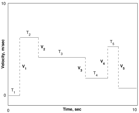
Figure 1: Single realization of a continuous time random walk with random waiting-times $T_{i}$ between successive random jumps of velocity $V_{i}$.

Although the random process $S(t)$ is self-similar, it has neither stationary nor independent increments, and all its moments are finite Bingham (1971); H$\ddot{\rm o}$pfner (1990). This process is non-Markovian, but it is inverse to the continuous limit of a Markov random process of temporal steps $T(\tau)$, i. e. $S(T(\tau))=\tau$. The analytical form of the probability density of the random variable $S(t)$ can be calculated as follows. According to Bingham (1971), the expectation $\langle e^{-vS(t)}\rangle=\int^{\infty}_{0}dx\,e^{-vx}\,p^{S}(t,x)$ is equal to the Mittag-Leffler function $E_{\alpha}(-vt^{\alpha})$. After the Laplace transform of the Mittag-Leffler function with respect to $t$, the expectation can be easily inverted analytically with respect $v$. Then the probability density of the process $S(t)$ is written as

$$p^{S}(t,\tau)=\frac{1}{2\pi i}\int_{Br}e^{ut-\tau u^{\alpha}}\,u^{\alpha-1}\,du\,,$$ (2)

where $Br$ denotes the Bromwich path. This probability density characterizes the probability to be at the internal time $\tau$ on the real time $t$. After the variable transform $ut\to u$ and denoting $z=\tau/t^{\alpha}$, the function $p^{S}(t,\tau)$ takes the form $t^{-\alpha}F_{\alpha}(z)$, where $F_{\alpha}(z)=\frac{1}{2\pi i}\int_{Br}e^{u-zu^{\alpha}}\,u^{\alpha-1}\,du$. On deforming the Bromwich path into the Hankel path, we find the Taylor series of the function $F_{\alpha}(z)$, i. e.

$$F_{\alpha}(z)=\sum_{k=0}^{\infty}\frac{(-z)^{k}}{k!\Gamma(1-\alpha-k\alpha)}\,,$$ (3)

where $\Gamma(x)$ is the usual Gamma function. Since the radius of convergence of the power series (3) can be proven to be infinite for $0<\alpha<1$, the function $F_{\alpha}(z)$ is entire in $z$. Thus, the exchange between the series and the integral in the calculations of the Taylor series (3) is quite legitimate. The Laplace image of the function $F_{\alpha}(z)$ is expressed in terms of the Mittag-Leffler function

$$\int^{\infty}_{0}e^{-z\zeta}\,F_{\alpha}(z)\,dz=E_{\alpha}(-\zeta)\,,\quad z>0.$$

Feller conjectured and Pollard proved in 1948 that the Mittag-Leffler function $E_{\alpha}(-x)=\sum_{n=0}^{\infty}(-x)^{n}/\Gamma(1+n\alpha)$ is completely monotonic for $x\geq 0$, if $0<\alpha\leq 1$. Moreover, $E_{\alpha}(-x)$ is an entire function of order $1/\alpha$ for $\alpha>0$ Feller (1971). Hence, by Feller Feller (1971), one can conclude that the function $F_{\alpha}(z)$ is non-negative in $z>0$. Taking into account the normalization relation $\int_{0}^{\infty}F_{\alpha}(z)\,dz=1$, the function $p^{S}(t,\tau)$ is just a probability density. If $\alpha=1/2$, from the series (3) it is easy to recognize the well-known Gaussian function $F_{\alpha}(z)=\pi^{-1/2}\exp(-z^{2}/4)$. It should be observed here that the basic Cauchy and Signaling problems of the time fractional diffusion-wave equation can be expressed in terms of the function $F_{\alpha}(z)$ (see more details in Mainardi (1996)).

III Fractional Fokker-Planck equation

The Langevin equation directed by the stochastic time clock $S(t)$ can be written in the form

$$d{\bm{V}}(S(t))=-\gamma{\bm{V}}(S(t))\,dS(t)+d{\bm{W}}(S(t)).$$ (4)

The statement is quite justified. The process ${\bm{V}}(S(t))$ is a continuous martingale, and the directing process $S(t)$ is a continuous submartingale with respect to an appropriate filtration H$\ddot{\rm o}$pfner (1990). All the moments of both parent and directing processes are finite. The same concerns the process ${\bm{V}}(S(t))$. Now the random walk of a particle is defined by two Markov processes, random waiting times $T(\tau)$ between random jumps ${\bm{V}}(\tau)$. The discrete example of such a walk is shown in Fig. 1. A similar approach, i. e. the modeling of anomalous diffusion by two independent random processes indexed by a common continuous parameter, has been already suggested in 16 . However, the inverse process to the time evolution was not completely defined. It was not recognized as a first passage process. No direct relationship between Eqs. (1) and (4) was found. This is also a main difference between the subject of Sokolov (2001) and our paper.

The resulting process ${\bm{V}}(S(t))$ is subordinated to ${\bm{V}}(t)$, called the parent process, and is directed by $S(t)$, called the directing process Feller (1971). The hitting time process $S(t)$ just satisfies necessary properties imposed on any directing process (independent, positive and non-decreasing). The directing process is often referred to as the randomized time or operational time. In other words, the subordinated process ${\bm{V}}(S(t))$ is obtained by randomizing the time clock of a random process ${\bm{V}}(t)$ using a random process $S(t)$. In compliance with Feller (1971), the probability density of the random process ${\bm{v}}_{t}={\bm{V}}(S(t))$ is expressed by the integral relation

$$p^{\,v_{t}}({\bm{V}},t)=\int^{\infty}_{0}p^{V}({\bm{V}},\tau)\,p^{S}(t,\tau)\,d\tau\,,$$ (5)

where $p^{V}({\bm{V}},\tau)$ represents the probability to find the random value ${\bm{V}}$ on the internal time $\tau$. Recall that $p^{S}(t,\tau)$ is the probability to be at the operational time $\tau$ on the real time $t$. It is well known that the stochastic differential equation of type (1) is equivalent to the corresponding FPE. In particular, the probability density $p^{V}({\bm{V}},\tau)$ obeys the standard FPE

$$\frac{\partial p^{V}({\bm{V}},\tau)}{\partial\tau}={\hat{L}}_{\rm FP}\,p^{V}({\bm{V}},\tau),$$

where ${\hat{L}}_{\rm FP}$ is a time-independent Fokker-Planck operator whose exact form is not important here. The Laplace transform of the function $p^{\,v_{t}}({\bm{V}},t)$ with respect to time replaces the integral relation (5) by the algebraic one, $\bar{p}^{\,v_{t}}({\bm{V}},u)=u^{\alpha-1}\bar{p}^{V}({\bm{V}},u^{\alpha})$. Acting the operator ${\hat{L}}_{\rm FP}$ on the Laplace image, we obtain $[{\hat{L}}_{\rm FP}\,\bar{p}^{\,v_{t}}]({\bm{V}},u)=u^{\alpha}\,\bar{p}^{\,v_{t}}({\bm{V}},u)-Q({\bm{V}})\,u^{\alpha-1}$, where $Q({\bm{V}})$ is the initial condition. The inverse Laplace transform gives the fractional FPE

$$p^{\,v_{t}}({\bm{V}},t)= Q({\bm{V}})+$$

$$+\,\,\,\frac{1}{\Gamma(\alpha)} \!\!\!\int_{0}^{t}d\tau\,(t-\tau)^{\alpha-1}\,[{\hat{L}}_{\rm FP}\,p^{\,v_{t}}]({\bm{V}},\tau).$$ (6)

This equation has also the equivalent form

$$\frac{\partial^{\alpha}p^{\,v_{t}}({\bm{V}},t)}{\partial t^{\alpha}}-\frac{Q({\bm{V}})\,t^{-\alpha}}{\Gamma(1-\alpha)}={\hat{L}}_{\rm FP}\,p^{\,v_{t}}({\bm{V}},t)\,,$$

where $\partial^{\alpha}/\partial t^{\alpha}$ denotes the Liouville-Riemann fractional differential operator of order $\alpha$ Samko (1993). Our analysis generalizes the mathematical treatment of Sokolov (2001) and shows that the Fokker-Planck operator can have a more general form rather than only with a temporally constant force field. Another approach to the description of anomalous transport in external fields is developed in 20 . The consideration is based on a generalization of the classical Chapman-Kolmogorov equation. An interesting justification of the generalized Chapman-Kolmogorov equation is that trapping events are superimposed on the Langevin dynamics, with a waiting time distribution with infinite mean. By the choice of special forms for the transfer kernel and the probability density function of the waiting time between any two successive jump events in the generalized equation, one can recover some models discussed in the literature.

If the probability density $p^{V}({\bm{V}},\tau)$ is known explicitly, the solution of (6) can be calculated by mean of

$$p^{\,v_{t}}({\bm{V}},t)=\int^{\infty}_{0}F_{\alpha}(z)\,p^{V}({\bm{V}},t^{\alpha}z)\,dz\,.$$ (7)

The formula is especially useful for some particular cases whose the exact solutions of the ordinary FPE have a closed form (for example, the harmonic potential leading to a linear force field in FPE). It is interesting also to observe the integral representation of the fractional FPE solution in Barkai and Silbey (2000) (see expression (2.32)). Now clearly, that formula is nothing else as a consequence of the subordination relation (5) (or (7)). In this connection it should be noted that the relation (5) is not of convolution type, so the derivation of Eq. (6), having the fractional integral of time, from the ordinary FPE is not entirely trivial.

Many papers E. Barkai (2000); Stanislavsky (2000); R. Metzler (1998); Saichev and Zaslavsky (1997); R. Metzler (1999); Rangarajan and Ding (2000); Barkai and Silbey (2000) have focused on the derivation of the fractional FPE with different potentials and its solution. Starting with Montroll and Weiss (1965), the continuous time random walk approach is very popular for that goal. However, only recently it has been shown that the solutions are density functions of a stochastic process Meerschaert and Scheffler (2001). We support the latter point of view: the problem of anomalous diffusion should be analyzed with the exact definition of the corresponding random process. The density function and the master equation are derived from this process.

IV Fluctuation-dissipation relation and H-theorem

According to Eq. (1), the variance of the random variable $\bm{V}$ is

$$\langle V^{2}_{i}(\tau)\rangle=v^{2}_{i,\,0}\,e^{-2\gamma\tau}+\frac{D}{\gamma}\left(1-e^{-2\gamma\tau}\right),$$ (8)

where $v_{i,0}$ is the initial condition. Since the random processes $\bm{V}$ and $S(t)$ are independent, we average the expression (8) on the internal variable $\tau$ so that

$$\overline{\langle V^{2}_{i}(t)\rangle}=\int^{\infty}_{0}F_{\alpha}(z)\,\langle V^{2}_{i}(t^{\alpha}z)\rangle\,dz\,,$$ (9)

where the line over a variable denotes the average over the internal variable $\tau$. Calculating the following integral

$$\int_{0}^{\infty}F_{\alpha}(z)\,e^{-2\gamma t^{\alpha}z}\,dz=E_{\alpha}(-2\gamma t^{\alpha})\,,$$ (10)

the exponential functions in (8) are replaced with the Mittag-Leffler function for (9). The stationary state of (4) is finite so that

$$\lim_{t\to\infty}\overline{\langle V^{2}_{i}(t)\rangle}=D/\gamma\,.$$ (11)

The constants $D$ and $\gamma$ are interpreted as generalized diffusion and damping coefficients respectively. The mean $\overline{\langle V_{i}(t)\rangle}$ is zero as well as $\langle V_{i}(\tau)\rangle=0$. The boundary case $\alpha=1$ may be also included in the study, as $S(t)=t$. The probability density $p^{S}(t,\tau)$ reduces to the Dirac $\delta$-function, and Eq. (1) becomes the ordinary Langevin equation in the true time $t$.

In the other hand, the energy of a classical system is distributed equally among all degrees of freedom. We get the fluctuation-dissipation relation $D/\gamma=k_{B}T/m$ for the given temperature of a bath $T$ and the mass of a particle $m$, and $k_{B}$ is the Boltzmann constant. The expression is very similar to the Einstein relation, but the constants $D$ and $\gamma$ are generalized. It should be pointed out that the stochastic time arrow does not break this equal distribution law and influences only on the character of relaxation (slow power decay). Therefore, in this case the concept of temperature is valid, i. e. the stationary state of the fractional FPE is defined by the temperature $T$. The difference of entropies of equilibrium and arbitrary states gives a Lyapunov functional $\Lambda(t)\geq 0$. No wonder that its temporal evolution confirms the H-theorem. Although the law of relaxation toward thermal equilibrium changes, it remains monotonic, and the equilibrium state has the most entropy due to the Gibbs-Boltzmann distribution. The fact, that no modifications of the Boltzmann thermodynamics for anomalous diffusion described by the equation of type (6) are required, was already noted in R. Metzler (1999); Barkai and Silbey (2000); I.M. Sokolov (2001). However, the true cause of the result was not established. Now it is clear that both processes (1) and (4) are closely connected and have a common ground.

V General kinetic equation with the stochastic time clock

For a general type of a Markovian process the general kinetic equation is

$$\frac{dp_{n}(t)}{dt}=\sum_{k=0}^{\infty}\left\{W_{nk}p_{k}(t)-W_{kn}p_{n}(t)\right\}\,,$$ (12)

where $W_{kn}$ are the transition probability rates from state $n$ to state $k$. This equation defines the probability $p_{n}$ for the system to be in state $n$. The term $W_{nk}p_{k}$ describes transitions into the state $n$ from states $k$, and $W_{kn}p_{n}$ corresponds to transition out of $n$ into other states $k$. The continuous version of Eq. (12) takes the form

$$\frac{dP(y,t)}{dt}=\int\left\{W(y\mid y^{\prime})P(y^{\prime},t)-W(y^{\prime}\mid y)P(y,t)\right\}dy^{\prime}\,$$

with the initial condition $P(y,0)$. Let us represent both these equations as

$$\frac{dp\,(t)}{dt}=\hat{\bm{W}}p\,(t)\,,$$ (13)

where $\hat{\bm{W}}$ denotes the transition rate operator. It is important to emphasize here that this operator is time-independent. The equation (13) can be written in the integral form

$$p\,(t)=p\,(0)+\int^{t}_{0}d\tau\,\hat{\bm{W}}p\,(\tau)\,.$$

The Laplace transform $\tilde{p}\,(s)$ with respect to $t$ is given by

$$\tilde{p}\,(s)=\int_{0}^{\infty}e^{-st}\,p\,(t)\,dt$$

and leads to

$$\hat{\bm{W}}\,\tilde{p}\,(s)=s\tilde{p}\,(s)-p\,(0)\,.$$

Now we determine a new process with the probability equal to

$$p_{\alpha}(t)=\int_{0}^{\infty}p^{S}(t,\tau)\,p\,(\tau)\,d\tau\,.$$

In Laplace space the probabilities $p_{\alpha}(t)$ and $p\,(t)$ are related by $\tilde{p}_{\alpha}(s)=s^{\alpha-1}\tilde{p}\,(s^{\alpha})$, where

$$\tilde{p}_{\alpha}(s)=\int_{0}^{\infty}e^{-st}\,p_{\alpha}(t)\,dt$$

is the Laplace image of $p_{\alpha}(t)$. By the simple algebraic transformations we find

$$\hat{\bm{W}}\,\tilde{p}_{\alpha}(s) = s^{\alpha-1}\,\hat{\bm{W}}\,\tilde{p}\,(s^{\alpha})$$ (14)

$$= s^{\alpha-1}\,\{s^{\alpha}\,\tilde{p}\,(s^{\alpha})-p\,(0)\}$$

$$= s^{\alpha}\tilde{p}_{\alpha}(s)-p\,(0)\,s^{\alpha-1}\,.$$

Thus, the fractional extension of Eq. (13) reads

$$p_{\alpha}(t)=p\,(0)+\frac{1}{\Gamma(\alpha)}\int^{t}_{0}d\tau\,(t-\tau)^{\alpha-1}\hat{\bm{W}}\,p_{\alpha}(\tau)\,.$$ (15)

For $\alpha=1$ we recover Eq. (13). For a system with discrete states the generating function is of the form

$$G(\zeta,t)=\sum_{k=0}^{\infty}\zeta^{k}p_{k}(t)\,,$$

where the restriction $\mid\zeta\mid\leq 1$ is imposed to ensure convergence of the series. With the help of the generating function, one can find the moments by taking the derivative with respect to $\zeta$ and then setting $\zeta=1$. The generating function of the process governed by the stochastic time clock is given by the relation

$$G_{\alpha}(\zeta,t)=\int^{\infty}_{0}F_{\alpha}(z)\,G(\zeta,t^{\alpha}z)\,dz\,.$$ (16)

Thus, the generating function for a discrete Markov process directed by the process $S(t)$ can be obtained from the appropriate generating function of the parent process by immediate integration.

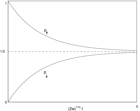
Figure 2: The relaxation of the probabilities $p_{\uparrow}$ [Eq.(17)] and $p_{\downarrow}$ [Eq.(18)] plotted as a function of time. The dotted line corresponds to the equilibrium state.

As an example, we consider the relaxation in a two-state system. Let $N$ be the common number of objects in this system. If $N_{\uparrow}$ is the number of objects in the state $\uparrow$, $N_{\downarrow}$ is the number of objects in the state $\downarrow$ so that $N=N_{\uparrow}+N_{\downarrow}$. Assume that for $t=0$ the states $\uparrow$ dominate, i. e.

$$\frac{N_{\uparrow}(t=0)}{N}=p_{\uparrow}(0)=1,\quad\frac{N_{\downarrow}(t=0)}{N}=p_{\downarrow}(0)=0\,,$$

where $p_{\uparrow}$ and $p_{\downarrow}$ are the probabilities to find the system in the states $\uparrow$ and $\downarrow$ respectively. Denote the transition rates by $w$. In the case the general kinetic equation with the stochastic time clock (15) is written as

$$p_{\uparrow}(t) = p_{\uparrow}(0)+\frac{w}{\Gamma(\alpha)}\int^{t}_{0}(t-\tau)^{\alpha-1}\,\{p_{\downarrow}(\tau)-p_{\uparrow}(\tau)\}d\tau,$$

$$p_{\downarrow}(t) = p_{\downarrow}(0)+\frac{w}{\Gamma(\alpha)}\int^{t}_{0}(t-\tau)^{\alpha-1}\,\{p_{\uparrow}(\tau)-p_{\downarrow}(\tau)\}d\tau.$$

From the linearity of these equations it follows

$$p_{\uparrow}(t)+p_{\downarrow}(t) = p_{\uparrow}(0)+p_{\downarrow}(0)\,,\quad p_{\uparrow}(t)-p_{\downarrow}(t)=$$

$$p_{\uparrow}(0)-p_{\downarrow}(0) - \frac{2w}{\Gamma(\alpha)}\int^{t}_{0}(t-\tau)^{\alpha-1}\,\{p_{\uparrow}(\tau)-p_{\downarrow}(\tau)\}d\tau.$$

Consequently, we obtain

$$p_{\uparrow}(t)=\frac{1}{2}+\frac{1}{2}E_{\alpha}(-2wt^{\alpha}),$$ (17)

$$p_{\downarrow}(t)=\frac{1}{2}-\frac{1}{2}E_{\alpha}(-2wt^{\alpha}).$$ (18)

The steady state of the system corresponds to equilibrium, $p_{\uparrow}(\infty)=p_{\downarrow}(\infty)=1/2$ (Fig. 2). The transition rate $w$ is defined by microscopic properties of the system (for instance, from the given Hamiltonian of interaction and the Fermi’s golden rule). The value $(2w)^{-1/\alpha}$ may be interpreted as a generalized relaxation time. The randomization of time clock essentially changes the character of relaxation in such a two-state system. If only $\alpha\neq 1$, the relaxation has an algebraic decay. In this connection it should be mentioned here that the experimental relaxation curves of glasses show just the algebraic decay Gl$\ddot{\rm o}$ckle and Nonnenmacher (1991).

VI Summary

We have shown that the fractional FPE can be derived by using the ordinary Langevin equation. Although the processes described by Eq. (6) are non-Markovian at the true time, they are Markovian with regard to the internal time. So the strange kinetics results in the randomization of time clock of a Markov process. In the probability theory the operation is called the subordination of one random process by another Feller (1971). As has been stated above, the subordination does not break the fluctuation-dissipation relation and the H-theorem. The stochastic time clock has a clear physical sense – a particle interacts with a bath in random points of time so that there are memory effects. It should be noted that the memory is a direct consequence of the random time steps belonging to the strict domain of attraction of a $\alpha$-stable distribution. One and only one index $\alpha$ characterizes both the corresponding $\alpha$-stable process and its hitting time process. The stochastic differential equation (4) describes a random velocity field directed by a random Markov process. In this case the dynamical foundation of statistical physics is valid. The procedure of the randomization of time clock extends the domain of applicability for the general kinetic equation.