QUANTUM FIELD THEORY IN GRAPHENE

Abstract

This is a short non-technical introduction to applications of the Quantum Field Theory methods to graphene. We derive the Dirac model from the tight binding model and describe calculations of the polarization operator (conductivity). Later on, we use this quantity to describe the Quantum Hall Effect, light absorption by graphene, the Faraday effect, and the Casimir interaction.

PACS numbers: 73.63.-b, 11.10.Kk

1 Introduction

Graphene, which is a one-atom thick layer of carbon atoms has many exceptional properties[1, 2, 3] making it one of the most interesting topics in condensed matter physics. The principle feature of graphene is that the quasi-particle excitations satisfy the Dirac equation, where the speed of light $c$ is replaced by the so-called Fermi velocity $v_{F}\simeq c/300$. Therefore, the quantum field theory methods are very useful in the physics of graphene. By applying these methods, one can explain anomalous Hall Effect in graphene, the universal optical absorption rate, the Faraday effect, and predict the Casimir interaction of graphene, and do much more.

The purpose of this article is to give a non-technical introduction to and a short overview of the use of quantum field theory in graphene. We start in the next Section with a derivation of the Dirac model from the tight binding model and a discussion of possible generalizations of the former. Quantum filed theory calculations in the Dirac model are presented in Sec. 3 at the example of polarization operator. This operator is then used in Sec. 4.1 to explain the anomalous Hall conductivity of graphene, which is proportional to $n+1/2$ with an integer $n$. Next, in Sec. 4.2 we derive the universal absorption rate of $\alpha\pi\simeq 2.3\%$ for optical frequencies. Sec. 4.3 is devoted to explanations of the measured giant Faraday effect in graphene and to further study of the polarization rotation. Sec. 4.4 contains a survey of calculations of the Casimir interaction of graphene.

2 The Dirac model

The Dirac model for quasi-particles in graphene was elaborated in full around 1984[4, 5] – twenty years before actual discovery of graphene. However, its basic properties, like the linearity of the spectrum, etc., were well known and widely used much earlier due to the 1947 paper by Wallace[6]. The purpose of most of the works of the time was to describe graphite rather than graphene. For more details on the development and formulation of the Dirac model we refer the reader to a recent review[7].

In graphene, the carbon atoms form a honeycomb lattice (see Fig. 1) with two triangular sublattices A and B. The lattice spacing is $d=1.42$Å. The nearest neighbors of an atom from the sublattice A belong to the sublattice B, and vice versa. By adding to the location of an atom in the sublattice A any of the three vectors

$${\bf\delta}_{1}=d(-1,0),\qquad{\bf\delta}_{2}=d(1/2,\sqrt{3}/2),\qquad{\bf\delta}_{3}=d(1/2,-\sqrt{3}/2)$$ (1)

one arrives to the location of one of the nearest neighbors in the sublattice B.

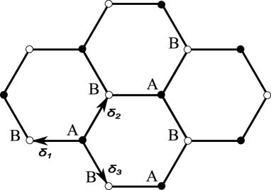
Figure 1: The honeycomb lattice of graphene.

In the tight binding model only the interaction between electrons belonging to the nearest neighbors is taken into account, so that the Hamiltonian reads

$$H=-t\sum_{\alpha\in A}\sum_{j=1}^{3}\Bigl{(}a^{\dagger}({\bf r}_{\alpha})b({\bf r}_{\alpha}+{\bf\delta}_{j})+b^{\dagger}({\bf r}_{\alpha}+{\bf\delta}_{j})a({\bf r}_{\alpha})\Bigr{)}\,,$$ (2)

where $t$ is the so-called hopping parameter, and the operators $a^{\dagger}$, $a$, $b^{\dagger}$, $b$ are creation and annihilation operators of electrons in the sublattices A and B, respectively. We adopt the units $\hbar=c=1$. These operators satisfy usual anticommutation relations. Let us represent the wave function through a Fourier transform.

$$|\psi\rangle=\Bigl{(}\psi_{A}({\bf k})\sum_{\alpha\in A}e^{i{\bf k}{\bf r}_{\alpha}}a^{\dagger}({\bf r}_{\alpha})+\psi_{B}({\bf k})\sum_{\beta\in B}e^{i{\bf k}{\bf r}_{\beta}}b^{\dagger}({\bf r}_{\beta})\Bigr{)}|0\rangle$$ (3)

The sublattice A is generated by shifts along the vectors ${\bf\delta}_{2}-{\bf\delta}_{1}$ and ${\bf\delta}_{3}-{\bf\delta}_{1}$. Therefore, two momenta ${\bf k}_{1}$ and ${\bf k}_{2}$ are equivalent if $(n_{1}({\bf\delta}_{2}-{\bf\delta}_{1})+n_{2}({\bf\delta}_{3}-{\bf\delta}_{1}))\cdot({\bf k}_{1}-{\bf k}_{2})\in 2\pi\mathbb{Z}$ for all integer $n_{1}$ and $n_{2}$. Representatives of the equivalence classes can be taken in a compact region in the momentum space – the Brillouin zone, which is a hexagon with the corners at the points $v_{1}=2\pi/3d\left(1,1/\sqrt{3}\right)$, $v_{2}=2\pi/3d\left(1,-1/\sqrt{3}\right)$, $v_{3}=2\pi/3d\left(0,-2/\sqrt{3}\right)$, $v_{4}=-v_{1}$, $v_{5}=-v_{2}$ and $v_{6}=-v_{3}$. Opposite sides of this hexagon are identified, and, in particular, the corners $v_{1}$, $v_{3}$ and $v_{5}$ are equivalent between themselves, as well as $v_{2}$, $v_{4}$ and $v_{6}$ are.

One can calculate

$$H|\psi\rangle=-t\Bigl{(}\psi_{B}\sum_{j=1}^{3}e^{i{\bf k}{\bf\delta}_{j}}\sum_{\alpha\in A}e^{i{\bf k}{\bf r}_{\alpha}}a^{\dagger}({\bf r}_{\alpha})+\psi_{A}\sum_{j=1}^{3}e^{-i{\bf k}{\bf\delta}_{j}}\sum_{\beta\in B}e^{i{\bf k}{\bf r}_{\beta}}b^{\dagger}({\bf r}_{\beta})\Bigr{)}|0\rangle$$ (4)

so that the stationary Schrödinger equation $H|\psi\rangle=E|\psi\rangle$ becomes the matrix equation

$$\left(\begin{array}[]{cc}0&-tX\\ -tX^{*}&0\end{array}\right)\left(\begin{array}[]{c}\psi_{A}\\ \psi_{B}\end{array}\right)=E\left(\begin{array}[]{c}\psi_{A}\\ \psi_{B}\end{array}\right)\,,\qquad X=\sum_{j=1}^{3}e^{i{\bf k}{\bf\delta}_{j}}\,.$$ (5)

Clearly, the eigenvalues read

$$E=\pm t|X|\,.$$ (6)

The spectrum is symmetric, with positive and negative parts meeting at the points where $X=0$. Solutions to this condition are easy to find, and they coincide with the corners of the Brillouin zone. As we have discussed above, only two of the corners are independent. Let us take $K_{\pm}=\pm v_{6}=\mp v_{3}$ as two independent solutions, called the Dirac points, describing two independent ground states.

The next step is to expand the wave functions around these Dirac points, $\psi^{\pm}_{A,B}({\bf q})\equiv\psi_{A,B}(K_{\pm}+{\bf q})$. We suppose here that $|{\bf q}|$ is small compared to $1/d\sim 1{\rm KeV}$. Then, one obtains the Hamiltonians

$$H_{\pm}=\frac{3td}{2}\left(\begin{array}[]{cc}0&iq_{1}\pm q_{2}\\ -iq_{1}\pm q_{2}&0\end{array}\right)=v_{F}(-\sigma_{2}q_{1}\pm\sigma_{1}q_{2})\,,$$ (7)

where $v_{F}$ is the Fermi velocity, $\sigma_{i}$ are the standard Pauli matrices. By substituting in $v_{F}=(3td)/2$ the value of $d$ given above and $t=2.8{\rm eV}$ one obtains a number which is slightly below the commonly accepted value $v_{F}\simeq 1/(300)$. By introducing a four-component spinor $\psi\equiv(\psi_{A}^{+},\psi_{B}^{+},\psi_{A}^{-},\psi_{A}^{-})$, we can unify $H_{\pm}$ in a single Dirac Hamiltonian $H=-iv_{F}\gamma^{0}\gamma^{a}\partial_{a}$, $a=1,2$, where we replaced the momenta $i{\bf q}$ by partial derivatives, and

$$\gamma^{0}=\left(\begin{array}[]{cc}\sigma_{3}&0\\ 0&\sigma_{3}\end{array}\right),\qquad\gamma^{1}=\left(\begin{array}[]{cc}i\sigma_{1}&0\\ 0&i\sigma_{1}\end{array}\right),\qquad\gamma^{2}=\left(\begin{array}[]{cc}i\sigma_{2}&0\\ 0&-i\sigma_{2}\end{array}\right).$$ (8)

These $4\times 4$ gamma matrices are taken in a reducible representation which is a direct sum of two inequivalent $2\times 2$ representations.

Each of these two-component representations for graphene quasiparticles’ wave-function is somewhat similar to the spinor description of electrons in QED₃₊₁. However, in the case of graphene this pseudo spin index refers to the sublattice degree of freedom rather than the real spin of the electrons. The whole effect of the real spin, which by now did not appear in presented Dirac model, is just in doubling the number of spinor components, so that we have 8-component spinors in graphene ($N=4$ species of two–component fermions).

We conclude, that the tight binding model is equivalent below the energies $1/d$ to a quasi-relativistic Dirac model, where the speed of light is replaced by $v_{F}$. One should keep in mind that the tight binding model itself is an approximation. One can improve this approximation by considering, for example, couplings between atoms in the same lattice A or B, that is a next-nearest neighbor coupling. The corresponding energy is estimated to be about $0.1\,{\rm eV}$, much smaller than the nearest neighbor coupling $t$ considered above. Other possible couplings are summarized in Ref. Gusynin:2007ix. It is expected that with suitable modifications the Dirac model is valid at least until the energies of $\sim 2\,{\rm eV}$.

Under various circumstances, it may make sense to consider the following modifications of the Dirac model.

• One can add an interaction with the electromagnetic field. To preserve gauge invariance, this interaction is introduced by replacing the usual partial derivatives by gauge-covariant ones: $\partial\to\partial+ieA$. The electromagnetic potential is not confined to the graphene surface, but rather propagates in the ambient $3+1$ dimensional space. This field may be an external magnetic field, a classical electromagnetic radiation, or quantized fluctuations.

• Quasiparticles may have a mass. This mass is usually very small, but the introduction of a mass parameter may be convenient on theoretical grounds, e.g., to perform the Pauli-Villars regularization.

• A more important mass-like parameter is the chemical potential $\mu$, which describes the quasiparticle density. This parameter can be easily varied in experiments by applying a gate potential to graphene samples. Without a gate potential, $\mu$ is usually very small in a suspended graphene, but can be significant for epitaxial graphene due to interaction with the substrate.

• Impurities in graphene are described by adding a phenomenological parameter $\Gamma$ which reminds an imaginary mass and enters the propagator of quasiparticles exactly as $\epsilon$ in the Feynman prescription of contour integration.

• Finally, most experiments with graphene are done at rather high temperatures, which can be taken into account by usual rules of real or imaginary time thermal field theory.

3 Polarization operator

Let us proceed with quantum field theory calculations based on the Dirac model. From the Dirac Hamiltonian one can derive the action

$$S=\int d^{3}x\bar{\psi}\not{D}\psi\,,\qquad\not{D}=i\tilde{\gamma}^{j}(\partial_{j}+ieA_{j})+\dots$$ (9)

where the dots denote any of additional terms described at the end of the previous section. Tilde over $\gamma$ means that the space-components are rescaled

$$\tilde{\gamma}^{0}=\gamma^{0},\qquad\tilde{\gamma}^{1,2}=v_{F}\gamma^{1,2}\,.$$ (10)

Quantized fermions give rise to an effective action for external electromagnetic field (given by a sum of one-loop diagrams). To the second order in $A$, it reads

$$S_{\rm eff}(A)=A\ \raisebox{-10.66977pt}{\psfig{height=28.90755pt}}\ A=\frac{1}{2}\int\frac{d^{3}p}{(2\pi)^{3}}A_{j}(-p)\Pi^{jl}(p)A_{l}(p),$$ (11)

where $\Pi^{jl}$ is the polarization operator.

As an example, let us consider the polarization operator for a single massive two-component fermion at zero temperature, zero chemical potential, and without external magnetic field. Simple calculations give

$$\Pi^{mn}=\frac{\alpha}{v_{F}^{2}}\,\eta^{m}_{j}\left[\Psi(p)\left(g^{jl}-\frac{\tilde{p}^{j}\tilde{p}^{l}}{\tilde{p}^{2}}\right)+i\phi(p)\epsilon^{jkl}\tilde{p}_{k}\right]\eta_{l}^{n}$$ (12)

with $\epsilon^{jkl}$ being the Levi-Civita totally antisymmetric tensor normalized according to $\epsilon^{012}=1$, $\eta_{j}^{n}={\rm diag}(1,v_{F},v_{F})$, $\tilde{p}^{m}\equiv\eta_{n}^{m}p^{n}$. $\alpha=e^{2}/(4\pi)\simeq 1/137$ is the fine structure constant. The tensor structure of $\Pi^{mn}$ is uniquely defined by quasi-relativistic and gauge invariances up to two functions, $\Psi$ and $\phi$, which read

$$\Psi(p)=\frac{2m\tilde{p}-(\tilde{p}^{2}+4m^{2}){\rm arctanh}({\tilde{p}}/{2m})}{2\tilde{p}},$$ (13)

$$\phi(p)=\frac{2m\,{\rm arctanh}(\tilde{p}/2m)}{\tilde{p}}-1$$ (14)

here $\tilde{p}\equiv+\sqrt{\tilde{p}_{j}\tilde{p}^{j}}$, and we assume $m>0$. From Eq. (12) one might get an impression that the polarization tensor is singular at the $v_{F}\to 0$ limit, or, that $\Pi^{jk}$ is greatly enhanced by the smallness of $v_{F}$. A more careful analysis shows that it is not true, the polarization tensor remains finite in the $v_{F}\to 0$ limit provided the frequency is non-vanishing, $p_{0}\neq 0$.

For more complicated external conditions, like a magnetic field, or for a non-zero chemical potential, the quasi-Lorentz invariance is broken, and the polarization tensor has a more complicated form than Eq. (12).

Particular importance of $\Pi^{jk}$ is due to the fact that this tensor defines how the electromagnetic field propagates through graphene. The full quadratic action for electromagnetic field is $-\frac{1}{4}\int d^{4}x\,F^{2}_{\mu\nu}+S_{\rm eff}$, where the effective action (11) is confined to the surface of graphene, which we place at $x^{3}=0$. The equations of motion following from this action contain a singular term

$$\partial_{\mu}F^{\mu\nu}+\delta(x^{3})\Pi^{\nu\rho}A_{\rho}=0.$$ (15)

We extended $\Pi$ to a $4\times 4$ matrix with $\Pi^{3\mu}=\Pi^{\mu 3}=0$. The equations (15) describe a free propagation of the electromagnetic field outside the surface $x^{3}=0$ subject to the matching conditions

$$A_{\mu}|_{x^{3}=+0}=A_{\mu}|_{x^{3}=-0},$$

$$(\partial_{3}A_{\mu})|_{x^{3}=+0}-(\partial_{3}A_{\mu})|_{x^{3}=-0}=\Pi_{\mu}^{\ \nu}A_{\nu}|_{x^{3}=0}$$ (16)

on that surface.

The polarization tensor and, more generally, Feynman diagrams involving $2+1$ dimensional fermions were considered in a large number of papers. Still in 1980’s the function $\Psi$ (for $v_{F}=1$) was calculated in Ref. Appelquist, while the pseudotensor part was discussed about the same time in the context of the parity anomaly[10, 11]. A renormalization group approach to theories with $v_{F}\neq 1$ was suggested in Ref. Voz1. In this century, extensive calculations were done by the Kiev group and collaborators[13, 14, 15, 16]. The formulas (12), (13) and (14) are consistent with that calculations.

4 Physical effects

We proceed with considering some quantum field theory effects in graphene. Specifically, we will be interested in applications of the polarization tensor $\Pi^{ij}$. We shall see, that this quantity indeed defines important and interesting physics.

4.1 Quantum Hall Effect

First of all, we note that the polarization tensor can be interpreted in terms of the conductivity of graphene. Indeed, variation of the effective action (11) with respect to $A_{k}$ produces an expectation value of the electric current in graphene, i.e. $j^{k}\simeq\Pi^{kl}A_{l}$. On the other hand, in the temporal gauge, $A_{0}=0$, the electric field $E_{a}$ with the frequency $\omega$ is related to the vector potential by $E_{a}=i\omega A_{a}$. By definition, the conductivity is a matrix relating $j$ and $E$. In this way, one arrives at the relation

$$\sigma_{ab}=\frac{\Pi_{ab}}{i\omega}\,,\quad a,b=1,2.$$ (17)

To study the conductivity tensor at zero frequency (the dc conductivity) one puts the graphene sample in a constant magnetic field perpendicular to its surface and measures the anti-diagonal conductivity as a function of the chemical potential $\mu$. This is precisely the set-up for Hall experiments. For a one-layer graphene it was observed[17, 18] that the off-diagonal (Hall) conductivity is quantized according to the law

$$\sigma_{12}\sim\Bigl{(}n+\frac{1}{2}\Bigr{)},\qquad n=0,1,2,\dots$$ (18)

i.e., the conductivity is proportional to half-integer numbers. This particular type of the Hall Effect is called anomalous, or unconventional integer, or half-integer Quantum Hall Effect. Starting with the Dirac model, the behavior (18) was predicted in Ref. TQHE1 by using the Feynman diagram approach described above, and in Ref. TQHE2 from numerical simulations. This wonderful agreement between theory and experiment was the first confirmation of existence of the Dirac quasi-particles in graphene.

It is interesting to note, that the half-integer Quantum Hall Effect is observed in the mono-layer graphene only. The double-layer graphene, for example, exhibits conventional Integer Quantum Hall Effect. This does not however imply that the Dirac model is not applicable to double-layer graphenes. The later case may be recovered if one carefully considers phases of determinant of the Dirac operator[21, 22].

4.2 Absorption of light

Another physical effect defined by the polarization operator is the absorption of light by a suspended monolayer graphene. In the simplest set-up one can neglect the chemical potential, suppose that there is no external magnetic field and put temperature to zero, $T=0$. Consequently, one can use the polarization operator (12), where, because of $N=4$ generations of fermions in graphene, the scalar part $\Psi$ is multiplied by $N$, while the pseudo-scalar part $\phi$ cancells out. The cancellation occurs due to the form of gamma-matices (8), containing two inequivalent representations related by the parity transformations. In other words, we need to make a substitution

$$\Psi\to\Psi_{N}=N\Psi,\qquad\phi\to 0\,.$$ (19)

Let us consider a plane wave with the frequency $\omega$ propagating along the $x^{3}$-axis from $x^{3}=-\infty$ with the initial polarization parallel to $x^{1}$, which is being reflected by and transmitted through the graphene sample

$$A=e^{-i\omega t}\left\{\begin{array}[]{ll}\mathrm{\bf e}_{x}e^{ik_{3}x^{3}}+(r_{xx}\mathrm{\bf e}_{x}+r_{xy}\mathrm{\bf e}_{y})e^{-ik_{3}z},&x^{3}<0\\ (t_{xx}\mathrm{\bf e}_{x}+t_{xy}\mathrm{\bf e}_{y})e^{ik_{3}z},&x^{3}>0\\ \end{array}\right.$$ (20)

where $\mathrm{\bf e}_{x,y}$ are unit vectors in the direction $x^{1,2}$. The mass-shell condition (free Maxwell equations away of the graphene sample) implies $k_{3}=\omega$. For such waves the matching conditions (16) simplify,

$$A_{a}\big{|}_{x^{3}=+0}=A_{a}\big{|}_{x^{3}=-0}$$

$$(\partial_{z}A_{a})_{x^{3}=+0}-(\partial_{z}A_{a})_{x^{3}=-0}=\alpha\Psi_{N}(k)\delta_{a}^{b}\,,$$ (21)

where we used (12) and (19). The transmission coefficients can be easily found, see e.g. Ref. Fialkovsky:2009wm,

$$t_{xx}=\frac{2\omega}{i\alpha\Psi_{N}+2\omega}\,,\qquad t_{xy}=0\,.$$ (22)

The intensity of transmitted light thus reads

$$\mathcal{I}=|t_{xx}|^{2}=1+\frac{\alpha{\mathrm{Im}}\,\Psi_{N}}{\omega}+O(\alpha^{2})\,.$$ (23)

One can reformulate this result in terms of conductivity by noting that $\alpha\Psi=i\omega\sigma_{xx}$, as follows from (12) and (17).

At large frequencies, $\omega\gg 2m$, we have $\Psi\simeq-i\pi\omega/4$, yielding $\alpha{\mathrm{Im}}\,\Psi_{N}/\omega\simeq-\alpha\pi$. The same conclusion is also valid if the polarization tensor is calculated with more general external conditions[24]. Therefore, we confirm the prediction of Refs. ando,Fal,stauber,abs2 made on somewhat different theoretical grounds of universal absorption rate of $\alpha\pi\simeq 2.3$%, that was confirmed by the experiment[29].

Clearly, this uniform absorption rate is much larger than one would expect from a one-atom thick layer.

4.3 The Faraday effect

The Faraday effect reminds very much the Hall effect at “non-zero frequencies”, and this analogy was used in Ref. VoMi to conjecture that the former should be common for Hall systems. The set-up is, therefore, very similar: a graphene sample subject to a constant magnetic field perpendicular to its surface. Instead of the Hall conductivity, we shall be interested in the rotation of the polarization plane of a light beam passing through the surface of graphene. The frequency of photons shall be kept as a variable parameter, as well as the chemical potential. It can be shown that it is usually sufficient to consider the zero-temperature case only, but impurities are essential.

By solving again the matching conditions (16) for plane wave (20), but now with a polarization operator calculated in presence of constant magnetic field, one finds that the angle $\theta$ of polarization rotation and the intensity $\mathcal{I}$ of transmitted light are given by

$$\theta=-\frac{{\rm Re}\sigma_{xy}}{2}+O(\alpha^{2}),\qquad\mathcal{I}=1-{{\rm Re}\sigma_{xx}}+O(\alpha^{2})\,,$$ (24)

where we used (17) to express the $\Pi$ components through diagonal and Hall conductivities of graphene.

An experiment[31] made recently demonstrated a “giant” Faraday rotation angle of about $0.1$rad peaked at low frequencies for a magnetic field of about $7$ Tesla. A theoretical study[32] shows a good agreement between this experiment and the Dirac model. Besides, the Dirac model predicts other effects, like step-function like behavior of the rotation angle and the peaks at higher frequencies. Another interesting theoretical observation is that although the data of Ref. [31] can be nicely fitted by the Drude formula for conductivity, this Drude-like behavior cannot be uniformly extended for all frequencies.

4.4 The Casimir effect

The Casimir effect[33], which is one of the main topics of this Workshop, is sometimes understood as any manifestation of the zero point energy. We consider the Casimir effect in a stricter sense, as an interaction of two uncharged well-separated bodies due to quantum fluctuations of the electromagnetic vacuum. In the framework of the present review, let us take a suspended graphene sample separated by the distance $a$ from a parallel plane ideal conductor. Under these conditions, one can neglect $m$, $\mu$, and $\Gamma$, but the temperature will be non-zero, in general.

The lowest-order diagram which gives the Casimir free energy is[34]

$$\mathcal{F}_{1}\sim\ \raisebox{-10.66977pt}{\psfig{height=28.90755pt}}\ ,$$ (25)

where the photon propagator satisfies conductor boundary conditions on the surface $x^{3}=a$. (We use the free energy since this is the relevant quantity at finite temperature). In this expression, one of the boundaries (conductor) is taken into account exactly, while the other one (graphene) - perturbatively, at the first order of $\alpha$. A better approximation may be obtained by considering a closed loop of a propagator satisfying both conductor boundary conditions at $x^{3}=a$ and the matching conditions (16) at $x^{3}=0$. This boils down to the use of the Lifshitz[35] formula

$${\mathcal{F}}=T\sum_{n=-\infty}^{\infty}\int\frac{d^{2}{\bf p}}{8\pi^{2}}\ln[(1-e^{-2p_{\|}a}r_{\rm\rm TE}^{(1)}r_{\rm\rm TE}^{(2)})(1-e^{-2p_{\|}a}r_{\rm\rm TM}^{(1)}r_{\rm\rm TM}^{(2)})]\,,$$ (26)

where $p_{\|}=\sqrt{\omega_{n}^{2}+{\bf p}^{2}}$, and $\omega_{n}=2\pi nT$ are the Matsubara frequencies. $r^{(1,2)}_{\rm TE,TM}$ are the reflection coefficients for the TE and TM modes at each of the two surfaces. For the second surface, which is an ideal conductor, we have $r_{\rm\rm TM}^{(2)}=1$, $r_{\rm\rm TE}^{(2)}=-1$. The reflection coefficients for graphene are calculated similarly to the case considered in Sec. 4.2, though at non-zero temperature and arbitrary tangential momenta the calculations are more complicated.

It is an interesting exercise to check that at the $\alpha^{1}$ order the Lifshitz formula reproduces the two-loop diagram (25). At zero temperature both approaches give consistent result of the order of $2.7\%$ (for the Lifshitz formula) of the Casimir interaction between two ideal metals[34] In the view of Sec. 4.2, this is not very surprising. Some unexpected features appear at non-zero temperature[36]. The perturbative result (25) rapidly becomes unreasonably large for growing $T$ signalling that we have left the perturbative region. Roughly speaking, this effect is caused by a competition between two small parameters, $\alpha$ and $v_{F}$. The non-perturbative free energy (26) also grows with increase of the dimensionless parameter $aT$, and, at the large $T$ asymptotics we have

$${\mathcal{F}}|_{T\to\infty}\simeq-\frac{T\zeta(3)}{16\pi a^{2}}\,,$$ (27)

which is just a half of the interaction between two ideal metals in the same regime, or is the same value as for non-ideal metals described by the so-called Drude model! Thus, the Casimir interaction of graphene at high temperature is extremely strong. This agrees qualitatively with Ref. Gomez where the Casimir interaction of two graphene samples was considered.

We conclude this Section with some references. Other papers which study the Casimir effect for graphene are Refs. Dobson,Sernelius,Ali. Some earlier calculations used the hydrodynamic model for the electrons in graphene[41, 42]. Since this model does not reproduce the linear dispersion law characteristic for graphene, this line of research was abandoned. More details on the presents status of Casimir effect in graphene can be found in Ref. Mar.

5 Conclusions

The main message of this paper is that quantum field theory calculations based on the Dirac model of quasiparticles are extremely effective in describing the physics of graphene. One of the reasons for this effectiveness is the equivalence between the tight binding model and the Dirac model for small momenta. It is interesting to note that a single one-loop diagram of the polarization tensor considered in Sec. 3 is responsible for many physical phenomena, such as the Hall and Faraday effects and the uniform light absorption rate (where all experiments are in a good agreement with theory), and the Casimir interaction of graphene (where no experiment has been done so far). All the effects discussed above are very strong, much stronger than one would expect from a one-atom thick layers.

Since parameters of the Dirac model may differ considerably from sample to sample of graphene, it makes sense to perform various types of experiments with the same samples. E.g., one can combine optical measurements with Casimir experiments.

Some topics were not considered here, though they definitely deserve being mentioned. One of such topics is the graphene nanoribbons. Before calculating the polarization tensor, one should define boundary conditions which are compatible with quantum field theory. Such an analysis was performed in Ref. BSrib. Another extremely intersting topic is the topological effects in graphene (see Refs. topol,Voz2 for a review), which includes the Jackiw-Pi model[47], applications of the index theorem, curvature effects, etc. This list of missing points is not exhaustive. There is much more in the area of applications of Quantum Field Theory to graphene.

References

- [1] A. K. Geim and K. S. Novoselov, Nature Mater. 6, 183 (2007).
- [2] M. I. Katsnelson, Mater. Today 10, 20 (2007).
- [3] A. K. Geim, Science 324, 1530 (2009) arXiv:0906.3799 [cond-mat.mes-hall].
- [4] D. P. DiVincenzo and E. J. Mele, Phys. Rev. B 29, 1685 (1984).
- [5] G. W. Semenoff, Phys. Rev. Lett. 53, 2449 (1984).
- [6] P. R. Wallace, Phys. Rev. 71, 622 (1947).
- [7] A. H. Castro Neto, F. Guinea, N. M. R. Peres, K. S. Novoselov and A. K. Geim, Rev. Mod. Phys. 81 , 109-162 (2009).
- [8] V. P. Gusynin, S. G. Sharapov and J. P. Carbotte, Int. J. Mod. Phys. B21, 4611-4658 (2007). [arXiv:0706.3016 [cond-mat.mes-hall]].
- [9] T. W. Appelquist, M. J. Bowick, D. Karabali and L. C. R. Wijewardhana, Phys. Rev. D 33, 3704 (1986).
- [10] A. J. Niemi and G. W. Semenoff, Phys. Rev. Lett. 51, 2077 (1983).
- [11] A. N. Redlich, Phys. Rev. Lett. 52, 18 (1984).
- [12] J. Gonzalez, F. Guinea, M. A. H. Vozmediano, Nucl. Phys. B424, 595-618 (1994).
- [13] E. V. Gorbar, V. P. Gusynin, V. A. Miransky and I. A. Shovkovy, Phys. Rev. B 66, 045108 (2002) [arXiv:cond-mat/0202422].
- [14] V. P. Gusynin and S. G. Sharapov, Phys. Rev. B 73, 245411 (2006) [arXiv:cond-mat/0512157];
- [15] V.P. Gusynin, S.G. Sharapov and J.P. Carbotte, New J. Phys. 11, 095013 (2009) [arXiv:0908.2803v2].
- [16] P. K. Pyatkovskiy, J. Phys.: Condens. Matter 21, 025506 (2009).
- [17] K.S. Novoselov, A.K. Geim, S.V. Morozov, D. Jiang, M.I. Katsnelson, I.V. Grigorieva, S.V. Dubonos and A.A. Firsov, Nature 438, 197 (2005).
- [18] Y. Zhang, Y.-W. Tan, H. L. Stormer and P. Kim, Nature 438, 201 (2005).
- [19] V.P. Gusynin and S.G. Sharapov, Phys. Rev. Lett. 95, 146801 (2005).
- [20] N. M. R. Peres, F. Guinea and A. H. Castro Neto, Phys. Rev. B 73, 125411 (2006).
- [21] C. G. Beneventano and E. M. Santangelo, J. Phys. A A39, 7457-7470 (2006).
- [22] C. G. Beneventano, P. Giacconi, E. M. Santangelo and R. Soldati, J. Phys. A A42, 275401 (2009).
- [23] I. V. Fialkovsky and D. V. Vassilevich, J. Phys. A A42, 442001 (2009). [arXiv:0902.2570 [hep-th]].
- [24] V.P. Gusynin, S.G. Sharapov and J.P. Carbotte, Phys. Rev. Lett. 96, 256802 (2006).
- [25] T. Ando, Y. Zheng and H. Suzuura, J. Phys. Soc. Jpn. 71, 1318 (2002).
- [26] L. A. Falkovsky and S. S. Pershoguba, Phys. Rev. B 76, 153410 (2007).
- [27] T. Stauber, N. M. R. Peres and A. K. Geim, Phys. Rev. B 78, 085432 (2008).
- [28] A. B. Kuzmenko, E. van Heumen, F. Carbone, and D. van der Marel, Phys. Rev. Lett. 100, 117401 (2008).
- [29] R. R. Nair, P. Blake, A. N. Grigorenko, K. S. Novoselov, T. J. Booth, T. Stauber, N. M. R. Peres, and A. K. Geim, Science 320, 1308 (2008).
- [30] V. A. Volkov and S. A. Mikhailov, JETP Letters 41, 474 (1985).
- [31] I. Grassee, J. Levallois, A. L. Walter, M. Ostler, A. Bostwick, E. Rotenberg, T. Seyller, D. van der Marel and A. B. Kuzmenko, Nature Physics 7, 48 (2011).
- [32] I. V. Fialkovsky and D. V. Vassilevich, in preparation.
- [33] M. Bordag, U. Mohideen and V. M. Mostepanenko, Phys. Rept. 353, 1-205 (2001). [quant-ph/0106045].
- [34] M. Bordag, I. V. Fialkovsky, D. M. Gitman and D. V. Vassilevich, Phys. Rev. B80, 245406 (2009). [arXiv:0907.3242 [hep-th]].
- [35] E. M. Lifshitz, Zh. Eksp. Teor. Fiz. 29, 94 (1955) [Sov. Phys. JETP 2, 73, (1956)].
- [36] I. V. Fialkovsky, V. N. Marachevsky and D. V. Vassilevich, Phys. Rev. B84, 035446 (2011). [arXiv:1102.1757 [hep-th]].
- [37] G. Gómez-Santos, Phys.Rev.B 80, 245424 (2009).
- [38] J. F. Dobson, A. White and A. Rubio, Phys.Rev.Lett. 96, 073201 (2006).
- [39] B. E. Sernelius, Eur. Phys. Lett. 95, 57003 (2011).
- [40] J. Sarabadani, A. Naji, R. Asgari and R. Podgornik, Phys. Rev. B 84, 155407 (2011)
- [41] G. Barton, J. Phys. A 38, 2997 (2005).
- [42] M. Bordag, B. Geyer, G. Klimchitskaya and V. Mostepanenko, Phys. Rev. B 74, 205431 (2006).
- [43] V. N. Marachevsky, Theory of the Casimir effect for graphene at finite temperature, [arXiv:1111.3612 [hep-th]].
- [44] C. G. Beneventano, E. M. Santangelo, Boundary conditions in the Dirac approach to graphene devices, [arXiv:1011.2772 [cond-mat.mes-hall]].
- [45] J. K. Pachos, Cont. Phys. 50, 375 - 389 (2009), [arXiv:0812.1116v1 [cond-mat.mes-hall]]
- [46] M. A. H. Vozmediano, M. I. Katsnelson and F. Guinea, Phys. Rept. 496, 109-148 (2010).
- [47] R. Jackiw and S.-Y. Pi, Phys. Rev. Lett. 98, 266402 (2007)