Entanglement dynamics of a superconducting phase qubit coupled to a two-level system

Abstract

We report the observation and quantitative characterization of driven and spontaneous oscillations of quantum entanglement, as measured by concurrence, in a bipartite system consisting of a macroscopic Josephson phase qubit coupled to a microscopic two-level system. The data clearly show the behavior of entanglement dynamics such as sudden death and revival, and the effect of decoherence and ac driving on entanglement.

I INTRODUCTION

Entanglement is a unique property manifesting quantum correlation of multiparticle quantum systems that has no classical counterpart. It has been one of the most fascinating and nonintuitive concepts of quantum mechanics and has stimulated extensive debateSchrodinger ; PhysRev.47.777 . Recently, interest in entanglement has intensified since it is considered as one of the key resources for quantum information processing NatureCommunicationsGuo ; PhysRevLett.106.257002 and as a consequence a variety of properties of entanglement have been discovered PhysicsReports.415.207 ; amico:517 ; horodecki:865 . Nevertheless, many fundamental questions about entanglement remain open, including the entanglement of autonomous open quantum systems, the effect of external driving on entanglement, and the mechanism of damped entanglement oscillation (DEO), entanglement sudden death (ESD) and ESD revival (ESDR). Another important issue in the experimental study of entanglement dynamics is to find simple methods to measure entanglement.

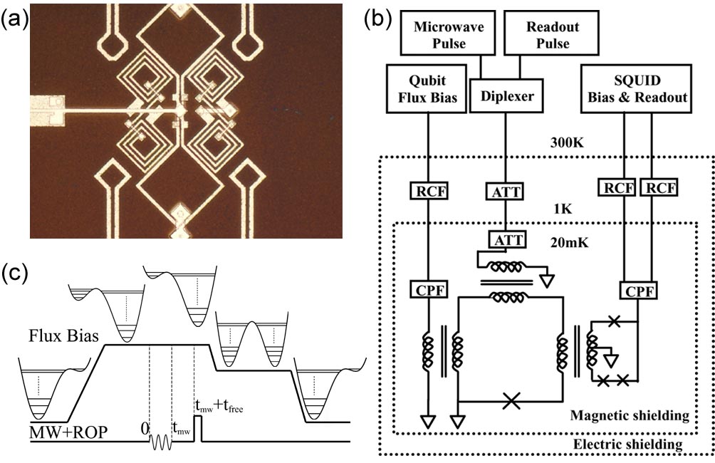
Figure 1: (Color online)(a) SEM of the sample which is fabricated by Al/AlOx/Al trilayers. (b) Schematic of the qubit circuitry. Josephson junctions are denoted by the X symbols. (c) A time profile of manipulation and measurement. The corresponding potential energy landscape is also shown.

Entanglement can exist not only in microscopic but also in macroscopic systems such as Josephson phase qubits (JPQs) Nature.467.570 ; Nature.467.574 , which are basically current or flux biased Josephson tunnel junctions having Josephson coupling energy $E_{J}$ much greater than charging energy $E_{c}$. JPQs are essentially manufacturable atoms whose Hamiltonians can be custom designed and realized with integrated circuit fabrication technology RevModPhys.73.357 ; PhysToday ; Nature.453.1031 . This unique property makes the JPQ a good test-bed for studying fundamental issues in quantum mechanics and a promising candidate for implementing quantum information processing. In our experiment reported here a flux biased JPQ, which is a radio frequency superconducting quantum interference device consisting of a superconducting loop of inductance $L\approx 770$ pH interrupted by a $4.8$ $\mu$m² Josephson junction of capacitance $C\approx 240$ fF and critical current $I_{c}\approx 1.4$ $\mu$A, is used as shown in Fig. 1(a). The two lowest levels in the upper well of the strongly tilted double well potential form the two computational basis states $|0\rangle$ and $|1\rangle$. The energy level spacing, $\omega_{10}$ (for convenience we set $\hbar\equiv h/2\pi=1$ where $h$ is Planck’s constant), between the two basis states can be continuously tuned by varying the amount of magnetic flux inductively coupled to the superconducting loop. Although atomic size defects in tunnel barrier of the Josephson junction, which are essentially microscopic two-level systems (TLSs), are considered as one of the major sources of energy relaxation and decoherence in JQP PhysRevLett.93.077003 ; PhysRevLett.95.210503 , they also have the potential to be utilized as a useful resource for quantum information processing PhysRevLett.97.077001 ; NaturePhysics.4.523 ; Nat.Commun. ; NJP2 ; PhysRevB.83.180507 . In this work, we used a TLS coupled to a JPQ to investigate the dynamics of entanglement of the coupled bipartite system. We show that for a bipartite system described by Hamiltonian (1) the degree of entanglement, quantified by “concurrence” PhysRevLett.80.2245 , in both driven and free evolution states can be obtained by measuring the state of JPQ alone, which is quite different from the conventional tomography method in studying the entanglement. The results clearly show that resonant ac drive and always-on qubit-TLS interaction together generates entanglement oscillations and that in the subsequent free evolution the system may exhibit DEO, ESD, and ESDR depending on the specific bipartite states at the time of turning off the ac drive. A comparison between the experimental results obtained with finite relaxation and decoherence and the predictions based on analytical solution of the corresponding pure states (i.e., relaxation and decoherence free) clearly shows that not only the system-environment interaction but also the bipartite system’s initial states play important roles in determining the dynamic behavior of this type of open quantum systems.

II EXPERIMENT

Fig. 1(b) shows the schematics of the circuitry used. To distinguish qubit states from those of TLS, we denote the ground and excited states of the qubit (TLS) as $|0\rangle$ $(|g\rangle)$ and $|1\rangle$ $(|e\rangle)$, respectively. The coupled qubit-TLS in a weak microwave field is described by a four-level coupled bipartite system whose effective Hamiltonian, in the basis of the four product states $\left\{\left|0g\right\rangle,\left|1g\right\rangle,\left|0e\right\rangle,\left|1e\right\rangle\right\}$, is

$$H=\left(\begin{smallmatrix}E_{0g}&\Omega_{\text{m}}\cos\omega t&0&0\\ \Omega_{\text{m}}\cos\omega t&E_{1g}&g&0\\ 0&g&E_{0e}&\Omega_{\text{m}}\cos\omega t\\ 0&0&\Omega_{\text{m}}\cos\omega t&E_{1e}\end{smallmatrix}\right),$$ (1)

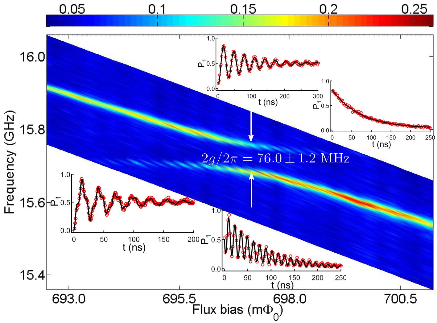
Figure 2: (Color online)Spectroscopy of the coupled qubit and TLS versus flux bias. The splitting due to the coupling between the qubit and TLS is $2g/2\pi=76.0\pm 1.2$ MHz at $f=15.722$ GHz. The inserts are Rabi oscillation, $T_{1}$, Rabi beating and vacuum Rabi oscillation, separately (from top to bottom).

where the diagonal elements are the energies of corresponding product states, $\Omega_{\text{m}}$ is the Rabi frequency of the JPQ, $g$ characterizes the qubit-TLS coupling strength, and $\omega$ is the frequency of the microwave field. Notice that at the degeneracy point one has $E_{1g}=E_{0e}$.The system’s parameters in Hamiltonian (1) were determined from spectroscopy ($2g/2\pi=76.0$ $\pm 1.2$ MHz), Rabi oscillation ($\Omega_{\text{m}}/2\pi=63.0$ MHz), pump-probe ($T_{1}^{q}\approx 61$ ns), and pump-SWAP-delay-SWAP-probe ($T_{1}^{TLS}\approx 146$ ns) experiments Nat.Commun. as shown in Fig. 2.

To measure dynamics of the coupled system, we first prepare the system in the ground state $|0g\rangle$ at $t\leq 0$, followed by applying a resonant microwave pulse of width $t_{\text{mw}}$ at $t=0$ to coherently transfer the system from $|0g\rangle$ to other states through qubit-microwave coupling $\Omega_{\text{m}}$ and qubit-TLS coupling $g.$ After the pulse is terminated at $t=t_{\text{mw}}$, the probability of finding the qubit in the state $|1\rangle$, $P_{1}=P_{1g}+P_{1e},$ is measured after a time $t_{\text{free}}$ is elapsed from the end of the microwave pulse as shown in Fig. 1(c). The procedure is repeated for different $t_{\text{mw}}$ and $t_{\text{free}}$ to obtain $P_{1}$ as a function of $t_{\text{mw}}$ and free evolution time $t_{\text{free}}$.

III RESULTS AND DISCUSSION

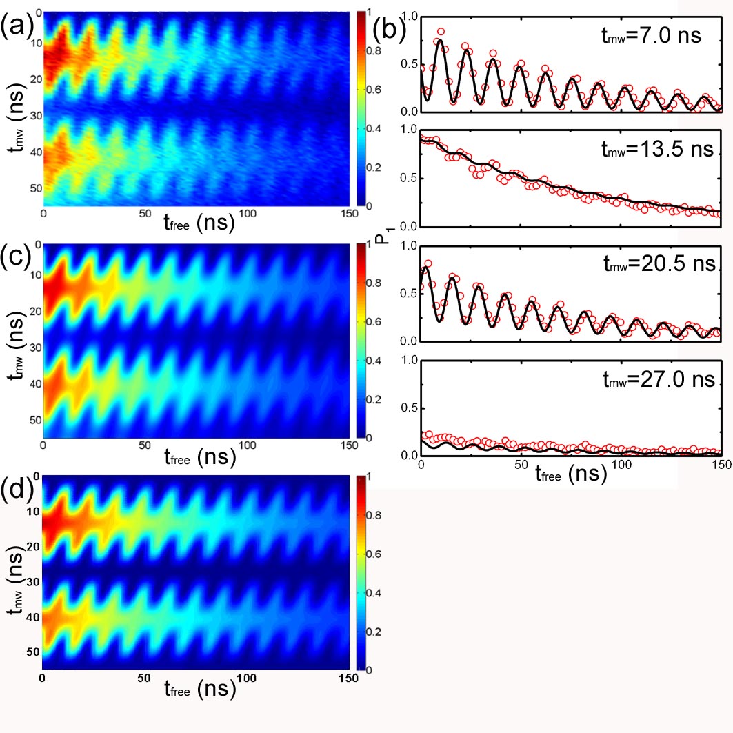
Figure 3: (Color online)(a) Experimentally measured $P_{1}$ versus $\mbox{t}_{\mathrm{mw}}$ and $\mbox{t}_{\mathrm{free}}$. (b) $P_{1}$ oscillation with typical $\mbox{t}_{\mathrm{mw}}$. The symbols are the experimental measured $P_{1}$ and the lines are numerical result. (c) Numerical result of $P_{1}$ versus $\mbox{t}_{\mathrm{mw}}$ and $\mbox{t}_{\mathrm{free}}$. (d) Analytical result of $P_{1}$ versus $\mbox{t}_{\mathrm{mw}}$ and $\mbox{t}_{\mathrm{free}}$.

To facilitate a direct comparison to analytical result in our experiment the qubit-TLS was biased at the center of the anticrossing where $E_{1g}=E_{0e}$. Fig. 3(a) shows the complete set of $P_{1}(t_{\text{mw}},t_{\text{free}})$ data measured. To clearly illustrate the effect of $t_{\text{mw}}$ on vacuum Rabi oscillation of $P_{1}$ at $t\geq t_{\text{mw}},$ data taken with $t_{\text{mw}}=7.0,13.5,20.5$, and $27.0$ ns are plotted as symbols in Fig. 3(b). Notice that while the initial phase of $P_{1}$ oscillation depends on $t_{\text{mw}}$ the frequency is independent of $t_{\text{mw}}$ and its value, $76$ MHz, agrees very well with the size of the splitting $2g$ obtained from the spectroscopic measurement. Furthermore, the data with $t_{\text{mw}}=13.5$ ns and $t_{\text{mw}}=27.0$ ns show very little oscillation while in a stark contrast the data with $t_{\text{mw}}=7.0$ ns and $t_{\text{mw}}=20.5$ ns oscillate with much larger amplitudes. Their oscillations are out of phase with each other indicating the importance of initial phase of vacuum Rabi oscillation in determining concurrence as discussed below.

To understand the dynamics of this coupled bipartite quantum system, we first discuss the ideal situation of pure state evolution by solving the problem analytically. In rotating frame Hamiltonian (1) is transformed to:

$$H_{r}=\left(\begin{smallmatrix}0&\frac{\Omega_{\text{m}}}{2}\theta(t_{\text{mw}}-t)&0&0\\ \frac{\Omega_{\text{m}}}{2}\theta(t_{\text{mw}}-t)&0&g&0\\ 0&g&0&\frac{\Omega_{\text{m}}}{2}\theta(t_{\text{mw}}-t)\\ 0&0&\frac{\Omega_{\text{m}}}{2}\theta(t_{\text{mw}}-t)&0\end{smallmatrix}\right),$$ (2)

where $\theta(t_{\text{mw}}-t)$ is the heaviside step function with $\theta(t_{\text{mw}}-t)=1$ for $t<t_{\text{mw}}$ and $\theta(t_{\text{mw}}-t)=0$ for $t>t_{\text{mw}}$. It is obvious from Hamiltonian (2) that the dynamics occurs only in the subspace $\{|1g\rangle,|0e\rangle\}$ for $t>t_{\text{mw}}$. Writing the wavefunction of the system in the form $|\Psi(t)\rangle=c_{0g}(t)|0g\rangle+c_{1g}(t)|1g\rangle+c_{0e}(t)|0e\rangle+c_{1e}(t)|1e\rangle$, we obtain probability amplitudes by solving the time dependent Schrödinger equation directly. For $t\leqslant t_{\text{mw}}$, we have

$$c_{0g}(t) =\frac{1}{\Omega_{\text{m}}^{2}+\Omega_{+}^{2}}\left[\Omega_{\text{m}}^{2}\cos(\Omega_{+}t/2)+\Omega_{+}^{2}\cos(\Omega_{-}t/2)\right],$$

$$c_{1g}(t) =-i\frac{\Omega_{m}\Omega_{+}}{\Omega_{\text{m}}^{2}+\Omega_{+}^{2}}[\sin(\Omega_{+}t/2)+\sin(\Omega_{-}t/2)]$$

$$=-i\frac{2\Omega_{\text{m}}\Omega_{+}}{\Omega_{\text{m}}^{2}+\Omega_{+}^{2}}\sin\frac{\Omega_{\text{s}}t}{2}\cos\frac{gt}{2},$$

$$c_{0e}(t) =\frac{\Omega_{\text{m}}\Omega_{+}}{\Omega_{\text{m}}^{2}+\Omega_{+}^{2}}[\cos(\Omega_{+}t/2)-\cos(\Omega_{-}t/2)]$$ (3)

$$=-\frac{2\Omega_{\text{m}}\Omega_{+}}{\Omega_{\text{m}}^{2}+\Omega_{+}^{2}}\sin\frac{\Omega_{\text{s}}t}{2}\sin\frac{gt}{2},$$

$$c_{1e}(t) =\frac{-i}{\Omega_{\text{m}}^{2}+\Omega_{+}^{2}}\left[\Omega_{\text{m}}^{2}\sin(\Omega_{+}t/2)-\Omega_{+}^{2}\sin(\Omega_{-}t/2)\right],$$

with $\Omega_{+}=\Omega_{\text{s}}+g$, $\Omega_{-}=\Omega_{\text{s}}-g$, and $\Omega_{\text{s}}=\sqrt{\Omega_{\text{m}}^{2}+g^{2}}$. Notice that the quantity measured directly in our experiment, $P_{1}(t)=|c_{1g}(t)|^{2}+|c_{1e}(t)|^{2},$ undergoes anomalous Rabi oscillation which in general contains all three frequency components $\Omega_{+}$, $\Omega_{-}$, and $\Omega_{\text{s}}$.

When the system is driven by a resonant microwave field $P_{2}(t<t_{\text{mw}})$, being the probability of finding the system in the subspace spanned by $|1g\rangle$ and $|0e\rangle$, undergoes sinusoidal oscillation:

$$P_{2}(t\leq t_{\text{mw}})=|c_{1g}|^{2}+|c_{0e}|^{2}=\frac{2\Omega_{\text{m}}^{2}\Omega_{+}^{2}}{(\Omega_{\text{m}}^{2}+\Omega_{+}^{2})^{2}}(1-\cos\Omega_{\text{s}}t),$$ (4)

which shows that amplitude of the oscillation depends only on the ratio $g/\Omega_{\text{m}}$. In our experiment, $g/\Omega_{\text{m}}\simeq 0.60$ yielding $P_{2\max}\simeq 0.74$ which agrees well with the experiment.

For $t>t_{\text{mw}}$, $t_{\text{free}}=t-t_{\text{mw}}$, it is straightforward to show

$$c_{0g}(t) =c_{0g}(t_{\text{mw}})$$

$$c_{1g}(t) =\cos gt_{\text{free}}\cdot c_{1g}(t_{\text{mw}})-i\sin gt_{\text{free}}\cdot c_{0e}(t_{\text{mw}})$$

$$c_{0e}(t) =\cos gt_{\text{free}}\cdot c_{0e}(t_{\text{mw}})-i\sin gt_{\text{free}}\cdot c_{1g}(t_{\text{mw}})$$

$$c_{1e}(t) =c_{1e}(t_{\text{mw}}).$$

In this case, the probability of finding the qubit in sate $|1\rangle$ can be expressed as

$$\begin{split}P_{1}(t&>t_{\text{mw}})=|c_{\text{1e}}|^{2}+|c_{\text{1g}}|^{2}\\ &=P_{1e}(t_{\text{mw}})+\frac{1}{2}P_{2}(t_{\text{mw}})(1+\cos(2gt_{\text{free}}+gt_{\text{mw}})),\end{split}$$ (5)

with $P_{1e}(t_{\text{mw}})=|c_{1e}(t_{\text{mw}})|^{2}$ being the population of $|1e\rangle$ and $P_{2}(t_{\text{mw}})\equiv P_{1g}(t_{\text{mw}})+P_{0e}(t_{\text{mw}})=\frac{4\Omega_{\text{m}}^{2}\Omega_{+}^{2}}{(\Omega_{\text{m}}^{2}+\Omega_{+}^{2})^{2}}\sin^{2}\frac{\Omega_{\text{s}}t_{\text{mw}}}{2}$ being the probability of finding the system in the subspace spanned by $|1g\rangle$ and $|0e\rangle$ at $t=t_{\text{mw}}$ which remains constant for $t>t_{\text{mw}}$. Eq. (5) shows that after microwave is turned off the system undergoes vacuum Rabi oscillation caused by the interaction between $|1g\rangle$ and $|0e\rangle.$ The angular frequency, depth (peak-to-peak), initial phase, and bottom envelope of the oscillation are $2g$, $P_{2}(t_{\text{mw}})$, $gt_{\text{mw}}$, and $P_{1e}(t_{\text{mw}})$, respectively. In addition, because $P_{0g}(t_{\text{mw}})+P_{2}(t_{\text{mw}})+P_{1e}(t_{\text{mw}})=1$ the difference between unity and the top envelope of $P_{1}(t_{\text{mw}},t_{\text{free}})$ is just $P_{0g}(t_{\text{mw}})$.

Interestingly, when $\Omega_{\text{s}}t_{\text{mw}}=2n\pi$, $P_{2}(t_{\text{mw}})=0$, i.e., vacuum Rabi oscillation vanishes and one has

$$P_{1}(t_{\text{mw}},t_{\text{free}})=\sin^{2}\frac{gt_{\text{mw}}}{2},$$ (6)

which is independent of $t_{\text{free}}$. In addition, if $\Omega_{+}t_{\text{mw}}\simeq(2k+1)\pi$, one has $P_{1}\simeq 1$, which corresponds to the population mainly occupying $|1e\rangle$; if $\Omega_{+}t_{\text{mw}}\simeq 2k\pi$ , one has $P_{1}\simeq 0$, which corresponds to the population mainly occupying $|0g\rangle$. These two cases correspond to $t_{\text{mw}}=13.5$ ns and $27.0$ ns, respectively, as shown in Fig. 3(b) where the exponential decay is due to energy relaxation.

Although the basic physics is the same, because of decoherence and relaxation the experimental system investigated here cannot be represented by pure states but mixed states described by the bipartite density operator $\mathbf{\rho}\left(t\right)$. The diagonal matrix elements $\rho_{mm}$ and off-diagonal matrix elements $\rho_{mn}$ $(m\neq n)$ represent the occupation probability of the state $\left|m\right\rangle$ and coherence between the states $\left|m\right\rangle$ and $\left|n\right\rangle$, respectively. To simulate the system’s dynamics, we solve the master equation zhou1 ; Gardiner

$$\frac{d\rho_{mn}}{dt}=\sum_{m^{\prime}n^{\prime}}(-iL_{mn,m^{\prime}n^{\prime}}+R_{mn,m^{\prime}n^{\prime}})\rho_{m^{\prime}n^{\prime}},$$ (7)

where, $L_{mn,m^{\prime}n^{\prime}}=\left[H_{mm^{\prime}}\delta_{n^{\prime}n}-H_{n^{\prime}n}\delta_{mm^{\prime}}\right],$ $H_{mm^{\prime}}$ is matrix element of the system’s Hamiltonian, and $R_{mn,m^{\prime}n^{\prime}}$ is the damping rate matrix element whose value is proportional to the energy relaxation rate zhou1 . Eq. (7) is numerically integrated to obtain $\mathbf{\rho}\left(t\right).$ The results is shown in Fig. 3(c) as well as the solid lines in Fig. 2 (resonant ac drive) and Fig. 3(b) (free evolution). It can be seen clearly from Fig. 2 that unlike the normal sinusoidal Rabi oscillation observed in the region of large qubit-TLS detuning, at the degeneracy point the oscillation of $P_{1}(t\leq t_{\text{mw}})$ is clearly non-sinusoidal due to more complicated dynamics of the driven four-level system NJP_Ashhab ; PhysRevB.80.172506 ; PhysRevB.81.100511 ; PhysRevB.82.132501 . In Fig. 3(d) we also show the calculated $P_{1}$ based on the analytical solution Eq. (5) by treating the effect of energy relaxation phenomenologically. Notice that agreement between the experimental, numerical, and analytical results in the entire range of driven and free evolution is very good confirming quantitative understanding of the system’s dynamics.

To study the dynamics of qubit-TLS entanglement, we examine how concurrence, denoted as $C_{\rho}$ PhysRevLett.80.2245 for mixed states, evolves with time. In Fig. 4(a) $C_{\rho}$ derived from the measured $P_{1}$ is shown. Of particular interest is that $C_{\rho}$ is observed to undergo damped oscillation in both of the driven and free run (i.e., autonomous) parts of the evolution. Fig. 4(c) shows the Rabi-like oscillation when the system is driven by the resonant microwave field. The corresponding $C_{\rho}$ (the dashed line) oscillates and undergoes sudden death and revival repeatedly. The extrema of $C_{\rho}$ are correlated strongly with the distinctive “shoulder” feature in $P_{1}.$ Fig. 4(b) shows $C_{\rho}$ in the free run part of the system’s evolution with $t_{\text{mw}}=7.0,13.5,20.5,$ and $27.0$ ns, respectively. When $t_{\text{mw}}=7.0$ ns and $t_{\text{mw}}=20.5$ ns, the qubit and TLS are mostly in $\{|1g\rangle$ and $|0e\rangle\}$. The coupling between these two basis states via the $g(|1g\rangle\langle 0e|+|0e\rangle\langle 1g|)$ term of the system Hamiltonian thus leads to time-dependent entanglement causing $C_{\rho}$ to oscillate. In this case, the entanglement dynamics clearly exhibits the phenomena of no ESD (NESD) and ESDR TingYu01302009 , respectively. In contrast, when $t_{\text{mw}}=27.0$ ns ($t_{\text{mw}}=13.5$ ns), the system is mostly in $|0g\rangle$ ($|1e\rangle$), which is decoupled from all other three basis states after microwave was turned off (neglecting energy relaxation). This results in a weak entanglement characterized by a small overall value of concurrence $C_{\rho}$ at the start of free evolution and, when decoherence is taken in account, the entanglement sudden death.

Further insights into this type of system’s entanglement dynamics and the effects of environment can be obtained by examining time-dependent concurrence of the corresponding pure state system and comparing it with the experimental result. For the corresponding pure states, concurrence $\mathcal{C}=2|c_{0g}c_{1e}-c_{1g}c_{0e}|$ William2001 . From Eq. (3), we obtain

$$\begin{split}\mathcal{C}&=|\frac{1}{(\Omega_{\text{m}}^{2}+\Omega_{+}^{2})^{2}}[\Omega_{\text{m}}^{4}\sin\Omega_{+}t_{\text{mw}}-\Omega_{+}^{4}\sin\Omega_{-}t_{\text{mw}}\\ &+2\Omega_{\text{m}}^{2}\Omega_{+}^{2}\sin gt_{\text{mw}}]+P_{2}(t_{\text{mw}})\sin(2gt_{\text{free}}+gt_{\text{mw}})|\\ &\equiv|f(\Omega_{\text{m}},g,t_{\text{mw}})+P_{2}(t_{\text{mw}})\sin(2gt_{\text{free}}+gt_{\text{mw}})|.\end{split}$$ (8)

Eq. (8) shows that when driven by a resonant microwave field entanglement oscillation is rather complex which has three frequency components $\Omega_{+},$ $\Omega_{-},$ and $g.$ In the free evolution stage the so called preconcurrence PhysRevLett.80.2245 , which is the quantity inside the absolute value sign of Eq. (8), undergoes sinusoidal oscillation with amplitude $P_{2}(t_{\text{mw}}),$ which can be obtained directly from measured $P_{1}(t_{\text{mw}},t_{\text{free}})$ according to Eq. (5), and a vertical offset $|f(\Omega_{\text{m}},g,t_{\text{mw}})|$. Hence, concurrence exhibits the ”high-low” oscillation shown in Fig.4(b) unless offset of preconcurrence is zero. By varying $t_{\text{mw}}$ and measuring the subsequent vacuum Rabi oscillation one can trace time evolution of concurrence of the driven as well as the autonomous stage of evolution. The result also shows that measuring the state of phase qubit alone is sufficient to gain all information about entanglement dynamics of this bipartite system.

In particular, when $\Omega_{\text{s}}t_{\text{mw}}=2n\pi$ one has $P_{2}(t_{\text{mw}})=0$ as discussed above and thus only $|0g\rangle$ and $|1e\rangle$ contribute to concurrence:

$$\mathcal{C}=2|c_{0g}c_{1e}|=2\sqrt{P_{1}(1-P_{1})}=|\sin gt_{\text{mw}}|,$$ (9)

which is independent of $t_{\text{free}}$. In addition, when $gt_{\text{mw}}\simeq(2k+1)\pi$ and $gt_{\text{mw}}\simeq 2k\pi$, where $k$ is an integer, we have $\mathcal{C}\ll 1$ [notice the different vertical scales in Fig.4(b)] because either $P_{1}\simeq 1$ or $P_{1}\simeq 0$.

According to Eq. (8), for pure states the amplitude of concurrence oscillation remains constant for all $t$ and $\mathcal{C}$ reaches zero at a discrete set of times only as shown in the insets of Fig. 4(b). In contrast, the experimental result displays a variety of interesting behaviors including DEO, ESD, and ESDR illustrated in Fig. 4(b) (from top to bottom). Because the main difference between the measured qubit-TLS system and the corresponding hypothetical pure state system is that the former is an open quantum system interacting with its environment (e.g., energy relaxation and decoherence) while the latter is isolated, our result shows that environment is the dominant mechanism of the observed complex entanglement dynamicsQuantumInfProcess.8.535 .

IV CONCLUSION

In summary, we have experimentally demonstrated that the coupled qubit-TLS system is a test bed for quantitatively studying the dynamics of bipartite entanglement. The measured time evolutions of this bipartite system, either when driven by a resonant microwave field or in free evolution, agree very well with the analytical and numerical solutions. Our results demonstrate that in situations similar to those described here one not only can quantify entanglement via concurrence by measuring the state of one constituent only, but also be able to control the dynamics of the entanglement by adjusting the interaction time between the qubit and the ac resonant driving field. A comparison between the temporal evolutions of concurrence of the open and the corresponding isolated systems indicates that for the bipartite system studied here the entanglement oscillation and revival are originated from the qubit-TLS coupling while the entanglement decay and sudden death are due to the coupling to the environment.

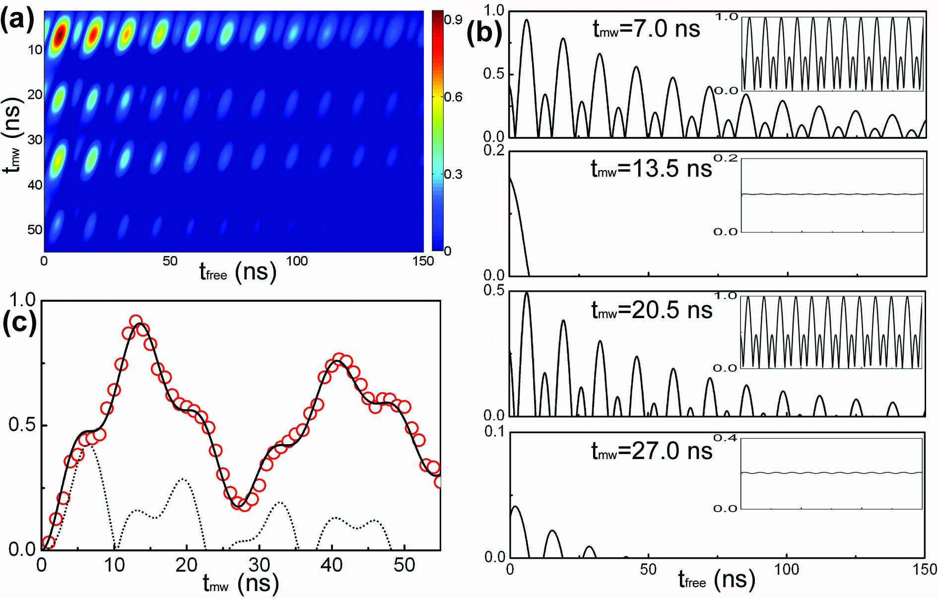
Figure 4: (Color online)(a) Concurrence as a function of $\mbox{t}_{\mathrm{mw}}$ and $\mbox{t}_{\mathrm{free}}$ extracted from the experimental data. (b) Concurrence with $\mbox{t}_{\mathrm{mw}}$=7.0, 13.5, 20.5, and 27.0 ns, respectively. Analytical results of concurrence without decoherence are shown in the insets. Notice that the different vertical scales are used. (c) $P_{1}$ and concurrence as a function of $\mbox{t}_{\mathrm{mw}}$. Open circles are experimental data and the solid line is the numerical result of $P_{1}$. The dashed line is the corresponding concurrence.

- (1) E. Schrödinger, Naturwissenschaften 23, 807 (1935).
- (2) A. Einstein, B. Podolsky, B. and N. Rosen, Phys. Rev. 47, 777 (1935).
- (3) J.-S. Xu, X.-Y. Xu, C.-F.Li, C.-J. Zhang, X.-B. Zou, and G.-C. Guo, Nature Communications 1, 7 (2010).
- (4) Y. Hu and L. Tian, Phys. Rev. Lett. 106, 257002 (2011).
- (5) F. Minterta, A. R. R. Carvalhoa, M. Kuś and A. Buchleitner, Phys. Rep. 415, 207 (2005).
- (6) L. Amico, R. Fazio, A. Osterloh and V. Vedral, Rev. Mod. Phys. 80, 517 (2008).
- (7) R. Horodecki, P. Horodecki, M. Horodecki and K. Horodecki, Rev. Mod. Phys. 81, 865 (2009).
- (8) M. Neeley, R. C. Bialczak, M. Lenander, E. Lucero, M. Mariantoni, A. D. O’Connell, D. Sank, H. Wang, M. Weides, J. Wenner, Y. Yin, T. Yamamoto, A. N. Cleland and J. M. Martinis, Nature 467, 570 (2010).
- (9) L. DiCarlo, M. D. Reed, L. Sun, B. R. Johnson, J. M. Chow, J. M. Gambetta, L. Frunzio, S. M. Girvin, M. H. Devoret and R. J. Schoelkopf, Nature 467,574 (2010).
- (10) Y. Makhlin, G. Schön, A. Shnirman, Rev. Mod. Phys. 73, 357 (2001).
- (11) J. You and F. Nori, Physics Today 58(11), 42 (2005).
- (12) J. Clarke and F. K. Wilhelm, Nature 453, 1031 (2008).
- (13) R. W. Simmonds, K. M. Lang, D. A. Hite, S. Nam, D. P. Pappas, and J. M. Martinis, Phys. Rev. Lett. 93, 077003 (2004).
- (14) J. M. Martinis, K. B. Cooper, R. McDermott, M. Steffen, M. Ansmann, K. D. Osborn,K. Cicak, S. Oh, D. P. Pappas, R. W. Simmonds, C. C. Yu, Phys. Rev. Lett. 95, 210503 (2005).
- (15) A. M. Zagoskin, S. Ashhab, J. R. Johansson and F. Nori et al., Phys. Rev. Lett. 97, 077001 (2006).
- (16) M. Neeley, M. Ansmann, R. C. Bialczak, M. Hofheinz, E. L. N. Katz, A. O’Connell, H. Wang, A. N. Cleland and J. M. Martinis, Nature Physics 4, 523 (2008).
- (17) G. Sun, X. Wen, B. Mao, J. Chen, Y. Yu, P. Wu and S. Han, Nature Communications 1, 51 (2010).
- (18) G. J. Grabovskij, P. Bushev, J. H. Cole, C. Müller, J. Lisenfeld, A. Lukashenko and A. V. Ustinov, New J. Phys. 13, 063015 (2011).
- (19) G. Sun, X. Wen, B. Mao, Y. Yu, J. Chen, W. Xu, L. Kang, P. Wu and S. Han, Phys. Rev. B 83, 180507(R) (2011).
- (20) W. K. Wootters, Phys. Rev. Lett. 80, 2245 (1998).
- (21) Z. Zhou, S.-I. Chu and S. Han, J. Phys. B: At. Mol. Opt. Phys. 41, 045506 (2008).
- (22) G. W. Gardiner and P. Zoller, Quantum Noise (Springer Verlag, Berlin, 2004), 3rd ed.
- (23) S. Ashhab, J. R. Johansson and F. Nori, New J. Phys. 8, 103 (2006).
- (24) A. Lupaşcu, P. Bertet, E. F. C. Driessen, C. J. P. M. Harmans and J. E. Mooij, Phys. Rev. B 80, 172506 (2009).
- (25) J. Lisenfeld, C. Müller, J. H. Cole, P. Bushev, A. Lukashenko, A. Shnirman, and A. V. Ustinov, Phys. Rev. B 81, 100511(R) (2010).
- (26) G. Sun, X. Wen, B. Mao, Z. Zhou, Y. Yu, P. Wu, S. Han, Phys. Rev. B 82, 132501 (2010).
- (27) T. Yu and J. H. Eberly, Science 323, 598 (2009).
- (28) W. K. Wootters, Quantum Inf. and Compt. 1, 27 (2001).
- (29) J. P. Paz and A. J. Roncaglia, Quantum Inf. Process. 8, 535 (2009).