Down the Rabbit Hole: Robust Proximity Search and Density Estimation in Sublinear Space

Abstract

For a set of $n$ points in ${\rm I\!R}^{d}$, and parameters $k$ and ${\varepsilon}$, we present a data structure that answers $(1+{\varepsilon},k)$-ANN queries in logarithmic time. Surprisingly, the space used by the data-structure is $\widetilde{O}(n/k)$; that is, the space used is sublinear in the input size if $k$ is sufficiently large. Our approach provides a novel way to summarize geometric data, such that meaningful proximity queries on the data can be carried out using this sketch. Using this, we provide a sublinear space data-structure that can estimate the density of a point set under various measures, including: (i) sum of distances of $k$ closest points to the query point, and (ii) sum of squared distances of $k$ closest points to the query point. Our approach generalizes to other distance based estimation of densities of similar flavor.

We also study the problem of approximating some of these quantities when using sampling. In particular, we show that a sample of size $\widetilde{O}(n/k)$ is sufficient, in some restricted cases, to estimate the above quantities. Remarkably, the sample size has only linear dependency on the dimension.

1 Introduction

Given a set $\mathsf{P}$ of $n$ points in ${\rm I\!R}^{d}$, the nearest neighbor problem is to construct a data structure, such that for any query point $\mathtt{q}$ it (quickly) finds the closest point to $\mathtt{q}$ in $\mathsf{P}$. This is an important and fundamental problem in Computer Science [SDI06, Cha08, AI08, Cla06]. Applications of nearest neighbor search include pattern recognition [FH49, CH67], self-organizing maps [Koh01], information retrieval [SWY75], vector compression [GG91], computational statistics [DW82], clustering [DHS01], data mining, learning, and many others. If one is interested in guaranteed performance and near linear space, there is no known way to solve this problem efficiently (i.e., logarithmic query time) for dimension $d>2$.

A commonly used approach for this problem is to use Voronoi diagrams. The Voronoi diagram of $\mathsf{P}$ is the decomposition of ${\rm I\!R}^{d}$ into interior disjoint closed cells, so that for each cell $C$ there is a unique single point $\mathsf{p}\in\mathsf{P}$ such that for any point $\mathtt{q}\in\mathrm{int}\!\left({C}\right)$ the nearest-neighbor of $\mathtt{q}$ in $\mathsf{P}$ is $\mathsf{p}$. Thus, one can compute the nearest neighbor of $\mathtt{q}$ by a point location query in the collection of Voronoi cells. In the plane, this approach leads to $O(\log n)$ query time, using $O(n)$ space, and preprocessing time $O(n\log n)$. However, in higher dimensions, this solution leads to algorithms with exponential dependency on the dimension. The complexity of a Voronoi diagram of $n$ points in ${\rm I\!R}^{d}$ is $\Theta\left({n^{\left\lceil{d/2}\right\rceil}}\right)$ in the worst case. By requiring slightly more space, Clarkson [Cla88] showed a data-structure with query time $O\!\left({\log n}\right)$, and $O\!\left({n^{\left\lceil{d/2}\right\rceil+\delta}}\right)$ space, where $\delta>0$ is a prespecified constant (the $O(\cdot)$ notation here hides constants that are exponential in the dimension). One can tradeoff the space used and the query time [AM93]. Meiser [Mei93] provided a data-structure with query time $O\!\left({d^{5}\log n}\right)$ (which has polynomial dependency on the dimension), where the space used is $O\!\left({n^{d+\delta}}\right)$. Therefore, even for moderate dimension, the exact nearest neighbor data-structure uses an exorbitant amount of storage. It is believed that there is no efficient solution for the nearest neighbor problem when the dimension is sufficiently large [MP69]; this difficulty has been referred to as the “curse of dimensionality”.

Approximate Nearest Neighbor (ANN).

In light of the above, major effort has been devoted to develop approximation algorithms for nearest neighbor search [AMN⁺98, IM98, KOR00, SDI06, Cha08, AI08, Cla06, HIM12]. In the $(1+{\varepsilon})$-approximate nearest neighbor problem (the ANN problem), one is additionally given an approximation parameter ${\varepsilon}>0$ and one is required to find a point $\mathsf{u}\in\mathsf{P}$ such that $\left\lVert{{\mathtt{q}}-{\mathsf{u}}}\right\rVert\leq(1+{\varepsilon})\mathsf{d}\!\left({\mathtt{q},\mathsf{P}}\right)$. In $d$ dimensional Euclidean space, one can answer ANN queries, in $O(\log n+1/{\varepsilon}^{d-1})$ time using linear space [AMN⁺98, Har11]. Because of the $1/{\varepsilon}^{d-1}$ in the query time, this approach is only efficient in low dimensions. Interestingly, for this data-structure, the approximation parameter ${\varepsilon}$ need not be specified during the construction, and one can provide it during the query. An alternative approach is to use Approximate Voronoi Diagrams (AVD), introduced by Har-Peled [Har01], which is a partition of space into regions of low total complexity, with a representative point for each region, that is an ANN for any point in the region. In particular, Har-Peled showed that there is such a decomposition of size $O\!\left({(n/{\varepsilon}^{d})\log^{2}n}\right)$, see also [HIM12]. This allows ANN queries to be answered in $O(\log n)$ time. Arya and Malamatos [AM02] showed how to build AVDs of linear complexity (i.e., $O(n/{\varepsilon}^{d})$). Their construction uses WSPD (Well Separated Pair Decomposition) [CK95]. Further tradeoffs between query time and space usage for AVDs were studied by Arya et al. [AMM09].

$k$-nearest neighbor.

A more general problem is the $k$-nearest neighbors problem where one is interested in finding the $k$ points in $\mathsf{P}$ nearest to the query point $\mathtt{q}$. This is widely used in pattern recognition, where the majority label is used to label the query point. In this paper, we are interested in the more restricted problem of approximating the distance to the $k$th nearest neighbor and finding a data point achieving the approximation. We call this problem the $(1+{\varepsilon},k)$-approximate nearest neighbor ($(1+{\varepsilon},k)$-ANN) problem. This problem is widely used for density estimation in statistics, with $k\approx\sqrt{n}$ [Sil86]. It is also used in meshing (with $k=2d$), or to compute the local feature size of a point set in ${\rm I\!R}^{d}$ [Rup95]. The problem also has applications in non-linear dimensionality reduction; finding low dimensional structures in data – more specifically low dimensional submanifolds embedded in Euclidean spaces. Algorithms like ISOMAP, LLE, Hessian-LLE, SDE and others, use the $k$-nearest neighbor as a subroutine [Ten98, BSLT00, MS94, WS06].

Density estimation.

Given distributions $\mu_{1},\ldots,\mu_{k}$ defined over ${\rm I\!R}^{d}$, and a query point $\mathtt{q}$, we want to compute the a posteriori probabilities of $\mathtt{q}$ being generated by one of these distributions. This approach is used in unsupervised learning as a way to classify a new point. Naturally, in most cases, the distributions are given implicitly; that is, one is given a large number of points sampled from each distribution. So, let $\mu$ be such a distribution, and $\mathsf{P}$ be a set of $n$ samples. To estimate the density of $\mu$ at $\mathtt{q}$, a standard Monte Carlo technique is to consider a ball $\mathsf{B}$ centered at $\mathtt{q}$, and count the number of points of $\mathsf{P}$ inside $\mathsf{B}$. Specifically, one possible approach that is used in practice [DHS01], is to find the smallest ball centered at $\mathtt{q}$ that contains $k$ points of $\mathsf{P}$ and use this to estimate the density of $\mu$. The right value of $k$ has to be chosen carefully – if it is too small, then the estimate is unstable (unreliable), and if it is too large, it either requires the set $\mathsf{P}$ to be larger, or the estimate is too “smoothed” out to be useful (values of $k$ that are used in practice are $\widetilde{O}(\sqrt{n})$), see Duda et al. [DHS01] for more details. To do such density estimation, one needs to be able to answer, approximate or exact, $k$-nearest neighbor queries.

Sometimes one is interested not only in the radius of this ball centered at the query point, but also in the distribution of the points inside this ball. The average distance of a point inside the ball to its center, can be estimated by the sum of distances of the sample points inside the ball to the center. Similarly, the variance of this distance can be estimated by the sum of squared distances of the sample points inside the ball to the center of the ball. As mentioned, density estimation is used in manifold learning and surface reconstruction. For example, Guibas et al. [GMM11] recently used a similar density estimate to do manifold reconstruction.

Answering exact $k$-nearest neighbor queries.

Given a point set $\mathsf{P}\subseteq{\rm I\!R}^{d}$, computing the partition of space into regions, such that the $k$ nearest neighbors do not change, is equivalent to computing the $k$th order Voronoi diagram. Via standard lifting, this is equivalent to computing the first $k$ levels in an arrangement of hyperplanes in ${\rm I\!R}^{d+1}$ [Aur91]. More precisely, if we are interested in the $k$th-nearest neighbor, we need to compute the $(k-1)$-level in this arrangement.

The complexity of the $(\leq k)$ levels of a hyperplane arrangement in ${\rm I\!R}^{d+1}$ is $\Theta(n^{\left\lfloor{(d+1)/2}\right\rfloor}(k+1)^{\left\lceil{(d+1)/2}\right\rceil})$ [CS89]. The exact complexity of the $k$th-level is not completely understood and achieving tight bounds on its complexity is one of the long-standing open problems in discrete geometry [Mat02]. In particular, via an averaging argument, in the worst case, the complexity of the $k$th-level is $\Omega\!\left({n^{\left\lfloor{(d+1)/2}\right\rfloor}(k+1)^{\left\lceil{(d+1)/2}\right\rceil-1}}\right)$. As such, the complexity of $k$th-order Voronoi diagram is $\Omega(nk)$ in two dimensions, and $\Omega(n^{2}k)$ in three dimensions.

Thus, to provide a data-structure for answering $k$-nearest neighbor queries exactly and quickly (i.e., logarithmic query time) in ${\rm I\!R}^{d}$, requires computing the $k$-level of an arrangement of hyperplanes in ${\rm I\!R}^{d+1}$. The space complexity of this structure is prohibitive even in two dimensions (this also effects the preprocessing time). Furthermore, naturally, the complexity of this structure increases as $k$ increases. On the other end of the spectrum one can use partition-trees and parametric search to answer such queries using linear space and query time (roughly) $O\!\left({n^{1-1/(d+1)}}\right)$ [Mat92, Cha10]. One can get intermediate results using standard space/time tradeoffs [AE98].

Known results on approximate $k$-order Voronoi diagram.

Similar to AVD, one can define a AVD for the $k$-nearest neighbor. The case $k=1$ is the regular approximate Voronoi diagram [Har01, AM02, AMM09]. The case $k=n$ is the furthest neighbor Voronoi diagram. It is not hard to see that it has a constant size approximation (see [Har99], although it was probably known before). Our results (see below) can be interpreted as bridging between these two extremes.

Quorum clustering.

Carmi et al. [CDH⁺05] describe how to compute efficiently a partition of the given point set $\mathsf{P}$ into clusters of $k$ points each, such that the clusters are compact. Specifically, this quorum clustering computes the smallest ball containing $k$ points, removes this cluster, and repeats, see Section 2.2.1 for more details. Carmi et al. [CDH⁺05] also describe a data-structure that can approximate the smallest cluster. The space usage of their data structure is $\widetilde{O}(n/k)$, but it cannot be directly used for our purposes. Furthermore, their data-structure is for two dimensions and it cannot be extended to higher dimensions, as it uses additive Voronoi diagrams (which have high complexity in higher dimensions).

Our results.

We first show, in Section 3, how to build a data-structure that answers $(15,k)$-ANN queries in time $O(\log n)$, where the input is a set of $n$ points in ${\rm I\!R}^{d}$. Surprisingly, the space used by this data-structure is $O(n/k)$. This result is surprising as the space usage decreases with $k$. This is in sharp contrast to behavior in the exact version of the $k$th-order Voronoi diagram (where the complexity increases with $k$). Furthermore, for super-constant $k$ the space used by this data-structure is sublinear. For example, in some applications the value of $k$ used is $\Omega\!\left({\sqrt{n}}\right)$, and the space used in this case is a tiny fraction of the input size. This is a general reduction showing that such queries can be reduced to proximity search in an appropriate product space over $n/k$ points computed carefully.

In Section 4, we show how to construct an approximate $k$-order Voronoi diagram using space $O({\varepsilon}^{-d-1}n/k)$ (here ${\varepsilon}>0$ is an approximation quality parameter specified in advance). Using this data-structure one can answer $(1+{\varepsilon},k)$-ANN queries in $O(\log n)$ time. See Theorem 4.9 for the exact result.

General density queries.

We show in Section 5, as an application of our data-structure, how to answer more robust queries. For example, one can approximate (in roughly the same time and space as above) the sum of distances, or squared distances, from a query point to its $k$ nearest neighbors. This is useful in approximating density measures [DHS01]. Surprisingly, our data-structure can be used to estimate the sum of any function $f(\cdot)$ defined over the $k$ nearest neighbors, that depends only on the distance of these points from the query point. Informally, we require that $f(\cdot)$ is monotonically increasing with distance, and it is (roughly) not super-polynomial. For example, for any constant $p>0$, our data-structure requires sublinear space (i.e., $\widetilde{O}\!\left({n/k}\right)^{\rule[-5.69046pt]{0.0pt}{11.38092pt}}$), and given a query point $\mathtt{q}$, it can $(1+{\varepsilon})$-approximate the quantity $\sum_{\mathsf{u}\in X}\left\lVert{{\mathsf{u}}-{\mathtt{q}}}\right\rVert^{p}$, where $X$ is the set of $k$ nearest points in $\mathsf{P}$ to $\mathtt{q}$. The query time is logarithmic.

To facilitate this, in a side result, that might be of independent interest, we show how to perform point-location queries in $I$ compressed quadtrees of total size $m$ simultaneously in $O(\log m+I)$ time (instead of the naive $O(I\log m)$ query time), without asymptotically increasing the space needed.

If $k$ is specified with the query.

In Section 6, given a set $\mathsf{P}$ of $n$ points in ${\rm I\!R}^{d}$, we show how to build a data-structure, in $O(n\log n)$ time and using $O(n)$ space, such that given a query point and parameters $k$ and ${\varepsilon}$, the data-structure can answer $(1+{\varepsilon},k)$-ANN queries in $O(\log n+1/{\varepsilon}^{d-1})$ time. Unlike previous results, this is the first data-structure where both $k$ and ${\varepsilon}$ are specified during the query time. The data-structure of Arya et al. [AMM05] required knowing ${\varepsilon}$ in advance. Using standard techniques [AMN⁺98] to implement it, should lead to a simple and practical algorithm for this problem.

If $k$ is not important.

Note, that our main result can not be done using sampling. Indeed, sampling is indifferent to the kind of geometric error we care about. Nevertheless, a related question is how to answer a $(1+{\varepsilon},k)$-ANN query if one is allowed to also approximate $k$. Inherently, this is a different question that is, at least conceptually, easier. Indeed, the problem boils down to using sampling carefully, and loses much of its geometric flavor. We show to solve this variant (this seems to be new) in Section 7. Furthermore, we study what kind of density functions can be approximated by such an approach. Interestingly, the sample size needed to provide good density estimates is of size $\widetilde{O}(n/k)$ (which is sublinear in $n$), and surprisingly, has only linear dependency on the dimension. This compares favorably with our main result, where the space requirement is exponential in the dimension.

Techniques used.

We use quorum clustering as a starting point in our solution. In particular, we show how it can be used to get a constant factor approximation to the approximate $k$-nearest neighbor distance using sublinear space. Next, we extend this construction and combine it with ideas used in the computation of approximate Voronoi diagrams. This results in an algorithm for computing approximate $k$-nearest neighbor Voronoi diagram. To extend this data-structure to answer general density queries, as described above, requires a way to estimate the function $f(\cdot)$ for relatively few values (instead of $k$ values) when answering a query. We use a coreset construction to find out which values need to be approximated. Overall, our work combines several known techniques in a non-trivial fashion, together with some new ideas, to get our new results.

For the sampling results, of Section 7, we need to use some sampling bounds that are not widely known in Computational Geometry.

Paper organization.

In Section 2 we formally define the problem and introduce some basic tools, including quorum clustering, which is a key insight into the problem at hand. The “generic” constant factor algorithm is described in Section 3. We describe the construction of the approximate $k$-order Voronoi diagram in Section 4. In Section 5 we describe how to construct a data-structure to answer density queries of various types. In Section 6 we present the data-structure for answering $k$-nearest neighbor queries that does not require knowing $k$ and ${\varepsilon}$ in advance. The approximation via sampling is presented in Section 7. We conclude in Section 8.

2 Preliminaries

2.1 Problem definition

Given a set $\mathsf{P}$ of $n$ points in ${\rm I\!R}^{d}$ and a number $k$, $1\leq k\leq n$, consider a point $\mathtt{q}$ and order the points of $\mathsf{P}$ by their distance from $\mathtt{q}$; that is,

$$\left\lVert{{\mathtt{q}}-{\mathsf{u}_{1}}}\right\rVert\leq\left\lVert{{\mathtt{q}}-{\mathsf{u}_{2}}}\right\rVert\leq\dots\leq\left\lVert{{\mathtt{q}}-{\mathsf{u}_{n}}}\right\rVert,$$

where $\mathsf{P}=\left\{{\mathsf{u}_{1},\mathsf{u}_{2},\dots,\mathsf{u}_{n}}\right\}$. The point $\mathsf{u}_{k}=\mathsf{nn}_{k}\!\left({\mathtt{q},\mathsf{P}}\right)$ is the $k$th-nearest neighbor of $\mathtt{q}$ and $\mathsf{d}_{k}\!\left({\mathtt{q},\mathsf{P}}\right)=\left\lVert{{\mathtt{q}}-{\mathsf{u}_{k}}}\right\rVert$ is the $k$th-nearest neighbor distance. The nearest neighbor distance (i.e., $k=1$) is $\mathsf{d}\!\left({\mathtt{q},\mathsf{P}}\right)=\min_{\mathsf{u}\in\mathsf{P}}\left\lVert{{\mathtt{q}}-{\mathsf{u}}}\right\rVert$. The global minimum of $\mathsf{d}_{k}\!\left({\mathtt{q},\mathsf{P}}\right)$, denoted by $r_{\mathrm{opt}}\!\left({{\mathsf{P}},{k}}\right)=\min_{\mathtt{q}\in{\rm I\!R}^{d}}\mathsf{d}_{k}\!\left({\mathtt{q},\mathsf{P}}\right)$, is the radius of the smallest ball containing $k$ points of $\mathsf{P}$.

Observation 2.1.

For any $\mathsf{p},\mathsf{u}\in{\rm I\!R}^{d}$, $k$ and a set $\mathsf{P}\subseteq{\rm I\!R}^{d}$, we have that $\mathsf{d}_{k}\!\left({\mathsf{u},\mathsf{P}}\right)\leq\mathsf{d}_{k}\!\left({\mathsf{p},\mathsf{P}}\right)+\left\lVert{{\mathsf{p}}-{\mathsf{u}}}\right\rVert$.

Namely, the function $\mathsf{d}_{k}\!\left({\mathtt{q},\mathsf{P}}\right)$ is $1$-Lipschitz. The problem at hand is to preprocess $\mathsf{P}$ such that given a query point $\mathtt{q}$ one can compute $\mathsf{u}_{k}$ quickly. The standard nearest neighbor problem is this problem for $k=1$. In the $(1+{\varepsilon},k)$-approximate nearest neighbor ($(1+{\varepsilon},k)$-ANN) problem, given $\mathtt{q}$, $k$ and ${\varepsilon}>0$, one wants to find a point $\mathsf{u}\in\mathsf{P}$, such that $(1-{\varepsilon})\left\lVert{{\mathtt{q}}-{\mathsf{u}_{k}}}\right\rVert\leq\left\lVert{{\mathtt{q}}-{\mathsf{u}}}\right\rVert\leq(1+{\varepsilon})\left\lVert{{\mathtt{q}}-{\mathsf{u}_{k}}}\right\rVert$.

2.2 Basic tools

For a real positive number $\alpha$ and a point $\mathsf{p}=(\mathsf{p}_{1},\ldots,\mathsf{p}_{d})\in{\rm I\!R}^{d}$, define $\mathsf{G}_{\alpha}(\mathsf{p})$ to be the grid point $\left({\left\lfloor{\mathsf{p}_{1}/\alpha}\right\rfloor\alpha,\ldots,\left\lfloor{\mathsf{p}_{d}/\alpha}\right\rfloor\alpha}\right)$. We call $\alpha$ the width or sidelength of the grid $\mathsf{G}_{\alpha}$. Observe that the mapping $\mathsf{G}_{\alpha}$ partitions ${\rm I\!R}^{d}$ into cubic regions, which we call grid cells.

Definition 2.2.

A cube is a canonical cube if it is contained inside the unit cube $[0,1]^{d}$, it is a cell in a grid $\mathsf{G}_{r}$, and $r$ is a power of two (i.e., it might correspond to a node in a quadtree having $[0,1]^{d}$ as its root cell). We will refer to such a grid $\mathsf{G}_{r}$ as a canonical grid. Note, that all the cells corresponding to nodes of a compressed quadtree are canonical.

For a ball $\mathsf{b}$ of radius $r$, and a parameter $\psi$, let $\boxplus\!\left({\mathsf{b},\psi}\right)$ denote the set of all the canonical cells intersecting $\mathsf{b}$, when considering the canonical grid with sidelength $2^{\left\lfloor{\log_{2}\psi}\right\rfloor}$. Clearly, $\left\lvert{\boxplus\!\left({\mathsf{b},\psi}\right)}\right\rvert=O\!\left({(r/\psi)^{d}}\right)$.

A ball $\mathsf{b}$ of radius $r$ in ${\rm I\!R}^{d}$, centered at a point $\mathsf{p}$, can be interpreted as a point in ${\rm I\!R}^{d+1}$, denoted by $\mathsf{b}^{\prime}=\left({\mathsf{p},r}\right)$. For a regular point $\mathsf{p}\in{\rm I\!R}^{d}$, its corresponding image under this transformation is the mapped point $\mathsf{p}^{\prime}=\left({\mathsf{p},0}\right)\in{\rm I\!R}^{d+1}$.

Given point $\mathsf{u}=\!\left({\mathsf{u}_{1},\dots,\mathsf{u}_{d}}\right)\in{\rm I\!R}^{d}$ we will denote its Euclidean norm by $\left\lVert{\mathsf{u}}\right\rVert$. We will consider a point $\mathsf{u}=\!\left({\mathsf{u}_{1},\mathsf{u}_{2},\dots,\mathsf{u}_{d+1}}\right)\in{\rm I\!R}^{d+1}$ to be in the product metric of ${\rm I\!R}^{d}\times{\rm I\!R}$ and endowed with the product metric norm

$$\left\lVert{\mathsf{u}}\right\rVert_{\oplus}=\sqrt{\mathsf{u}_{1}^{2}+\dots+\mathsf{u}_{d}^{2}}+\left|{\mathsf{u}_{d+1}}\right|.$$

It can be verified that the above defines a norm and the following holds for it.

Lemma 2.3.

For any $\mathsf{u}\in{\rm I\!R}^{d+1}$ we have $\left\lVert{\mathsf{u}}\right\rVert\leq\left\lVert{\mathsf{u}}\right\rVert_{\oplus}\leq\sqrt{2}\left\lVert{\mathsf{u}}\right\rVert$.

The distance of a point to a set under the $\left\lVert{\cdot}\right\rVert_{\oplus}$ norm is denoted by $\mathsf{d}_{\oplus}\!\left({\mathsf{u},\mathsf{P}}\right)$.

Assumption 2.4.

We assume that $k$ divides $n$; otherwise one can easily add fake points as necessary at infinity.

Assumption 2.5.

We also assume that the point set $\mathsf{P}$ is contained in $[1/2,1/2+1/n]^{d}$, where $n=\left\lvert{\mathsf{P}}\right\rvert$. This can be achieved by scaling and translation (which does not affect the distance ordering). Moreover, we assume the queries are restricted to the unit cube $U=[0,1]^{d}$.

2.2.1 Quorum clustering

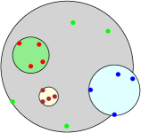
Figure 1: Quorum clustering for $n=16$ and $k=4$.

Given a set $\mathsf{P}$ of $n$ points in ${\rm I\!R}^{d}$, and a number $k\geq 1$, where $k|n$, we start with the smallest ball $\mathsf{b}_{1}$ that contains $k$ points of $\mathsf{P}$, that is $\mathrm{radius}({\mathsf{b}_{1}})=r_{\mathrm{opt}}\!\left({{\mathsf{P}},{k}}\right)$. Let $\mathsf{P}_{1}=\mathsf{P}\cap\mathsf{b}_{1}$. Continue on the set of points $\mathsf{P}\setminus\mathsf{P}_{1}$ by finding the smallest ball that contains $k$ points of $\mathsf{P}\setminus\mathsf{P}_{1}$, and so on. Let $\mathsf{b}_{1},\mathsf{b}_{2},\dots,\mathsf{b}_{n/k}$ denote the set of balls computed by this algorithm and let $\mathsf{P}_{i}=\!\left({\mathsf{P}\setminus\!\left({\mathsf{P}_{1}\cup\dots\cup\mathsf{P}_{i-1}}\right)}\right)\cap\mathsf{b}_{i}$. See Figure 1 for an example. Let $\mathsf{c}_{i}$ and $\mathsf{r}_{i}$ denote the center and radius respectively, of $\mathsf{b}_{i}$, for $i=1,\ldots,n/k$. A slight symbolic perturbation can guarantee that (i) each ball $\mathsf{b}_{i}$ contains exactly $k$ points of $\mathsf{P}$, and (ii) all the centers $\mathsf{c}_{1},\mathsf{c}_{2},\dots,\mathsf{c}_{k}$, are distinct points. Observe that $\mathsf{r}_{1}\leq\mathsf{r}_{2}\leq\dots\leq\mathsf{r}_{n/k}\leq\mathsf{diam}\!\left({{\mathsf{P}}}\right)$. Such a partition of $\mathsf{P}$ into $n/k$ clusters is a quorum clustering. An algorithm for computing it is provided in Carmi et al. [CDH⁺05]. We assume we have a black-box procedure QuorumCluster$(\mathsf{P},k)$ [CDH⁺05] that computes an approximate quorum clustering. It returns a list of balls, $(\mathsf{c}_{1},\mathsf{r}_{1}),\ldots,({\mathsf{c}_{n/k},\mathsf{r}_{n/k}})$. The algorithm of Carmi et al. [CDH⁺05] computes such a sequence of balls, where each ball is a $2$-approximation to the smallest ball containing $k$ points of the remaining points. The following is an improvement over the result of Carmi et al. [CDH⁺05].

Lemma 2.6.

Given a set $\mathsf{P}$ of $n$ points in ${\rm I\!R}^{d}$ and parameter $k$, where $k|n$, one can compute, in $O(n\log n)$ time, a sequence of $n/k$ balls, such that, for all $i,1\leq i\leq n/k$, we have

1. For every ball $\hskip 0.6pt\left({\mathsf{c}_{i},\mathsf{r}_{i}}\right)$ there is an associated subset $\mathsf{P}_{i}$ of $k$ points of $\mathsf{Q}_{i}=\mathsf{P}\setminus\left({\mathsf{P}_{i}\cup\ldots\cup\mathsf{P}_{i-1}}\right)$, that it covers.

2. The ball $\hskip 0.6pt\left({\mathsf{c}_{i},\mathsf{r}_{i}}\right)$ is a $2$-approximation to the smallest ball covering $k$ points in $\mathsf{Q}_{i}$; that is, $\mathsf{r}_{i}/2\leq r_{\mathrm{opt}}\!\left({{\mathsf{Q}_{i}},{k}}\right)\leq\mathsf{r}_{i}$.

Proof.

The guarantee of Carmi et al. is slightly worse – their algorithm running time is $O(n\log^{d}n)$. They use a dynamic data-structure for answering $O(n)$ queries, that report how many points are inside a query canonical square. Since they use orthogonal range trees this requires $O(\log^{d}n)$ time per query. Instead, one can use dynamic quadtrees. More formally, we store the points using linear ordering [Har11], using any balanced data-structure. A query to decide the number of points inside a canonical node corresponds to an interval query (i.e., reporting the number of elements that are inside a query interval), and can be performed in $O(\log n)$ time. Plugging this data-structure into the algorithm of Carmi et al. [CDH⁺05] gives the desired result.

3 A $(15,k)$-ANN in sublinear space

Lemma 3.1.

Let $\mathsf{P}$ be a set of $n$ points in ${\rm I\!R}^{d}$, $k\geq 1$ be a number such that $k|n$, $\hskip 0.6pt\left({\mathsf{c}_{1},\mathsf{r}_{1}}\right),\ldots$, $\!\left({\mathsf{c}_{n/k},\mathsf{r}_{n/k}}\right)$, be the list of balls returned by QuorumCluster$(\mathsf{P},k)$, and let $x=\min_{i=1,\dots,n/k}$ $\!\left({\left\lVert{{\mathtt{q}}-{\mathsf{c}_{i}}}\right\rVert+\mathsf{r}_{i}}\right)$. We have that $x/5\leq\mathsf{d}_{k}\!\left({\mathtt{q},\mathsf{P}}\right)\leq x$.

Proof.

For any $i=1,\ldots,n/k,$ we have $\mathsf{b}_{i}=\mathsf{ball}\!\left({\mathsf{c}_{i},\mathsf{r}_{i}}\right)\subseteq\mathsf{ball}\!\left({\mathtt{q},\left\lVert{{\mathtt{q}}-{\mathsf{c}_{i}}}\right\rVert+\mathsf{r}_{i}}\right)$. Since $\left\lvert{\mathsf{b}_{i}\cap\mathsf{P}}\right\rvert\geq k$, we have $\mathsf{d}_{k}\!\left({\mathtt{q},\mathsf{P}}\right)\leq\left\lVert{{\mathtt{q}}-{\mathsf{c}_{i}}}\right\rVert+\mathsf{r}_{i}$. As such, $\mathsf{d}_{k}\!\left({\mathtt{q},\mathsf{P}}\right)\leq x=\displaystyle\min_{i=1,\dots,n/k}\!\left({\left\lVert{{\mathtt{q}}-{\mathsf{c}_{i}}}\right\rVert+\mathsf{r}_{i}}\right)$.

For the other direction, let $i$ be the first index such that $\mathsf{ball}\!\left({\mathtt{q},\mathsf{d}_{k}\!\left({\mathtt{q},\mathsf{P}}\right)}\right)$ contains a point of $\mathsf{P}_{i}$, where $\mathsf{P}_{i}$ is the set of $k$ points of $\mathsf{P}$ assigned to $\mathsf{b}_{i}$. Then, we have

$$\mathsf{r}_{i}/2\leq r_{\mathrm{opt}}\!\left({{\mathsf{Q}_{i}},{k}}\right)\leq\mathsf{d}_{k}\!\left({\mathtt{q},\mathsf{P}}\right),$$

where $\mathsf{Q}_{i}=\mathsf{P}\setminus(\mathsf{P}_{1}\cup\dots\cup\mathsf{P}_{i-1})$, $\mathsf{r}_{i}$ is a $2$-approximation to $r_{\mathrm{opt}}\!\left({{\mathsf{Q}_{i}},{k}}\right)$, and the last inequality follows as $X=\mathsf{ball}\!\left({\mathtt{q},\mathsf{d}_{k}\!\left({\mathtt{q},\mathsf{P}}\right)}\right)\cap\mathsf{P}$ is a set of size $k$ and $X\subseteq\mathsf{Q}_{i}$. Then,

$$\left\lVert{{\mathtt{q}}-{\mathsf{c}_{i}}}\right\rVert-\mathsf{r}_{i}\leq\mathsf{d}\!\left({\mathtt{q},\mathsf{ball}\!\left({\mathsf{c}_{i},\mathsf{r}_{i}}\right)}\right)\leq\mathsf{d}_{k}\!\left({\mathtt{q},\mathsf{P}}\right),$$

as the distance from $\mathtt{q}$ to any $\mathsf{u}\in\mathsf{ball}\!\left({\mathsf{c}_{i},\mathsf{r}_{i}}\right)$ satisfies $\left\lVert{{\mathtt{q}}-{\mathsf{u}}}\right\rVert\geq\left\lVert{{\mathtt{q}}-{\mathsf{c}_{i}}}\right\rVert-\mathsf{r}_{i}$ by the triangle inequality. Putting the above together, we get

$$x=\min_{j=1,\dots,n/k}\!\left({\left\lVert{{\mathtt{q}}-{\mathsf{c}_{j}}}\right\rVert+\mathsf{r}_{j}}\right)\leq\left\lVert{{\mathtt{q}}-{\mathsf{c}_{i}}}\right\rVert+\mathsf{r}_{i}=\left({\left\lVert{{\mathtt{q}}-{\mathsf{c}_{i}}}\right\rVert-\mathsf{r}_{i}}\right)+2\mathsf{r}_{i}\leq 5\mathsf{d}_{k}\!\left({\mathtt{q},\mathsf{P}}\right).$$

Theorem 3.2.

Given a set $\mathsf{P}$ of $n$ points in ${\rm I\!R}^{d}$, and a number $k\geq 1$ such that $k|n$, one can build a data-structure, in $O\!\left({n\log n}\right)$ time, that uses $O\!\left({n/k}\right)$ space, such that given any query point $\mathtt{q}\in{\rm I\!R}^{d}$, one can compute, in $O\!\left({\log\!\left({n/k}\right)}\right)$ time, a $15$-approximation to $\mathsf{d}_{k}\!\left({\mathtt{q},\mathsf{P}}\right)$.

Proof.

We invoke QuorumCluster$(\mathsf{P},k)$ to compute the clusters $\left({\mathsf{c}_{i},\mathsf{r}_{i}}\right)$, for $i=1,\ldots,n/k$. For $i=1,\ldots,n/k$, let $\mathsf{b}_{i}^{\prime}=\!\left({\mathsf{c}_{i},\mathsf{r}_{i}}\right)\in{\rm I\!R}^{d+1}$. We preprocess the set $\mathcal{B}^{\prime}=\left\{{\mathsf{b}_{1}^{\prime},\ldots,\mathsf{b}_{n/k}^{\prime}}\right\}$ for $2$-ANN queries (in ${\rm I\!R}^{d+1}$ under the Euclidean norm). The preprocessing time for the ANN data structure is $O\!\left({\!\left({n/k}\right)\log\!\left({n/k}\right)}\right)$, the space used is $O\!\left({n/k}\right)$ and the query time is $O\!\left({\log\!\left({n/k}\right)}\right)$ [Har11].

Given a query point $\mathtt{q}\in{\rm I\!R}^{d}$ the algorithm computes a $2$-ANN to $\mathtt{q}^{\prime}=\left({\mathtt{q},0}\right)$, denoted by $\mathsf{b}_{j}^{\prime}$, and returns $\left\lVert{{\mathtt{q}^{\prime}}-{\mathsf{b}_{j}^{\prime}}}\right\rVert_{\oplus}$ as the approximate distance.

Observe that, for any $i$, we have $\left\lVert{{\mathtt{q}^{\prime}}-{\mathsf{b}_{i}^{\prime}}}\right\rVert\leq\left\lVert{{\mathtt{q}^{\prime}}-{\mathsf{b}_{i}^{\prime}}}\right\rVert_{\oplus}\leq\sqrt{2}\left\lVert{{\mathtt{q}^{\prime}}-{\mathsf{b}_{i}^{\prime}}}\right\rVert$ by Lemma 2.3. As such, the returned distance to $\mathsf{b}_{j}^{\prime}$ is a $2$-approximation to $\mathsf{d}\!\left({\mathtt{q}^{\prime},\mathcal{B}^{\prime}}\right)$; that is,

$${\mathsf{d}_{\oplus}\!\left({\mathtt{q}^{\prime},\mathcal{B}^{\prime}}\right)}\leq\left\lVert{{\mathtt{q}^{\prime}}-{\mathsf{b}_{j}^{\prime}}}\right\rVert_{\oplus}\leq\sqrt{2}\left\lVert{{\mathtt{q}^{\prime}}-{\mathsf{b}_{j}^{\prime}}}\right\rVert\leq 2\sqrt{2}\mathsf{d}\!\left({\mathtt{q}^{\prime},\mathcal{B}^{\prime}}\right)\leq 2\sqrt{2}\mathsf{d}_{\oplus}\!\left({\mathtt{q}^{\prime},\mathcal{B}^{\prime}}\right).$$

By Lemma 3.1, $\mathsf{d}_{\oplus}\!\left({\mathtt{q}^{\prime},\mathcal{B}^{\prime}}\right)/5\leq\mathsf{d}_{k}\!\left({\mathtt{q},\mathsf{P}}\right)\leq\mathsf{d}_{\oplus}\!\left({\mathtt{q}^{\prime},\mathcal{B}^{\prime}}\right)$. Namely,

$$\left\lVert{{\mathtt{q}^{\prime}}-{\mathsf{b}_{j}^{\prime}}}\right\rVert_{\oplus}/(10\sqrt{2})\leq\mathsf{d}_{k}\!\left({\mathtt{q},\mathsf{P}}\right)\leq\left\lVert{{\mathtt{q}^{\prime}}-{\mathsf{b}_{j}^{\prime}}}\right\rVert_{\oplus},$$

implying the claim.

Remark 3.3.

The algorithm of Theorem 3.2 works for any metric space. Given a set $\mathsf{P}$ of $n$ points in a metric space, one can compute $n/k$ points in the product space induced by adding an extra coordinate, such that approximating the distance to the $k$th nearest neighbor, is equivalent to answering ANN queries on the reduced point set, in the product space.

4 Approximate Voronoi diagram for $\mathsf{d}_{k}\!\left({\mathtt{q},\mathsf{P}}\right)$

Here, we are given a set $\mathsf{P}$ of $n$ points in ${\rm I\!R}^{d}$, and our purpose is to build an AVD that approximates the $k$-ANN distance, while using (roughly) $O(n/k)$ space.

4.1 Construction

4.1.1 Preprocessing

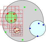
Figure 2: Quorum clustering, immediate environs and grids.

1. Compute a quorum clustering for $\mathsf{P}$ using Lemma 2.6. Let the list of balls returned be $\mathsf{b}_{1}=\!\left({\mathsf{c}_{1},\mathsf{r}_{1}}\right),\dots,\mathsf{b}_{n/k}=\!\left({\mathsf{c}_{n/k},\mathsf{r}_{n/k}}\right)$.

2. Compute an exponential grid around each quorum cluster. Specifically, let

   $$\displaystyle\mathcal{X}=\,\bigcup_{i=1}^{n/k}\;\;\bigcup_{j=0}^{\left\lceil{\log\left({32/{\varepsilon}}\right)+1}\right\rceil}\boxplus\!\left({\mathsf{ball}\!\left({\mathsf{c}_{i},2^{j}\mathsf{r}_{i}}\right),\frac{{\varepsilon}}{\zeta_{1}d}2^{j}\mathsf{r}_{i}}\right)$$ (1)

   be the set of grid cells covering the quorum clusters and their immediate environ, where $\zeta_{1}$ is a sufficiently large constant, see Figure 2.

3. Intuitively, $\mathcal{X}$ takes care of the region of space immediately next to a quorum cluster. For the other regions of space, we can apply a construction of an approximate Voronoi diagram for the centers of the clusters (the details are somewhat more involved). To this end, lift the quorum clusters into points in ${\rm I\!R}^{d+1}$, as follows

   $$\mathcal{B}^{\prime}=\left\{{\mathsf{b}_{1}^{\prime},\dots,\mathsf{b}_{n/k}^{\prime}}\right\},$$

   where $\mathsf{b}_{i}^{\prime}=\!\left({\mathsf{c}_{i},\mathsf{r}_{i}}\right)\in{\rm I\!R}^{d+1}$, for $i=1,\ldots,n/k$. Note, that all points in $\mathcal{B}^{\prime}$ belong to $U^{\prime}=[0,1]^{d+1}$ by Assumption 2.5. Now build a $(1+{\varepsilon}/8)$-AVD for $\mathcal{B}^{\prime}$ using the algorithm of Arya and Malamatos [AM02]. The AVD construction provides a list of canonical cubes covering $[0,1]^{d+1}$ such that in the smallest cube containing the query point, the associated point of $\mathcal{B}^{\prime}$, is a $(1+{\varepsilon}/8)$-ANN to the query point. (Note, that these cubes are not necessarily disjoint. In particular, the smallest cube containing the query point $\mathtt{q}$ is the one that determines the assigned approximate nearest neighbor to $\mathtt{q}$.)

   Clip this collection of cubes to the hyperplane $x_{d+1}=0$ (i.e., throw away cubes that do not have a face on this hyperplane). For a cube $\mathsf{\Box}$ in this collection, denote by $\mathrm{nn^{\prime}}\!\left({\mathsf{\Box}}\right)$, the point of $\mathcal{B}^{\prime}$ assigned to it. Let $\mathcal{S}$ be this resulting set of canonical $d$-dimensional cubes.

4. Let $\mathcal{W}$ be the space decomposition resulting from overlaying the two collection of cubes, i.e. $\mathcal{X}$ and $\mathcal{S}$. Formally, we compute a compressed quadtree $\mathcal{T}$ that has all the canonical cubes of $\mathcal{X}$ and $\mathcal{S}$ as nodes, and $\mathcal{W}$ is the resulting decomposition of space into cells. One can overlay two compressed quadtrees representing the two sets in linear time [dBHTT10, Har11]. Here, a cell associated with a leaf is a canonical cube, and a cell associated with a compressed node is the set difference of two canonical cubes. Each node in this compressed quadtree contains two pointers – to the smallest cube of $\mathcal{X}$, and to the smallest cube of $\mathcal{S}$, that contains it. This information can be computed by doing a BFS on the tree.

   For each cell $\mathsf{\Box}\in\mathcal{W}$ we store the following.

   1. An arbitrary representative point $\mathsf{\Box}_{\mathsf{rep}}\in\mathsf{\Box}$.

   2. The point $\mathrm{nn^{\prime}}\!\left({\mathsf{\Box}}\right)\in\mathcal{B}^{\prime}$ that is associated with the smallest cell of $\mathcal{S}$ that contains this cell. We also store an arbitrary point, $\mathbf{p}\!\left({\mathsf{\Box}}\right)\in\mathsf{P}$, that is one of the $k$ points belonging to the cluster specified by $\mathrm{nn^{\prime}}\!\left({\mathsf{\Box}}\right)$.

   3. A number $\mathrm{\beta}_{k}\!\left({\mathsf{\Box}_{\mathsf{rep}}}\right)$ that satisfies $\mathsf{d}_{k}\!\left({\mathsf{\Box}_{\mathsf{rep}},\mathsf{P}}\right)\leq\mathrm{\beta}_{k}\!\left({\mathsf{\Box}_{\mathsf{rep}}}\right)\leq(1+{\varepsilon}/4)\mathsf{d}_{k}\!\left({\mathsf{\Box}_{\mathsf{rep}},\mathsf{P}}\right)$, and a point $\mathrm{nn}_{k}\!\left({\mathsf{\Box}_{\mathsf{rep}}}\right)\in\mathsf{P}$ that realizes this distance. In order to compute $\mathrm{\beta}_{k}\!\left({\mathsf{\Box}_{\mathsf{rep}}}\right)$ and $\mathrm{nn}_{k}\!\left({\mathsf{\Box}_{\mathsf{rep}}}\right)$ use the data-structure of Section 6 (see Theorem 6.3) or the data-structure of Arya et al. [AMM05].

4.1.2 Answering a query

Given a query point $\mathtt{q}$, compute the leaf cell (equivalently the smallest cell) in $\mathcal{W}$ that contains $\mathtt{q}$ by performing a point-location query in the compressed quadtree $\mathcal{T}$. Let $\mathsf{\Box}$ be this cell. Return

$$\min\!\left({\rule[-5.69046pt]{0.0pt}{11.38092pt}\left\lVert{{\mathtt{q}^{\prime}}-{\mathrm{nn^{\prime}}\!\left({\mathsf{\Box}}\right)}}\right\rVert_{\oplus},\,\mathrm{\beta}_{k}\!\left({\mathsf{\Box}_{\mathsf{rep}}}\right)+\left\lVert{{\mathtt{q}}-{\mathsf{\Box}_{\mathsf{rep}}}}\right\rVert}\right),$$ (2)

as the approximate value to $\mathsf{d}_{k}\!\left({\mathtt{q},\mathsf{P}}\right)$. Return either $\mathbf{p}\!\left({\mathsf{\Box}}\right)$ or $\mathrm{nn}_{k}\!\left({\mathsf{\Box}_{\mathsf{rep}}}\right)$ depending on which of the two distances $\left\lVert{{\mathtt{q}^{\prime}}-{\mathrm{nn^{\prime}}\!\left({\mathsf{\Box}}\right)}}\right\rVert_{\oplus}$ or $\mathrm{\beta}_{k}\!\left({\mathsf{\Box}_{\mathsf{rep}}}\right)+\left\lVert{{\mathtt{q}}-{\mathsf{\Box}_{\mathsf{rep}}}}\right\rVert$ is smaller (this is the returned approximate value of $\mathsf{d}_{k}\!\left({\mathtt{q},\mathsf{P}}\right)$), as the approximate $k$th-nearest neighbor.

4.2 Correctness

Lemma 4.1.

Let $\mathsf{\Box}\in\mathcal{W}$ and $\mathtt{q}\in\mathsf{\Box}$. Then the number computed by the algorithm is an upper bound on $\mathsf{d}_{k}\!\left({\mathtt{q},\mathsf{P}}\right)$.

Proof.

By Observation 2.1, $\mathsf{d}_{k}\!\left({\mathtt{q},\mathsf{P}}\right)\leq\mathsf{d}_{k}\!\left({\mathsf{\Box}_{\mathsf{rep}},\mathsf{P}}\right)+\left\lVert{{\mathtt{q}}-{\mathsf{\Box}_{\mathsf{rep}}}}\right\rVert\leq\mathrm{\beta}_{k}\!\left({\mathsf{\Box}_{\mathsf{rep}}}\right)+\left\lVert{{\mathtt{q}}-{\mathsf{\Box}_{\mathsf{rep}}}}\right\rVert$. Now, let $\mathrm{nn^{\prime}}\!\left({\mathsf{\Box}}\right)=(\mathsf{c},\mathsf{r})$. We have, by Lemma 3.1, that $\mathsf{d}_{k}\!\left({\mathtt{q},\mathsf{P}}\right)\leq\left\lVert{{\mathtt{q}}-{\mathsf{c}}}\right\rVert+\mathsf{r}=\left\lVert{{\mathtt{q}^{\prime}}-{\mathrm{nn^{\prime}}\!\left({\mathsf{\Box}}\right)}}\right\rVert_{\oplus}.$ As the returned value is the minimum of these two numbers, the claim holds.

Lemma 4.2.

Consider any query point $\mathtt{q}\in[0,1]^{d}$, and let $\mathsf{\Box}$ be the smallest cell of $\mathcal{W}$ that contains the query point. Then, $\mathsf{d}\!\left({\mathtt{q}^{\prime},\mathcal{B}^{\prime}}\right)\leq\left\lVert{{\mathtt{q}^{\prime}}-{\mathrm{nn^{\prime}}\!\left({\mathsf{\Box}}\right)}}\right\rVert\leq(1+{\varepsilon}/8)\mathsf{d}\!\left({\mathtt{q}^{\prime},\mathcal{B}^{\prime}}\right)$.

Proof.

Observe that the space decomposition generated by $\mathcal{W}$ is a refinement of the decomposition generated by the Arya and Malamatos [AM02] AVD construction, when applied to $\mathcal{B}^{\prime}$, and restricted to the $d$ dimensional subspace we are interested in (i.e., $x_{d+1}=0$). As such, $\mathrm{nn^{\prime}}\!\left({\mathsf{\Box}}\right)$ is the point returned by the AVD for this query point before the refinement, thus implying the claim.

4.2.1 The query point is close to a quorum cluster of the right size

Lemma 4.3.

Consider a query point $\mathtt{q}$, and let $\mathsf{\Box}\subseteq{\rm I\!R}^{d}$ be any set with $\mathtt{q}\in\mathsf{\Box}$, such that $\mathsf{diam}\!\left({{\mathsf{\Box}}}\right)\leq{\varepsilon}\mathsf{d}_{k}\!\left({\mathtt{q},\mathsf{P}}\right)$. Then, for any $\mathsf{u}\in\mathsf{\Box}$, we have

$$(1-{\varepsilon})\mathsf{d}_{k}\!\left({\mathtt{q},\mathsf{P}}\right)\leq\mathsf{d}_{k}\!\left({\mathsf{u},\mathsf{P}}\right)\leq(1+{\varepsilon})\mathsf{d}_{k}\!\left({\mathtt{q},\mathsf{P}}\right).$$

Proof.

By Observation 2.1, we have

$$\mathsf{d}_{k}\!\left({\mathtt{q},\mathsf{P}}\right)\leq\mathsf{d}_{k}\!\left({\mathsf{u},\mathsf{P}}\right)+\left\lVert{{\mathsf{u}}-{\mathtt{q}}}\right\rVert\leq\mathsf{d}_{k}\!\left({\mathsf{u},\mathsf{P}}\right)+\mathsf{diam}\!\left({{\mathsf{\Box}}}\right)\leq\mathsf{d}_{k}\!\left({\mathsf{u},\mathsf{P}}\right)+{\varepsilon}\mathsf{d}_{k}\!\left({\mathtt{q},\mathsf{P}}\right).$$

The other direction follows by a symmetric argument.

Lemma 4.4.

If the smallest region $\mathsf{\Box}\in\mathcal{W}$ that contains $\mathtt{q}$ has diameter $\mathsf{diam}\!\left({{\mathsf{\Box}}}\right)\leq{\varepsilon}\mathsf{d}_{k}\!\left({\mathtt{q},\mathsf{P}}\right)/4$, then the algorithm returns a distance which is between $\mathsf{d}_{k}\!\left({\mathtt{q},\mathsf{P}}\right)$ and $(1+{\varepsilon})\mathsf{d}_{k}\!\left({\mathtt{q},\mathsf{P}}\right)$.

Proof.

Let $\mathsf{\Box}_{\mathsf{rep}}$ be the representative stored with the cell. Let $\alpha$ be the number returned by the algorithm. By Lemma 4.1 we have that $\mathsf{d}_{k}\!\left({\mathtt{q},\mathsf{P}}\right)\leq\alpha$. Since the algorithm returns the minimum of two numbers, one of which is $\mathrm{\beta}_{k}\!\left({\mathsf{\Box}_{\mathsf{rep}}}\right)+\left\lVert{{\mathtt{q}}-{\mathsf{\Box}_{\mathsf{rep}}}}\right\rVert$, we have by Lemma 4.3,

$$\alpha\; \leq\mathrm{\beta}_{k}\!\left({\mathsf{\Box}_{\mathsf{rep}}}\right)+\left\lVert{{\mathtt{q}}-{\mathsf{\Box}_{\mathsf{rep}}}}\right\rVert\leq(1+{\varepsilon}/4)\mathsf{d}_{k}\!\left({\mathsf{\Box}_{\mathsf{rep}},\mathsf{P}}\right)+\left\lVert{{\mathtt{q}}-{\mathsf{\Box}_{\mathsf{rep}}}}\right\rVert$$

$$\leq(1+{\varepsilon}/4)\!\left({\rule[-5.69046pt]{0.0pt}{11.38092pt}\mathsf{d}_{k}\!\left({\mathtt{q},\mathsf{P}}\right)+\mathsf{diam}\!\left({{\mathsf{\Box}}}\right)}\right)+\mathsf{diam}\!\left({{\mathsf{\Box}}}\right)$$

$$\leq(1+{\varepsilon}/4)(\mathsf{d}_{k}\!\left({\mathtt{q},\mathsf{P}}\right)+{\varepsilon}\mathsf{d}_{k}\!\left({\mathtt{q},\mathsf{P}}\right)/4)+{\varepsilon}\mathsf{d}_{k}\!\left({\mathtt{q},\mathsf{P}}\right)/4$$

$$=(1+{\varepsilon}/4)^{2}\mathsf{d}_{k}\!\left({\mathtt{q},\mathsf{P}}\right)+{\varepsilon}\mathsf{d}_{k}\!\left({\mathtt{q},\mathsf{P}}\right)/4\leq(1+{\varepsilon})\mathsf{d}_{k}\!\left({\mathtt{q},\mathsf{P}}\right),$$

establishing the claim.

Definition 4.5.

Consider a query point $\mathtt{q}\in{\rm I\!R}^{d}$. The first quorum cluster $\mathsf{b}_{i}=\mathsf{ball}\!\left({\mathsf{c}_{i},\mathsf{r}_{i}}\right)$ that intersects $\mathsf{ball}\!\left({\mathtt{q},\mathsf{d}_{k}\!\left({\mathtt{q},\mathsf{P}}\right)}\right)$ is the anchor cluster of $\mathtt{q}$. The corresponding anchor point is $\left({\mathsf{c}_{i},\mathsf{r}_{i}}\right)\in{\rm I\!R}^{d+1}$.

Lemma 4.6.

For any query point $\mathtt{q}$, we have that

1. the anchor point $\!\left({\mathsf{c},\mathsf{r}}\right)$ is well defined,

2. $\mathsf{r}\leq 2\mathsf{d}_{k}\!\left({\mathtt{q},\mathsf{P}}\right)$,

3. for $\mathsf{b}=\mathsf{ball}\!\left({\mathsf{c},\mathsf{r}}\right)$ we have $\mathsf{b}\cap\mathsf{ball}\!\left({\mathtt{q},\mathsf{d}_{k}\!\left({\mathtt{q},\mathsf{P}}\right)}\right)\neq\emptyset$, and

4. $\left\lVert{{\mathtt{q}}-{\mathsf{c}}}\right\rVert\leq 3\mathsf{d}_{k}\!\left({\mathtt{q},\mathsf{P}}\right)$.

Proof.

Consider the $k$ closest points to $\mathtt{q}$ in $\mathsf{P}$. As $\mathsf{P}\subseteq\mathsf{b}_{1}\cup\dots\cup\mathsf{b}_{n/k}$ it must be that $\mathsf{ball}\!\left({\mathtt{q},\mathsf{d}_{k}\!\left({\mathtt{q},\mathsf{P}}\right)}\right)$ intersects some $\mathsf{b}_{i}$. Consider the first cluster $\mathsf{ball}\!\left({\mathsf{c},\mathsf{r}}\right)$ in the quorum clustering that intersects $\mathsf{ball}\!\left({\mathtt{q},\mathsf{d}_{k}\!\left({\mathtt{q},\mathsf{P}}\right)}\right)$. Then $\!\left({\mathsf{c},\mathsf{r}}\right)$ is by definition the anchor point and we immediately have $\mathsf{ball}\!\left({\mathsf{c},\mathsf{r}}\right)\cap\mathsf{ball}\!\left({\mathtt{q},\mathsf{d}_{k}\!\left({\mathtt{q},\mathsf{P}}\right)}\right)\neq\emptyset$. Claim (ii) is implied by the proof of Lemma 3.1. Finally, as for (iv), we have $\mathsf{r}\leq 2\mathsf{d}_{k}\!\left({\mathtt{q},\mathsf{P}}\right)$ and the ball around $\mathtt{q}$ of radius $\mathsf{d}_{k}\!\left({\mathtt{q},\mathsf{P}}\right)$ intersects $\mathsf{ball}\!\left({\mathsf{c},\mathsf{r}}\right)$, thus implying that $\left\lVert{{\mathtt{q}}-{\mathsf{c}}}\right\rVert\leq\mathsf{d}_{k}\!\left({\mathtt{q},\mathsf{P}}\right)+\mathsf{r}\leq 3\mathsf{d}_{k}\!\left({\mathtt{q},\mathsf{P}}\right)$.

Lemma 4.7.

Consider a query point $\mathtt{q}$. If there is a cluster $\mathsf{ball}\!\left({\mathsf{c},\mathsf{r}}\right)$ in the quorum clustering computed, such that $\left\lVert{{\mathtt{q}}-{\mathsf{c}}}\right\rVert\leq 6\mathsf{d}_{k}\!\left({\mathtt{q},\mathsf{P}}\right)$ and ${\varepsilon}\mathsf{d}_{k}\!\left({\mathtt{q},\mathsf{P}}\right)/4\leq\mathsf{r}\leq 6\mathsf{d}_{k}\!\left({\mathtt{q},\mathsf{P}}\right)$, then the output of the algorithm is correct.

Proof.

We have

$$\frac{32\mathsf{r}}{{\varepsilon}}\geq\frac{32({\varepsilon}\mathsf{d}_{k}\!\left({\mathtt{q},\mathsf{P}}\right)/4)}{{\varepsilon}}=8\mathsf{d}_{k}\!\left({\mathtt{q},\mathsf{P}}\right)\geq\left\lVert{{\mathtt{q}}-{\mathsf{c}}}\right\rVert.$$

Thus, by construction, the expanded environ of the quorum cluster $\mathsf{ball}\!\left({\mathsf{c},\mathsf{r}}\right)$ contains the query point, see Eq. (1)${}_{\text{p\ref{equation:clusters:around:q}}}$. Let $j$ be the smallest integer such that $2^{j}\mathsf{r}\geq\left\lVert{{\mathtt{q}}-{\mathsf{c}}}\right\rVert$. We have that, $2^{j}\mathsf{r}\leq\max(\mathsf{r},2\left\lVert{{\mathtt{q}}-{\mathsf{c}}}\right\rVert)$. As such, if $\mathsf{\Box}$ is the smallest cell in $\mathcal{W}$ containing the query point $\mathtt{q}$, then

$$\mathsf{diam}\!\left({{\mathsf{\Box}}}\right) \leq\frac{{\varepsilon}}{\zeta_{1}d}2^{j}\mathsf{r}\leq\frac{{\varepsilon}}{\zeta_{1}d}\cdot\max\!\left({\mathsf{r},2\left\lVert{{\mathtt{q}}-{\mathsf{c}}}\right\rVert}\right)\leq\frac{{\varepsilon}}{\zeta_{1}d}\cdot\max\!\left({6\mathsf{d}_{k}\!\left({\mathtt{q},\mathsf{P}}\right),12\mathsf{d}_{k}\!\left({\mathtt{q},\mathsf{P}}\right)\rule[-5.69046pt]{0.0pt}{11.38092pt}}\right)$$

$$\leq\frac{{\varepsilon}}{4d}\mathsf{d}_{k}\!\left({\mathtt{q},\mathsf{P}}\right),$$

by Eq. (1)${}_{\text{p\ref{equation:clusters:around:q}}}$ and if $\zeta_{1}\geq 48$. As such, $\mathsf{diam}\!\left({{\mathsf{\Box}}}\right)\leq{\varepsilon}\mathsf{d}_{k}\!\left({\mathtt{q},\mathsf{P}}\right)/4$, and the claim follows by Lemma 4.3.

4.2.2 The general case

Lemma 4.8.

The data-structure constructed above returns $(1+{\varepsilon})$-approximation to $\mathsf{d}_{k}\!\left({\mathtt{q},\mathsf{P}}\right)$, for any query point $\mathtt{q}$.

Proof.

Consider the query point $\mathtt{q}$ and its anchor point $(\mathsf{c},\mathsf{r})$. By Lemma 4.6, we have $\mathsf{r}\leq 2\mathsf{d}_{k}\!\left({\mathtt{q},\mathsf{P}}\right)$ and $\left\lVert{{\mathtt{q}}-{\mathsf{c}}}\right\rVert\leq 3\mathsf{d}_{k}\!\left({\mathtt{q},\mathsf{P}}\right)$. This implies that

$$\mathsf{d}\!\left({\mathtt{q}^{\prime},\mathcal{B}^{\prime}}\right)\leq\left\lVert{{\mathtt{q}^{\prime}}-{(\mathsf{c},\mathsf{r})}}\right\rVert\leq\left\lVert{{\mathtt{q}}-{\mathsf{c}}}\right\rVert+\mathsf{r}\leq 5\mathsf{d}_{k}\!\left({\mathtt{q},\mathsf{P}}\right).$$ (3)

Let the returned point, which is a $(1+{\varepsilon}/8)$-ANN for $\mathtt{q}^{\prime}$ in $\mathcal{B}^{\prime}$, be $(\mathsf{c}_{\mathtt{q}},\mathsf{r}_{\mathtt{q}})=\mathrm{nn^{\prime}}\!\left({\mathsf{\Box}}\right)$, where $\mathtt{q}^{\prime}=\left({\mathtt{q},0}\right)$. We have that $\left\lVert{{\mathtt{q}^{\prime}}-{(\mathsf{c}_{\mathtt{q}},\mathsf{r}_{\mathtt{q}})}}\right\rVert\leq(1+{\varepsilon}/8)\mathsf{d}\!\left({\mathtt{q}^{\prime},\mathcal{B}^{\prime}}\right)\leq 6\mathsf{d}_{k}\!\left({\mathtt{q},\mathsf{P}}\right)$. In particular, $\left\lVert{{\mathtt{q}}-{\mathsf{c}_{\mathtt{q}}}}\right\rVert\leq 6\mathsf{d}_{k}\!\left({\mathtt{q},\mathsf{P}}\right)$ and $\mathsf{r}_{\mathtt{q}}\leq 6\mathsf{d}_{k}\!\left({\mathtt{q},\mathsf{P}}\right)$.

Thus, if $\mathsf{r}_{\mathtt{q}}\geq{\varepsilon}\mathsf{d}_{k}\!\left({\mathtt{q},\mathsf{P}}\right)/4$ or $\mathsf{r}\geq{\varepsilon}\mathsf{d}_{k}\!\left({\mathtt{q},\mathsf{P}}\right)/4$ we are done, by Lemma 4.7. Otherwise, we have

$$\left\lVert{{\mathtt{q}^{\prime}}-{\!\left({\mathsf{c}_{\mathtt{q}},\mathsf{r}_{\mathtt{q}}}\right)}}\right\rVert\leq(1+{\varepsilon}/8)\left\lVert{{\mathtt{q}^{\prime}}-{\!\left({\mathsf{c},\mathsf{r}}\right)}}\right\rVert,$$

as $\!\left({\mathsf{c}_{\mathtt{q}},\mathsf{r}_{\mathtt{q}}}\right)$ is a $(1+{\varepsilon}/8)$ approximation to $\mathsf{d}\!\left({\mathtt{q}^{\prime},\mathcal{B}^{\prime}}\right)$. As such,

$$\frac{\left\lVert{{\mathtt{q}^{\prime}}-{\!\left({\mathsf{c}_{\mathtt{q}},\mathsf{r}_{\mathtt{q}}}\right)}}\right\rVert}{1+{\varepsilon}/8}\leq\left\lVert{{\mathtt{q}^{\prime}}-{\!\left({\mathsf{c},\mathsf{r}}\right)}}\right\rVert\leq\left\lVert{{\mathtt{q}}-{\mathsf{c}}}\right\rVert+\mathsf{r}.$$ (4)

As $\mathsf{ball}\!\left({\mathsf{c},\mathsf{r}}\right)\cap\mathsf{ball}\!\left({\mathtt{q},\mathsf{d}_{k}\!\left({\mathtt{q},\mathsf{P}}\right)}\right)\neq\emptyset$ we have, by the triangle inequality, that

$$\left\lVert{{\mathtt{q}}-{\mathsf{c}}}\right\rVert-\mathsf{r}\leq\mathsf{d}_{k}\!\left({\mathtt{q},\mathsf{P}}\right).$$ (5)

By Eq. (4) and Eq. (5) we have

$$\frac{\left\lVert{{\mathtt{q}^{\prime}}-{\!\left({\mathsf{c}_{\mathtt{q}},\mathsf{r}_{\mathtt{q}}}\right)}}\right\rVert}{1+{\varepsilon}/8}-2\mathsf{r}\leq\left\lVert{{\mathtt{q}}-{\mathsf{c}}}\right\rVert-\mathsf{r}\leq\mathsf{d}_{k}\!\left({\mathtt{q},\mathsf{P}}\right).$$

By the above and as $\max\!\left({\mathsf{r},\mathsf{r}_{\mathtt{q}}}\right)<{\varepsilon}\mathsf{d}_{k}\!\left({\mathtt{q},\mathsf{P}}\right)/4$, we have

$$\left\lVert{{\mathtt{q}}-{\mathsf{c}_{\mathtt{q}}}}\right\rVert+\mathsf{r}_{\mathtt{q}} \leq\left\lVert{{\mathtt{q}^{\prime}}-{\!\left({\mathsf{c}_{\mathtt{q}},\mathsf{r}_{\mathtt{q}}}\right)}}\right\rVert+\mathsf{r}_{\mathtt{q}}\leq(1+{\varepsilon}/8)\!\left({\mathsf{d}_{k}\!\left({\mathtt{q},\mathsf{P}}\right)+2\mathsf{r}}\right)+\mathsf{r}_{\mathtt{q}}$$

$$\leq(1+{\varepsilon}/8)\!\left({\mathsf{d}_{k}\!\left({\mathtt{q},\mathsf{P}}\right)+{\varepsilon}\mathsf{d}_{k}\!\left({\mathtt{q},\mathsf{P}}\right)/2}\right)+{\varepsilon}\mathsf{d}_{k}\!\left({\mathtt{q},\mathsf{P}}\right)/4\leq(1+{\varepsilon})\mathsf{d}_{k}\!\left({\mathtt{q},\mathsf{P}}\right).$$

Since the algorithm returns for $\mathtt{q}$ a value that is at most $\left\lVert{{\mathtt{q}}-{\mathsf{c}_{\mathtt{q}}}}\right\rVert+\mathsf{r}_{\mathtt{q}}$, the result is correct.

4.3 The result

Theorem 4.9.

Given a set $\mathsf{P}$ of $n$ points in ${\rm I\!R}^{d}$, a number $k\geq 1$ such that $k|n$, and $0<{\varepsilon}$ sufficiently small, one can preprocess $\mathsf{P}$, in $\displaystyle O\!\left({n\log n+\frac{n}{k}C_{\varepsilon}\log n+\frac{n}{k}C_{\varepsilon}^{\prime}}\right)$ time, where $C_{\varepsilon}=O\!\left({{\varepsilon}^{-d}\log{{\varepsilon}}^{-1}}\right)$ and $C_{\varepsilon}^{\prime}=O\!\left({{\varepsilon}^{-2d+1}\log{{\varepsilon}}^{-1}}\right)$. The space used by the data-structure is $O(C_{\varepsilon}n/k)$. This data structure answers a $(1+{\varepsilon},k)$-ANN query in $\displaystyle O\!\left({\log\frac{n}{k{\varepsilon}}}\right)$ time. The data-structure also returns a point of $\mathsf{P}$ that is approximately the desired $k$-nearest neighbor.

Proof.

Computing the quorum clustering takes time $O\!\left({n\log n}\right)$ by Lemma 2.6. Observe that $\left\lvert{\mathcal{X}}\right\rvert=O\!\left({\frac{n}{k{\varepsilon}^{d}}\log\frac{1}{{\varepsilon}}}\right)$. From the construction of Arya and Malamatos [AM02], we have $\left\lvert{\mathcal{S}}\right\rvert=O\!\left({\frac{n}{k{\varepsilon}^{d}}\log\frac{1}{{\varepsilon}}}\right)$ (note, that since we clip the construction to a hyperplane, we get $1/{\varepsilon}^{d}$ in the bound and not $1/{\varepsilon}^{d+1}$). A careful implementation of this stage takes time $O\!\left({n\log n+\left\lvert{\mathcal{W}}\right\rvert\!\left({\log n+\frac{1}{{\varepsilon}^{d-1}}}\right)}\right)$. Overlaying the two compressed quadtrees representing them takes linear time in their size, that is $O\!\left({\left\lvert{\mathcal{X}}\right\rvert+\left\lvert{\mathcal{S}}\right\rvert}\right)$.

The most expensive step is to perform the $(1+{\varepsilon}/4,k)$-ANN query for each cell in the resulting decomposition of $\mathcal{W}$, see Eq. (2)${}_{\text{p\ref{equation:in:cell}}}$ (i.e., computing $\mathrm{\beta}_{k}\!\left({\mathsf{\Box}_{\mathsf{rep}}}\right)$ for each cell $\mathsf{\Box}\in\mathcal{W}$). Using the data-structure of Section 6 (see Theorem 6.3) each query takes $O\!\left({\log n+1/{\varepsilon}^{d-1}}\right)$ time (alternatively, we could use the data-structure of Arya et al. [AMM05]), As such, this takes

$$O\!\left({n\log n+\left\lvert{\mathcal{W}}\right\rvert\!\left({\log n+\frac{1}{{\varepsilon}^{d-1}}}\right)}\right)=O\!\left({n\log n+\frac{n}{k{\varepsilon}^{d}}\log\frac{1}{{\varepsilon}}\log n+\frac{n}{k{\varepsilon}^{2d-1}}\log\frac{1}{{\varepsilon}}}\right)$$

time, and this bounds the overall construction time.

The query algorithm is a point location query followed by an $O(1)$ time computation and takes time $O\!\left({\log\!\left({\frac{n}{k{\varepsilon}}}\right)}\right)$.

Finally, one needs to argue that the returned point of $\mathsf{P}$ is indeed the desired approximate $k$-nearest neighbor. This follows by arguing in a similar fashion to the correctness proof; the distance to the returned point is a $(1+{\varepsilon})$- approximation to the $k$th-nearest neighbor distance. We omit the tedious but straightforward details.

4.3.1 Using a single point for each AVD cell

The AVD generated can be viewed as storing two points in each cell $\mathsf{\Box}$ of the AVD. These two points are in ${\rm I\!R}^{d+1}$, and for a cell $\mathsf{\Box}$, they are

1. the point $\mathrm{nn^{\prime}}\!\left({\mathsf{\Box}}\right)\in\mathcal{B}^{\prime}$, and

2. the point $\!\left({\mathsf{\Box}_{\mathsf{rep}},\mathrm{\beta}_{k}\!\left({\mathsf{\Box}_{\mathsf{rep}}}\right)}\right)$.

The algorithm for $\mathsf{d}_{k}\!\left({\mathtt{q},\mathsf{P}}\right)$ can be viewed as computing the nearest neighbor of $\!\left({\mathtt{q},0}\right)$ to one of the above two points using the $\left\lVert{\cdot}\right\rVert_{\oplus}$ norm to define the distance. Using standard AVD algorithms we can subdivide each such cell $\mathsf{\Box}$ into $O\!\left({1/{\varepsilon}^{d}\log{\varepsilon}^{-1}}\right)$ cells to answer this query approximately. By using this finer subdivision we can have a single point inside each cell for which the closest distance is the approximation to $\mathsf{d}_{k}\!\left({\mathtt{q},\mathsf{P}}\right)$. This incurs an increase by a factor of $O\!\left({1/{\varepsilon}^{d}\log{\varepsilon}^{-1}}\right)$ in the number of cells.

4.4 A generalization – weighted version of $k$ ANN

We consider a generalization of the $(1+{\varepsilon},k)$-ANN problem. Specifically, we are given a set of points $\mathsf{P}\subseteq{\rm I\!R}^{d}$, a weight $w_{\mathsf{p}}\geq 0$ for each $\mathsf{p}\in\mathsf{P}$, and a number ${\varepsilon}>0$. Given a query $\mathtt{q}$ and weight $\tau\geq 0$, its $\tau$-NN distance to $\mathsf{P}$, is the minimum $r$ such that the closed ball $\mathsf{ball}\!\left({\mathtt{q},r}\right)$ contains points of $\mathsf{P}$ of total weight at least $\tau$. Formally, the $\tau$-NN distance for $\mathtt{q}$ is

$$\mathsf{d}_{\tau}\!\left({\mathtt{q},\mathsf{P}}\right)=\min\left\{{r\,\left|\,{w\!\left({\rule[-5.69046pt]{0.0pt}{11.38092pt}\mathsf{ball}\!\left({\mathtt{q},r}\right)\cap\mathsf{P}}\right)\geq\tau}\rule[-5.69046pt]{0.0pt}{11.38092pt}\right.}\right\},$$

where $w\!\left({X}\right)=\sum_{x\in X}w_{x}$. A $(1+{\varepsilon})$-approximate $\tau$-NN distance is a distance $\ell$, such that $(1-{\varepsilon})\mathsf{d}_{\tau}\!\left({\mathtt{q},\mathsf{P}}\right)\leq\ell\leq(1+{\varepsilon})\mathsf{d}_{\tau}\!\left({\mathtt{q},\mathsf{P}}\right)$ and a $(1+{\varepsilon})$-approximate $\tau$-NN is a point of $\mathsf{P}$ that realizes such a distance. The $(1+{\varepsilon},\tau)$-ANN problem is to preprocess $\mathsf{P}$, such that a $(1+{\varepsilon})$-approximate $\tau$-NN can be computed efficiently for any query point $\mathtt{q}$.

The $(1+{\varepsilon},k)$-ANN problem is the special case $w_{\mathsf{p}}=1$ for all $\mathsf{p}\in\mathsf{P}$ and $\tau=k$. Clearly, the function $\mathsf{d}_{\tau}\!\left({\cdot,\mathsf{P}}\right)$ is also a $1$-Lipschitz function of its argument. If we are given $\tau$ at the time of preprocessing, it can be verified that the $1$-Lipschitz property is enough to guarantee correctness of the AVD construction for the $(1+{\varepsilon},k)$-ANN problem. However, we need to compute a $\tau$ quorum clustering, where now each quorum cluster has weight at least $\tau$. A slight modification of the algorithm in Lemma 2.6 allows this. Moreover, for the preprocessing step which requires us to solve the $(1+{\varepsilon},\tau)$-ANN problem for the representative points, one can use the algorithm of Section 6.3. We get the following result,

Theorem 4.10.

Given a set of $n$ weighted points $\mathsf{P}$ in ${\rm I\!R}^{d}$, a number $\tau>0$ and $0<{\varepsilon}$ sufficiently small, one can preprocess $\mathsf{P}$ in $\displaystyle O\!\left({n\log n+\frac{w\!\left({\mathsf{P}}\right)}{\tau}C_{\varepsilon}\log n+\frac{w\!\left({\mathsf{P}}\right)}{\tau}C_{\varepsilon}^{\prime}}\right)$ time, where $C_{\varepsilon}=O\!\left({{\varepsilon}^{-d}\log{{\varepsilon}}^{-1}}\right)$ and $C_{\varepsilon}^{\prime}=O\!\left({{\varepsilon}^{-2d+1}\log{{\varepsilon}}^{-1}}\right)$ and $w\!\left({\mathsf{P}}\right)=\sum_{\mathsf{p}\in\mathsf{P}}w_{(}\mathsf{p})$. The space used by the data-structure is $O(C_{\varepsilon}w\!\left({\mathsf{P}}\right)/\tau)$. This data structure answers a $(1+{\varepsilon},\tau)$-ANN query in $\displaystyle O\!\left({\log\frac{w\!\left({\mathsf{P}}\right)}{\tau{\varepsilon}}}\right)$ time. The data-structure also returns a point of $\mathsf{P}$ that is a $(1+{\varepsilon})$-approximation to the $\tau$-nearest neighbor of the query point.

5 Density estimation

Given a point set $\mathsf{P}\subseteq{\rm I\!R}^{d}$, and a query point $\mathtt{q}\in{\rm I\!R}^{d}$, consider the point $\mathsf{v}(\mathtt{q})=(\mathsf{d}_{1}\!\left({\mathtt{q},\mathsf{P}}\right),\dots,$ $\mathsf{d}_{n}\!\left({\mathtt{q},\mathsf{P}}\right))$. This is a point in ${\rm I\!R}^{n}$, and several problems in Computational Geometry can be viewed as computing some interesting function of $\mathsf{v}(\mathtt{q})$. For example, one could view the nearest neighbor distance as the function that returns the first coordinate of $\mathsf{v}(\mathtt{q})$. Another motivating example is a geometric version of discrete density measures from Guibas et al. [GMM11]. In their problem one is interested in computing $g_{k}(\mathtt{q})=\sum_{i=1}^{k}\mathsf{d}_{i}\!\left({\mathtt{q},\mathsf{P}}\right)$. In this section, we show that a broad class of functions (that include $g_{k}$), can be approximated to within $(1\pm{\varepsilon})$, by a data structure requiring space $\widetilde{O}(n/k)$.

5.1 Performing point-location in several quadtrees simultaneously

Lemma 5.1.

Consider a rooted tree $T$ with $m$ nodes, where the nodes are colored by $I$ colors (a node might have several colors). Assume that there are $O(m)$ pairs of such $(\text{node},\text{color})$ associations. One can preprocess the tree in $O(m)$ time and space, such that given a query leaf $v$ of $T$, one can report the nodes $v_{1},\ldots,v_{I}$ in $O(I)$ time. Here, $v_{i}$ is the lowest node in the tree along the path from the root to $v$ that is colored with color $i$.

Proof.

We start with the naive solution – perform a DFS on $T$, and keep an array $\mathcal{X}$ of $I$ entries storing the latest node of each color encountered so far along the path from the root to the current node. Storing a snapshot of this array $\mathcal{X}$ at each node would require $O(mI)$ space. But then one can answer a query in $O(I)$ time. As such, the challenge is to reduce the required space.

To this end, interpret the DFS to be a Eulerian traversal of the tree. The traversal has length $2m-2$, and every edge traveled contains updates to the array $\mathcal{X}$. Indeed, if the DFS traverses down from a node $u$ to a child node $w$, the updates would be updating all the colors that are stored in $w$, to indicate that $w$ is the lowest node for these colors. Similarly, if the DFS goes up from $w$ to $u$, we restore all the colors stored in $w$ to their value just before the DFS visited $w$. Now, the DFS traversal of $T$ becomes a list of $O(m)$ updates. Each update is still an $O(I)$ operation. This is however a technicality, and can be resolved as follows. For each edge traveled we store the updates for all colors separately, each update being for a single color. Also each update entry stores the current node, i.e. the destination of the edge traveled. The total length of the update list is still $O(m)$, as follows from a simple charging argument, and the assumption about the number of $(\text{node},\text{color})$ pairs. We simply charge each restore to its corresponding “forward going” update, and the number of forward going updates is exactly equal to the number of $(\text{node},\text{color})$ pairs. For each leaf we store its last location in this list of updates.

So, let $L$ be this list of updates. At each $k$th update, for $k=tI$ for some integer $t$, store a snapshot of the array of colors as updated if we scan the list from the beginning till this point. Along with this we store the node at this point and auxiliary information allowing us to compute the next update i.e. if the snapshot stored is between all updates at this node. Clearly, all these snapshots can be computed in $O(m)$ time, and require $O((m/I)I)=O(m)$ space.

Now, given a query leaf $v$, we go to its location in the list $L$, and jump back to the last snapshot stored. We copy this snapshot, and then scan the list from the snapshot till the location for $v$. This would require re-doing at most $O(I)$ updates, and can be done in $O(I)$ time overall.

Lemma 5.2.

Given $I$ compressed quadtrees $\mathcal{D}_{1},\ldots,\mathcal{D}_{I}$ of total size $m$ in ${\rm I\!R}^{d}$, one can preprocess them in $O(m\log I)$ time, using $O(m)$ space, such that given a query point $\mathtt{q}$, one can perform point-location queries in all $I$ quadtrees, simultaneously for $\mathtt{q}$, in $O(\log m+I)$ time.

Proof.

Overlay all these compressed quadtrees together. Overlaying $I$ quadtrees is equivalent to merging $I$ sorted lists [Har11] and can be done in $O\!\left({m\log I}\right)$ time. Let $\mathcal{D}$ denote the resulting compressed quadtree. Note that any node of $\mathcal{D}_{i}$, for $i=1,\ldots,I$, must be a node in $\mathcal{D}$.

Given a query point $\mathtt{q}$, we need to extract the $I$ nodes in the original quadtrees $\mathcal{D}_{i}$, for $i=1,\ldots,I$, that contain the query point (these nodes can be compressed nodes). So, let $\mathsf{\Box}$ be the leaf node of $\mathcal{D}$ containing the query point $\mathtt{q}$. Consider the path $\pi$ from the root to the node $\mathsf{\Box}$. We are interested in the lowest node of $\pi$ that belongs to $\mathcal{D}_{i}$, for $i=1,\ldots,I$. To this end, color all the nodes of $\mathcal{D}_{i}$ that appear in $\mathcal{D}$, by color $i$, for $i=1,\ldots,I$. Now, we build the data-structure of Lemma 5.1 for $\mathcal{D}$. We can use this data-structure to answer the desired query in $O(I)$ time.

5.2 Slowly growing functions

$\mathcal{F}_{\mathsf{sg}}\rule[-5.69046pt]{0.0pt}{17.64056pt}$ The class of slowly growing functions, see Definition 5.3. $f\rule[-5.69046pt]{0.0pt}{17.64056pt}$ A function in $\mathcal{F}_{\mathsf{sg}}$ or a monotonic increasing function from ${\rm I\!R}$ to ${\rm I\!R}^{+}$. $F(\mathtt{q})$ $\sum_{i=1}^{k}f\!\left({\rule[0.0pt]{0.0pt}{9.95863pt}\mathsf{d}_{i}\!\left({\mathtt{q},\mathsf{P}}\right)}\right)$ ${F}_{1}(\mathtt{q})\rule[-5.69046pt]{0.0pt}{17.64056pt}$ $\sum_{i=\left\lceil{k{\varepsilon}/8}\right\rceil}^{k}f\!\left({\mathsf{d}_{i}\!\left({\mathtt{q},\mathsf{P}}\right)}\right)$ $\mathcal{I}$ $\mathcal{I}\subseteq\left\{{\rule[0.0pt]{0.0pt}{9.95863pt}\!\left\lceil{k{\varepsilon}/8}\right\rceil,\dots,k}\right\}$, is a coreset, see Lemma 5.5. $w_{i},i\in\mathcal{I}$ $w_{i}\geq 0$ are associated weights for coreset elements. $F_{2}(\mathtt{q})$ $\sum_{i\in\mathcal{I}}w_{i}f\!\left({\mathsf{d}_{i}\!\left({\mathtt{q},\mathsf{P}}\right)}\right)$

Figure 3: Notations used.

Definition 5.3.

A monotonic increasing function $f:{\rm I\!R}^{+}\to{\rm I\!R}$ is slowly growing if there is a constant $c>0$, such that for ${\varepsilon}$ sufficiently small, we have $(1-{\varepsilon})f(x)\leq f((1-{\varepsilon}/c)x)\leq f((1+{\varepsilon}/c)x)\leq(1+{\varepsilon})f(x)$, for all $x\in{\rm I\!R}^{+}$. The constant $c$ is the growth constant of $f$. The family of slowly growing functions is denoted by $\mathcal{F}_{\mathsf{sg}}$.

Clearly, $\mathcal{F}_{\mathsf{sg}}$ includes polynomial functions, but it does not include, for example, the function $e^{x}$. We assume that given $x$, one can evaluate the function $f(x)$ in constant time. In this section, using the AVD construction of Section 4, we show how to approximate any function $F(\cdot)$ that can be expressed as

$$F(\mathtt{q})=\sum_{i=1}^{k}f\!\left({\rule[0.0pt]{0.0pt}{9.95863pt}\mathsf{d}_{i}\!\left({\mathtt{q},\mathsf{P}}\right)}\right),$$

where $f\in\mathcal{F}_{\mathsf{sg}}$. See Figure 3 for a summary of the notations used in this section.

Lemma 5.4.

Let $f:{\rm I\!R}\to{\rm I\!R}^{+}$ be a monotonic increasing function. Now, let $\displaystyle{F}_{1}(\mathtt{q})=\sum_{i=\left\lceil{k{\varepsilon}/8}\right\rceil}^{k}f\!\left({\mathsf{d}_{i}\!\left({\mathtt{q},\mathsf{P}}\right)}\right)$. Then, for any query point $\mathtt{q}$, we have that $\displaystyle{F}_{1}(\mathtt{q})\leq F(\mathtt{q})\leq(1+{\varepsilon}/4){F}_{1}(\mathtt{q})$, where $F(\mathtt{q})=\sum_{i=1}^{k}f\!\left({\rule[0.0pt]{0.0pt}{9.95863pt}\mathsf{d}_{i}\!\left({\mathtt{q},\mathsf{P}}\right)}\right)$.

Proof.

The first inequality is obvious. As for the second inequality, observe that $\mathsf{d}_{i}\!\left({\mathtt{q},\mathsf{P}}\right)$ is a monotonically increasing function of $i$, and so is $f\!\left({\mathsf{d}_{i}\!\left({\mathtt{q},\mathsf{P}}\right)}\right)$. We are dropping the smallest $k({\varepsilon}/8)$ terms of the summation $F(\mathtt{q})$ that is made out of $k$ terms. As such, the claim follows.

The next lemma exploits a coreset construction, so that we have to evaluate only few terms of the summation.

Lemma 5.5.

Let $f:{\rm I\!R}\to{\rm I\!R}^{+}$ be a monotonic increasing function. There is a set of indices $\mathcal{I}\subseteq\left\{{\rule[0.0pt]{0.0pt}{9.95863pt}\!\left\lceil{k{\varepsilon}/8}\right\rceil,\dots,k}\right\}$, and integer weights $w_{i}\geq 0$, for $i\in\mathcal{I}$, such that:

1. $\left\lvert{\mathcal{I}}\right\rvert=O\!\left({\frac{\log k}{{\varepsilon}}}\right)$.

2. For any query point $\mathtt{q}$, we have that $F_{2}\!\left({\mathtt{q}}\right)=\sum_{i\in\mathcal{I}}w_{i}f\!\left({\mathsf{d}_{i}\!\left({\mathtt{q},\mathsf{P}}\right)}\right)$ is a good estimate for ${F}_{1}\!\left({\mathtt{q}}\right)$; that is, $(1-{\varepsilon}/4)F_{2}\!\left({\mathtt{q}}\right)\leq{F}_{1}\!\left({\mathtt{q}}\right)\leq(1+{\varepsilon}/4)F_{2}\!\left({\mathtt{q}}\right)$, where ${F}_{1}\!\left({\mathtt{q}}\right)=\sum_{i=\left\lceil{k{\varepsilon}/8}\right\rceil}^{k}f\!\left({\mathsf{d}_{i}\!\left({\mathtt{q},\mathsf{P}}\right)}\right)$.

Furthermore, the set $\mathcal{I}$ can be computed in $O\!\left({\left\lvert{\mathcal{I}}\right\rvert}\right)$ time.

Proof.

Given a query point $\mathtt{q}$ consider the function $g_{\mathtt{q}}:\left\{{1,2,\dots,n}\right\}\to{\rm I\!R}^{+}$ defined as $g_{\mathtt{q}}(i)=f\!\left({\rule[0.0pt]{0.0pt}{9.95863pt}\mathsf{d}_{i}\!\left({\mathtt{q},\mathsf{P}}\right)}\right)$. Clearly, since $f\in\mathcal{F}_{\mathsf{sg}}$, it follows that $g_{\mathtt{q}}$ is a monotonic increasing function. The existence of $\mathcal{I}$ follows from Lemma $3.2$ in Har-Peled’s paper [Har06], as applied to $(1\pm{\varepsilon}/4)$-approximating the function ${F}_{1}(\mathtt{q})=\sum_{i=\left\lceil{k{\varepsilon}/8}\right\rceil}^{k}f\!\left({\mathsf{d}_{i}\!\left({\mathtt{q},\mathsf{P}}\right)}\right)$; that is, $(1-{\varepsilon}/4)F_{2}(\mathtt{q})\leq{F}_{1}\!\left({\mathtt{q}}\right)\leq(1+{\varepsilon}/4)F_{2}(\mathtt{q})$.

5.3 The data-structure

We are given a set of $n$ points $\mathsf{P}\subseteq{\rm I\!R}^{d}$, a function $f\in\mathcal{F}_{\mathsf{sg}}$, an integer $k$ with $1\leq k\leq n$, and ${\varepsilon}>0$ sufficiently small. We describe how to build a data-structure to approximate $F(\mathtt{q})=\sum_{i=1}^{k}f\!\left({\rule[0.0pt]{0.0pt}{9.95863pt}\mathsf{d}_{i}\!\left({\mathtt{q},\mathsf{P}}\right)}\right)$.

5.3.1 Construction

In the following, let $\alpha=4c$, where $c$ is the growth constant of $f$ (see Definition 5.3). Consider the coreset $\mathcal{I}$ from Lemma 5.5. For each $i\in\mathcal{I}$ we compute, using Theorem 4.9, a data-structure (i.e., a compressed quadtree) $\mathcal{D}_{i}$ for answering $(1+{\varepsilon}/\alpha,i)$-ANN queries for $\mathsf{P}$. We then overlay all these quadtrees into a single quadtree, using Lemma 5.2.

Answering a Query.

Given a query point $\mathtt{q}$, perform a simultaneous point-location query in $\mathcal{D}_{1},\ldots,\mathcal{D}_{I}$, by using $\mathcal{D}$, as described in Lemma 5.2. This results in a $(1+{\varepsilon}/\alpha)$ approximation $z_{i}$ to $\mathsf{d}_{i}\!\left({\mathtt{q},\mathsf{P}}\right)$, for $i\in\mathcal{I}$, and takes $O(\log m+I)$ time, where $m$ is the size of $\mathcal{D}$, and $I=\left\lvert{\mathcal{I}}\right\rvert$. We return $\xi=\sum_{i\in\mathcal{I}}w_{i}f\!\left({z_{i}}\right)$, where $w_{i}$ is the weight associated with the index $i$ of the coreset of Lemma 5.5.

Bounding the quality of approximation.

We only prove the upper bound on $\xi$. The proof for the lower bound is similar. As the $z_{i}$ are $(1\pm{\varepsilon}/\alpha)$ approximations to $\mathsf{d}_{i}\!\left({\mathtt{q},\mathsf{P}}\right)$ we have, $(1-{\varepsilon}/\alpha)z_{i}\leq\mathsf{d}_{i}\!\left({\mathtt{q},\mathsf{P}}\right)$, for $i\in\mathcal{I}$, and it follows from definitions that,

$$(1-{\varepsilon}/4)w_{i}f(z_{i})\leq w_{i}f\!\left({\rule[-5.69046pt]{0.0pt}{11.38092pt}(1-{\varepsilon}/\alpha)z_{i}}\right)\leq w_{i}f\!\left({\mathsf{d}_{i}\!\left({\mathtt{q},\mathsf{P}}\right)}\right),$$

for $i\in\mathcal{I}$. Therefore,

$$(1-{\varepsilon}/4)\xi=(1-{\varepsilon}/4)\sum_{i\in\mathcal{I}}w_{i}f(z_{i})\leq\sum_{i\in\mathcal{I}}w_{i}f\!\left({\mathsf{d}_{i}\!\left({\mathtt{q},\mathsf{P}}\right)}\right)=F_{2}(\mathtt{q}).$$ (6)

Using Eq. (6) and Lemma 5.5 it follows that,

$$(1-{\varepsilon}/4)^{2}\xi\leq(1-{\varepsilon}/4)F_{2}(\mathtt{q})\leq{F}_{1}(\mathtt{q}).$$ (7)

Finally, by Eq. (7) and Lemma 5.4 we have,

$$(1-{\varepsilon}/4)^{2}\xi\leq{F}_{1}(\mathtt{q})\leq F(\mathtt{q}).$$

Therefore we have, $(1-{\varepsilon})\xi\leq(1-{\varepsilon}/4)^{2}\xi\leq F(\mathtt{q})$, as desired.

Preprocessing space and time analysis.

We have that $I=\left\lvert{\mathcal{I}}\right\rvert=O\!\left({{\varepsilon}^{-1}\log k}\right)$. Let $C_{x}=O\!\left({x^{-d}\log x^{-1}}\right)$. By Theorem 4.9 the total size of all the $\mathcal{D}_{i}$s (and thus the size of the resulting data-structure) is

$$S=\sum_{i\in\mathcal{I}}O\!\left({C_{{\varepsilon}/\alpha}\frac{n}{i}}\right)=O\!\left({C_{{\varepsilon}/\alpha}\frac{n\log k}{k{\varepsilon}^{2}}}\right).$$ (8)

Indeed, the maximum of the terms involving $n/i$ is $O\!\left({{n}/{k{\varepsilon}}}\right)$ and $I=O\!\left({{\varepsilon}^{-1}\log k}\right)$. By Theorem 4.9 the total time taken to construct all the $\mathcal{D}_{i}$ is

$$\sum_{i\in\mathcal{I}}O\!\left({n\log n+\frac{n}{i}C_{{\varepsilon}/\alpha}\log n+\frac{n}{i}C^{\prime}_{{\varepsilon}/\alpha}}\right)=O\!\left({\frac{n\log n\log k}{{\varepsilon}}+\frac{n\log n\log k}{k{\varepsilon}^{2}}C_{{\varepsilon}/\alpha}+\frac{n\log k}{k{\varepsilon}^{2}}C^{\prime}_{{\varepsilon}/\alpha}}\right),$$

where $C^{\prime}_{x}=O\!\left({x^{-2d+1}\log x^{-1}}\right)$. The time to construct the final quadtree is $O\!\left({S\log I}\right)$, but this is subsumed by the construction time above.

5.3.2 The result

Summarizing the above, we get the following result.

Theorem 5.6.

Let $\mathsf{P}$ be a set of $n$ points in ${\rm I\!R}^{d}$. Given any slowly growing, monotonic increasing function $f$ (i.e $f\in\mathcal{F}_{\mathsf{sg}}$, see Definition 5.3), an integer $k$ with $1\leq k\leq n$, and ${\varepsilon}\in(0,1)$, one can build a data-structure to approximate $F(\cdot)$. Specifically, we have:

1. The construction time is $O\!\left({C_{1}n\log n\log k}\right)$, where $C_{1}=O\!\left({{\varepsilon}^{-2d-1}\log{\varepsilon}^{-1}}\right)$.

2. The space used is $\displaystyle O\!\left({C_{2}\frac{n}{k}\log k}\right)$, where $C_{2}=O\!\left({{\varepsilon}^{-d-2}\log{\varepsilon}^{-1}}\right)$.

3. For any query point $\mathtt{q}$, the data-structure computes a number $\xi$, such that $(1-{\varepsilon})\xi\leq F(\mathtt{q})\leq(1+{\varepsilon})\xi$, where $F(\mathtt{q})=\sum_{i=1}^{k}f(\mathsf{d}_{i}\!\left({\mathtt{q},\mathsf{P}}\right))$.

4. The query time is $\displaystyle O\!\left({\log n+\frac{\log k}{{\varepsilon}}}\right)$.

(The $O$ notation here hides constants that depend on $f$.)

6 ANN queries where $k$ and ${\varepsilon}$ are part of the query

Given a set $\mathsf{P}$ of $n$ points in ${\rm I\!R}^{d}$, we present a data-structure for answering $(1+{\varepsilon},k)$-ANN queries, in time $O\!\left({\log n+1/{\varepsilon}^{d-1}}\right)$. Here $k$ and ${\varepsilon}$ are not known during the preprocessing stage, but are specified during query time. In particular, different queries can use different values of $k$ and ${\varepsilon}$. Unlike our main result, this data-structure requires linear space, and the amount of space used is independent of $k$ and ${\varepsilon}$. Previous data-structures required knowing ${\varepsilon}$ in advance [AMM05].

6.1 Rough approximation

Observe that a fast constant approximation to $\mathsf{d}_{k}\!\left({\mathtt{q},\mathsf{P}}\right)$ is implied by Theorem 3.2 if $k$ is known in advance. We describe a polynomial approximation when $k$ is not available during preprocessing. We sketch the main ideas; our argument closely follows the exposition in Har-Peled’s book [Har11].

Lemma 6.1.

Given a set $\mathsf{P}$ of $n$ points in ${\rm I\!R}^{d}$, one can preprocess it, in $O\!\left({n\log n}\right)$ time, such that given any query point $\mathtt{q}$ and $k$ with $1\leq k\leq n$, one can find, in $O(\log n)$ time, a number $R$ satisfying $\mathsf{d}_{k}\!\left({\mathtt{q},\mathsf{P}}\right)\leq R\leq n^{c}\mathsf{d}_{k}\!\left({\mathtt{q},\mathsf{P}}\right)$. The result is correct with high probability i.e. at least $1-1/n^{c-2}$, where $c$ is an arbitrary constant.

Proof.

By an appropriate scaling and translation ensure that $\mathsf{P}\subseteq[1/2,3/4]^{d}$. Consider a compressed quadtree decomposition $\mathcal{T}$ of $\mathbf{b}+[0,1]^{d}$ for $\mathsf{P}$, whose shift $\mathbf{b}$ is a random vector in $[0,1/2]^{d}$. By a bottom-up traversal, compute, for each node $v$ of $\mathcal{T}$, the axis parallel bounding box $B_{v}$ of the subset of $\mathsf{P}$ stored in its subtree, and the number of those points.

Given a query point $\mathtt{q}\in[1/2,3/4]^{d}$, locate the lowest node $\nu$ of $\mathcal{T}$ whose region contains $\mathtt{q}$ (this takes $O(\log n)$ time, see [Har11]). By performing a binary search on the root to $\nu$ path locate the lowest node $\nu_{k}$ whose subtree contains $k$ or more points from $\mathsf{P}$. The algorithm returns $R$, the distance of the query point to the furthest point of $B_{\nu_{k}}$, as the approximate distance.

To see that the quality of approximation is as claimed, consider the ball $\mathsf{b}$ centered at $\mathtt{q}$ with radius $r=\mathsf{d}_{k}\!\left({\mathtt{q},\mathsf{P}}\right)$. Next, consider the smallest canonical grid having side length $\alpha\geq n^{c-1}r$ (thus, $\alpha\leq 2n^{c-1}r$). Randomly translating this grid, we have with probability $\geq 1-2rd/\alpha\geq 1-1/n^{c-2}$, that the ball $\mathsf{b}$ is contained inside a canonical cell $\mathsf{\Box}$ of this grid. This implies that the diameter of $B_{\nu_{k}}$ is bounded by $\sqrt{d}\alpha$, Indeed, if the cell of ${\nu_{k}}$ is contained in $\mathsf{\Box}$, then this clearly holds. Otherwise, if $\mathsf{\Box}$ is contained in the cell ${\nu_{k}}$, then ${\nu_{k}}$ must be a compressed node, the inner portion of its cell is contained in $\mathsf{\Box}$, and the outer portion of the cell can not contain any point of $\mathsf{P}$. As such, the claim holds.

Moreover, for the returned distance $R$, we have that

$$r=\mathsf{d}_{k}\!\left({\mathtt{q},\mathsf{P}}\right)\leq R\leq\mathsf{diam}\!\left({{B_{\nu_{k}}}}\right)+r\leq\sqrt{d}\alpha+r\leq\sqrt{d}2n^{c-1}r+r\leq n^{c}r.$$

An alternative to the argument used in Lemma 6.1, is to use two shifted quadtrees, and return the smaller distance returned by the two trees. It is not hard to argue that in expectation the returned distance is an $O(1)$-approximation to the desired distance (which then implies the desired result via Markov’s inequality). One can also derandomize the shifted quadtrees and use $d+1$ quadtrees instead [Har11].

We next show how to refine this approximation.

Lemma 6.2.

Given a set $\mathsf{P}$ of $n$ points in ${\rm I\!R}^{d}$, one can preprocess it in $O\!\left({n\log n}\right)$ time, so that given a query point $\mathtt{q}$, one can output a number $\beta$ satisfying, $\mathsf{d}_{k}\!\left({\mathtt{q},\mathsf{P}}\right)\leq\beta\leq(1+{\varepsilon})\mathsf{d}_{k}\!\left({\mathtt{q},\mathsf{P}}\right)$, in $O\!\left({\log n+1/{\varepsilon}^{d-1}}\right)$ time. Furthermore, one can return a point $\mathsf{p}\in\mathsf{P}$ such that $(1-{\varepsilon})\mathsf{d}_{k}\!\left({\mathtt{q},\mathsf{P}}\right)\leq\left\lVert{{\mathtt{q}}-{\mathsf{p}}}\right\rVert\leq(1+{\varepsilon})\mathsf{d}_{k}\!\left({\mathtt{q},\mathsf{P}}\right)$.

Proof.

Assume that $\mathsf{P}\cup\left\{{\mathtt{q}}\right\}\subseteq[1/2,1/2+1/n]^{d}$. The algorithm of Lemma 6.1 returns the distance $R$ between $\mathtt{q}$ and some point of $\mathsf{P}$; as such we have, $\mathsf{d}_{k}\!\left({\mathtt{q},\mathsf{P}}\right)\leq R\leq n^{O(1)}\mathsf{d}_{k}\!\left({\mathtt{q},\mathsf{P}}\right)\leq\mathsf{diam}\!\left({{\mathsf{P}\cup\left\{{\mathtt{q}}\right\}}}\right)\leq d/n$. We start with a compressed quadtree for $\mathsf{P}$ having $U=[0,1]^{d}$ as the root. We look at the set of canonical cells $X_{0}$ with side length at least $R$, that intersect the ball $\mathsf{ball}\!\left({\mathtt{q},R}\right)$. Clearly, the $k$th nearest neighbor of $\mathtt{q}$ lies in this set of cubes. The set $X_{0}$ can be computed in $O\!\left({\left\lvert{X_{0}}\right\rvert\log n}\right)$ time using cell queries [Har11].

For each node $v$ in the compressed quadtree there is a level associated with it. This is $\mathrm{l{v}l}\!\left({v}\right)=\log_{2}\mathrm{sidelength}(\mathsf{\Box}_{v})$. The root has level $0$ and it decreases as we go down the compressed quadtree. Intuitively, $-\mathrm{l{v}l}\!\left({v}\right)$ is the depth of the node if it was a node in a regular quadtree.

We maintain a queue of such canonical grid cells. Each step in the search consists of replacing cells in the current level with their children in the quadtree, and deciding if we want to descend a level. In the $i$th iteration, we replace every node of $X_{i-1}$ by its children in the next level, and put them into the set $X_{i}$.

We then update our estimate of $\mathsf{d}_{k}\!\left({\mathtt{q},\mathsf{P}}\right)$. Initially, we set $I_{0}=[\mathsf{l}_{0},\mathsf{h}_{0}]=[0,R]$. For every node $v\in X_{i}$, we compute the closest and furthest point of its cube (that is the cell of this node) from the query point (this can be done in $O(1)$ time). This specifies a collection of intervals $I_{v}$ one for each node $v\in X_{i}$. Let $n_{v}$ denote the number of points stored in the subtree of $v$. For a real number $x$, let $L(x),M(x),R(x)$ denote the total number of points in the intervals, that are to the left of $x$, contains $x$, and are to the right of $x$, respectively. Using median selection, one can compute in linear time (in the number of nodes of $X_{i}$) the minimum $x$ such that $L(x)\geq k$. Let this value be $\mathsf{h}_{i}$. Similarly, in linear time, compute the minimum $x$ such that $L(x)+M(x)\geq k$, and let this value be $\mathsf{l}_{i}$. Clearly, the desired distance is in the interval $I_{i}=[\mathsf{l}_{i},\mathsf{h}_{i}]$.

The algorithm now iterates over $v\in X_{i}$. If $I_{v}$ is strictly to the left of $\mathsf{l}_{i}$, $v$ is discarded (it is too close to the query and can not contain the $k$th nearest neighbor), setting $k\leftarrow k-n_{v}$. Similarly, if $I_{v}$ is to the right of $\mathsf{h}_{i}$ it can be thrown away. The algorithm then moves to the next iteration.

The algorithm stops as soon as the diameter of all the cells of $X_{i}$ is smaller than $({\varepsilon}/8)\mathsf{l}_{i}$. A representative point is chosen from each node of $X_{i}$ (each node of the quadtree has an arbitrary representative point precomputed for it out of the subset of points stored in its subtree), and the furthest such point is returned as the $(1+{\varepsilon})$- approximate $k$ nearest neighbor. To see that the returned answer is indeed correct, observe that $\mathsf{l}_{i}\leq\mathsf{d}_{k}\!\left({\mathtt{q},\mathsf{P}}\right)\leq\mathsf{h}_{i}$ and $\mathsf{h}_{i}-\mathsf{l}_{i}\leq({\varepsilon}/8)\mathsf{l}_{i}$, which implies the claim. The distance of the returned point from $\mathtt{q}$ is in the interval $[\alpha,\beta]$, where $\alpha=\mathsf{l}_{i}-({\varepsilon}/8)\mathsf{l}_{i}$ and $\beta=\mathsf{h}_{i}\leq\mathsf{l}_{i}+({\varepsilon}/8)\mathsf{l}_{i}\leq(1+{\varepsilon}/2)(1-{\varepsilon}/8)\mathsf{l}_{i}\leq(1+{\varepsilon}/2)\alpha$. This interval also contains $\mathsf{d}_{k}\!\left({\mathtt{q},\mathsf{P}}\right)$. As such, $\beta$ is indeed the required approximation.

Since we are working with compressed quadtrees, a child node might be many levels below the level of its parent. In particular, if a node’s level is below the current level, we freeze it and just move it on the set of the next level. We replace it by its children only when its level has been reached.

The running time is clearly $O\!\left({\left\lvert{X_{0}}\right\rvert\log n+\sum_{i}\left\lvert{X_{i}}\right\rvert}\right)$. Let $\Delta_{i}$ be the diameter of the cells in the level being handled in the $i$th iteration. Clearly, we have that $\mathsf{h}_{i}\leq\mathsf{l}_{i}+\Delta_{i}$. All the cells of $X_{i}$ that survive must intersect the ring with inner and outer radii $\mathsf{l}_{i}$ and $\mathsf{h}_{i}$ respectively, around $\mathtt{q}$. By a simple packing argument, $\left\lvert{X_{i}}\right\rvert\leq n_{i}=O\!\left({(\mathsf{l}_{i}/\Delta_{i}+1)^{d-1}}\right)$. As long as $\Delta_{i}\geq\mathsf{d}_{k}\!\left({\mathtt{q},\mathsf{P}}\right)$, we have that $n_{i}=O(1)$, as $\mathsf{l}_{i}\leq\mathsf{d}_{k}\!\left({\mathtt{q},\mathsf{P}}\right)$. This clearly holds for the first $O(\log n)$ iterations. It can be verified that once this no longer holds, the algorithm performs at most $\left\lceil{\log_{2}(1/{\varepsilon})}\right\rceil+O(1)$ additional iterations, as then $\Delta_{i}\leq({\varepsilon}/16)\mathsf{d}_{k}\!\left({\mathtt{q},\mathsf{P}}\right)$ and the algorithm stops. Clearly, the $n_{i}$s in this range can grow exponentially, but the last one is $O(1/{\varepsilon}^{d-1})$. This implies that $\sum_{i}\left\lvert{X_{i}}\right\rvert=O\!\left({\log n+1/{\varepsilon}^{d-1}}\right)$, as desired.

6.2 The result

Theorem 6.3.

Given a set $\mathsf{P}$ of $n$ points in ${\rm I\!R}^{d}$, one can preprocess them in $O\!\left({n\log n}\right)$ time, into a data structure of size $O\!\left({n}\right)$, such that given a query point $\mathtt{q}$, an integer $k$ with $1\leq k\leq n$ and ${\varepsilon}>0$ one can compute, in $O\!\left({\log n+1/{\varepsilon}^{d-1}}\right)$ time, a number $\beta$ such that $\mathsf{d}_{k}\!\left({\mathtt{q},\mathsf{P}}\right)\leq\beta\leq(1+{\varepsilon})\mathsf{d}_{k}\!\left({\mathtt{q},\mathsf{P}}\right)$. The data-structure also returns a point $\mathsf{p}\in\mathsf{P}$ such that $(1-{\varepsilon})\mathsf{d}_{k}\!\left({\mathtt{q},\mathsf{P}}\right)\leq\left\lVert{{\mathtt{q}}-{\mathsf{p}}}\right\rVert\leq(1+{\varepsilon})\mathsf{d}_{k}\!\left({\mathtt{q},\mathsf{P}}\right)$.

6.3 Weighted version of $(1+{\varepsilon},k)$-ANN

We now consider the weighted version of the $(1+{\varepsilon},k)$-ANN problem as defined in Section 4.4. Knowledge of the threshold weight $\tau$ is not required at the time of preprocessing. By a straightforward adaptation of the arguments in this section we get the following.

Theorem 6.4.

Given a set $\mathsf{P}$ of $n$ weighted points in ${\rm I\!R}^{d}$ one can preprocess them, in $O\!\left({n\log n}\right)$ time, into a data structure of size $O\!\left({n}\right)$, such that one can efficiently answer $(1+{\varepsilon},\tau)$-ANN queries. Here a query is made out of (i) a query point $\mathtt{q}$, (ii) a weight $\tau\geq 0$, and (iii) an approximation parameter ${\varepsilon}>0$. Specifically, for such a query, one can compute, in $O\!\left({\log n+1/{\varepsilon}^{d-1}}\right)$ time, a number $\beta$ such that $(1-{\varepsilon})\mathsf{d}_{\tau}\!\left({\mathtt{q},\mathsf{P}}\right)\leq\beta\leq(1+{\varepsilon})\mathsf{d}_{\tau}\!\left({\mathtt{q},\mathsf{P}}\right)$. The data-structure also returns a point $\mathsf{p}\in\mathsf{P}$ such that $(1-{\varepsilon})\mathsf{d}_{\tau}\!\left({\mathtt{q},\mathsf{P}}\right)\leq\left\lVert{{\mathtt{q}}-{\mathsf{p}}}\right\rVert\leq(1+{\varepsilon})\mathsf{d}_{\tau}\!\left({\mathtt{q},\mathsf{P}}\right)$.

7 Density and distance estimation via sampling

In this section, we investigate the ability to approximate density functions using sampling. Note, that sampling can not handle our basic proximity result (Theorem 4.9), since sampling is indifferent to geometric error. Nevertheless, one can get meaningful results, that are complementary to our main result, giving another intuition why it is possible to have sublinear space when approximating the $k$-NN and related density quantities.

7.1 Answering $\!\left({1+{\varepsilon},(1\pm{\varepsilon})k}\right)$-ANN

7.1.1 Relative approximation

We are given a range space $(\mathcal{X},\mathcal{R})$, where $\mathcal{X}$ is a set of $n$ objects and $\mathcal{R}$ is a collection of subsets of $\mathcal{X}$, called ranges. In a typical geometric setting, $\mathcal{X}$ is a subset of some infinite ground set X (e.g., $\textsf{X}={\rm I\!R}^{d}$ and $\mathcal{X}$ is a finite point set in ${\rm I\!R}^{d}$), and $\mathcal{R}=\left\{{\mathsf{r}\cap\mathcal{X}\,\left|\,{\mathsf{r}\in\mathcal{R}_{\textsf{X}}}\rule[-5.69046pt]{0.0pt}{11.38092pt}\right.}\right\}$, where $\mathcal{R}_{\textsf{X}}$ is a collection of subsets (i.e., ranges) of X of some simple shape, such as halfspaces, simplices, balls, etc.

The measure of a range $\mathsf{r}\in\mathcal{R}$, is $\overline{m}\!\left({\mathsf{r}}\right)={\left\lvert{\mathsf{r}}\right\rvert}/{\left\lvert{\mathcal{X}}\right\rvert}$, and its estimate by a subset $Z\subseteq\mathcal{X}$ is $\overline{s}_{Z}\!\left({\mathsf{r}}\right)=\left\lvert{\mathsf{r}\cap Z}\right\rvert/\left\lvert{Z}\right\rvert$. We are interested in range spaces that have bounded VC dimension, see [Har11]. More specifically, we are interested in an extension of the classical ${\varepsilon}$-net and ${\varepsilon}$-approximation concepts.

Definition 7.1.

For given parameters $0<\rho,{\varepsilon}<1$, a subset $Z\subseteq\mathcal{X}$ is a relative $(\rho,{\varepsilon})$-approximation for $(\mathcal{X},\mathcal{R})$ if, for each $\mathsf{r}\in\mathcal{R}$, we have

1. $(1-{\varepsilon})\overline{m}\!\left({\mathsf{r}}\right)\leq\overline{s}_{Z}\!\left({\mathsf{r}}\right)\leq(1+{\varepsilon})\overline{m}\!\left({\mathsf{r}}\right)$, if $\overline{m}\!\left({\mathsf{r}}\right)\geq\rho$.

2. $\overline{m}\!\left({\mathsf{r}}\right)-{\varepsilon}\rho\leq\overline{s}_{Z}\!\left({\mathsf{r}}\right)\leq\overline{m}\!\left({\mathsf{r}}\right)+{\varepsilon}\rho$, if $\overline{m}\!\left({\mathsf{r}}\right)\leq\rho$.

Lemma 7.2 ([HS11, Har11]).

For a range space with VC dimension $\delta$, a random sample of size $\displaystyle O\!\left({\frac{\delta}{{\varepsilon}^{2}\rho}\!\left({\log\frac{1}{\rho}+\log\frac{1}{\varphi}}\right)}\right)$, is a relative $(\rho,{\varepsilon})$-approximation with probability $\geq 1-\varphi$.

7.1.2 Sampling the $(1\pm{\varepsilon})k$-ANN

So, let $\mathsf{P}$ be a set of $n$ points in ${\rm I\!R}^{d}$, $k>0$ and ${\varepsilon}\in(0,1)$, be prespecified parameters. The range space of balls in ${\rm I\!R}^{d}$ has VC dimension $d+1$, as follows by a standard lifting argument, and Radon’s theorem [Har11]. Set $\rho=k/n$, and compute a random sample $\mathsf{R}$ of size

$$m=O\!\left({\frac{d+1}{{\varepsilon}^{2}\rho}\!\left({\log\frac{1}{\rho}+\log\frac{1}{\varphi}}\right)}\right)=O\!\left({\frac{n}{k{\varepsilon}^{2}}\log\frac{n}{k\varphi}}\right).$$

This sample is a relative $(p/2,{\varepsilon}/2)$-approximation with probability $\geq 1-\varphi$, and assume that this indeed holds.

Answering a $(1\pm{\varepsilon})k$-ANN query.

Given a query point $\mathtt{q}\in{\rm I\!R}^{d}$, let $\mathsf{u}$ be its $k^{\prime}$-NN in $\mathsf{R}$, where $k^{\prime}=\rho m=(k/n)m=O\!\left({{\varepsilon}^{-2}\log\frac{n}{k\varphi}}\right)$. Return $\mathsf{u}$ as the desired $(1\pm{\varepsilon})k$-ANN.

Analysis.

Let $r=\left\lVert{{\mathtt{q}}-{\mathsf{u}}}\right\rVert$, and consider the ball $\mathsf{b}=\mathsf{ball}\!\left({\mathtt{q},r}\right)$. We have that

$$\overline{s}_{\mathsf{R}}\!\left({\mathsf{b}}\right)=\frac{\left\lvert{\mathsf{b}\cap\mathsf{R}}\right\rvert}{\left\lvert{\mathsf{R}}\right\rvert}=\frac{k^{\prime}}{m}=\frac{k}{n}.$$

If $\overline{m}\!\left({\mathsf{b}}\right)=\left\lvert{\mathsf{b}\cap\mathsf{P}}\right\rvert/\left\lvert{\mathsf{P}}\right\rvert\leq\rho/2=(k/n)/2$, then by the relative approximation definition, we have that $\overline{m}\!\left({\mathsf{b}}\right)-{\varepsilon}(k/n)/4\leq k/n\leq\overline{m}\!\left({\mathsf{b}}\right)+{\varepsilon}(k/n)/4$. But this implies that $\overline{m}\!\left({\mathsf{b}}\right)\geq(3/4)(k/n)$, which is a contradiction.

As such, we have that $\overline{m}\!\left({\mathsf{b}}\right)\geq\rho/2$. Again, by the relative approximation definition, we have that $(1-{\varepsilon}/2)\overline{m}\!\left({\mathsf{r}}\right)\leq\overline{s}_{\mathsf{R}}\!\left({\mathsf{r}}\right)\leq(1+{\varepsilon}/2)\overline{m}\!\left({\mathsf{r}}\right)$, and this in turn implies that

$$(1-{\varepsilon})k\leq\frac{n}{1+{\varepsilon}/2}\overline{s}_{\mathsf{R}}\!\left({\mathsf{r}}\right)\leq n\cdot\overline{m}\!\left({\mathsf{r}}\right)=\left\lvert{\mathsf{b}\cap\mathsf{P}}\right\rvert\leq\frac{n}{1-{\varepsilon}/2}\overline{s}_{\mathsf{R}}\!\left({\mathsf{r}}\right)\leq(1+{\varepsilon})k,$$

as $\overline{s}_{\mathsf{R}}\!\left({\mathsf{b}}\right)=k/n$.

The result.

Of course, there is no reason to compute the exact $k^{\prime}$-NN in $\mathsf{R}$. Instead, one can compute the $(1+{\varepsilon},k^{\prime})$-ANN in $\mathsf{R}$ to the query. In particular, using the data-structure of Theorem 6.3, we get the following.

Lemma 7.3.

Given a set $\mathsf{P}$ of $n$ points in ${\rm I\!R}^{d}$, and parameters $k$ ${\varepsilon}>0$, and $\varphi>0$. Consider a random sample $\mathsf{R}$ from $\mathsf{P}$ of size $m=O\!\left({\frac{n}{k{\varepsilon}^{2}}\log\frac{n}{k\varphi}}\right)$. One can build a data-structure in $O(m\log m)$ time, using $O(m)$ space, such that for any query point $\mathtt{q}$, one can compute a $\!\left({\rule[-5.69046pt]{0.0pt}{11.38092pt}1+{\varepsilon},(1\pm{\varepsilon})k}\right)$-ANN in $\mathsf{P}$, by answering $k^{\prime}$-NN or $(1+{\varepsilon},k^{\prime})$-ANN query on $\mathsf{R}$, where $k^{\prime}=O\!\left({{\varepsilon}^{-2}\log\frac{n}{k\varphi}}\right)$.

Specifically, the query time is $O(\log m+1/{\varepsilon}^{d-1})$, and the result is correct for all query points with probability $\geq 1-\varphi$; that is, for the returned point $\mathsf{u}$, we have that $(1-{\varepsilon})\mathsf{d}_{(1-{\varepsilon})k}\!\left({\mathtt{q},\mathsf{P}}\right)\leq\left\lVert{{\mathtt{q}}-{\mathsf{p}}}\right\rVert\leq(1+{\varepsilon})\mathsf{d}_{(1+{\varepsilon})k}\!\left({\mathtt{q},\mathsf{P}}\right)$.

Remark 7.4.

(A) If one plugs the random sample into Theorem 4.9, then one gets a data-structure of size $O\!\left({n/\!\left({k{\varepsilon}^{O(1)}}\right)}\right)$, that can answer $\!\left({1+{\varepsilon},(1\pm{\varepsilon})k}\right)$-ANN in logarithmic time. (B) Once computed, the data-structure of Lemma 7.3 works for approximating any $\left({1+{\varepsilon},(1\pm{\varepsilon})t}\right)$-ANN, for any $t\geq k$, by computing the $(1+{\varepsilon},t^{\prime})$-ANN on $\mathsf{R}$, where $t^{\prime}=(t/n)m$.

7.2 Density estimation via sampling

7.2.1 Settings

Let $\mathsf{P}$ be a set of $n$ points in ${\rm I\!R}^{d}$, and let $k$ be a parameter. In the following, for a point $\mathtt{q}$, let $\mathsf{P}_{\leq k}\!\left({\mathtt{q}}\right)$ be the set of $k$ points closest to $\mathtt{q}$ in $\mathsf{P}$. For such a query point $\mathtt{q}\in{\rm I\!R}^{d}$, we are interested in estimating the quantity

$${F}_{1}(\mathtt{q})=\left({\frac{1}{k}\sum_{\mathsf{u}\in\mathsf{P}_{\leq k}\!\left({\mathtt{q}}\right)}{\left\lVert{\mathtt{q}}-{\mathsf{u}}\right\rVert}^{2}}\right)^{1/2}.$$ (9)

Since we care only about approximation, it is sufficient to approximate the function without the square root. Formally, a $\left({1+O({\varepsilon}^{2})}\right)$-approximation $\alpha$ to $\left({{F}_{1}(\mathsf{p})}\right)^{2}$, yields the approximation $\sqrt{\alpha}$ to ${{F}_{1}(\mathsf{p})}$, and this is a $(1+{\varepsilon})$-approximation to the original quantity, see [AHV04, Lemma 4.6]. Furthermore, as in Definition 5.3${}_{\text{p\ref{defn:slow}}}$, we can handle more general functions than squared distances. However, since we are interested in random sampling, we have to assume something additional about the distribution of points.

Definition 7.5.

For a point-set $\mathsf{P}\subseteq{\rm I\!R}^{d}$, and a parameter $k$, the function $f:{\rm I\!R}\rightarrow{\rm I\!R}^{+}$ is a well-behaved distance function, if

1. $f$ is monotonically increasing, and

2. for any point $\mathtt{q}\in{\rm I\!R}^{d}$, there exists a constant $\zeta_{2}>0$, such that $f\!\left({\mathsf{d}_{(3/2)k}\!\left({\mathtt{q},\mathsf{P}}\right)}\right)\leq\zeta_{2}f\!\left({\mathsf{d}_{k/4}\!\left({\mathtt{q},\mathsf{P}}\right)}\right)$.

A set $\mathcal{H}$ of functions is well-behaved if the above holds for any function in $\mathcal{H}$ (with the same constant $\zeta_{1}$ for all the functions in $\mathcal{H}$).

As such, the target here is to approximate

$$F(\mathtt{q})=\frac{1}{k}\sum_{\mathsf{u}\in\mathsf{P}_{\leq k}\!\left({\mathtt{q}}\right)}f\!\left({\left\lVert{\mathtt{q}}-{\mathsf{u}}\right\rVert\rule[-5.69046pt]{0.0pt}{11.38092pt}\!}\right),$$ (10)

where $f(\cdot)$ is a well-behaved distance function.

7.2.2 The estimation algorithm

Let $\mathsf{R}$ be a random sample from $\mathsf{P}$ of size $\displaystyle m=O\!\left({\frac{d}{\rho{\varepsilon}^{2}}\log\frac{n}{k\varphi}}\right)$, where $\rho=k/n$, and $\varphi>0$ is a prespecified confidence parameter. Given a query $\mathtt{q}$, compute the quantity

$$G(\mathtt{q})=\frac{1}{k^{\prime}}\sum_{\mathsf{u}\in{\mathsf{R}}_{\leq k^{\prime}}\!\left({\mathtt{q}}\right)}f\!\left({\left\lVert{\mathtt{q}}-{\mathsf{u}}\right\rVert\rule[-5.69046pt]{0.0pt}{11.38092pt}\!}\right),$$ (11)

where $k^{\prime}=\rho m$. Return this as the required estimate to $F(\mathtt{q})$, see Eq. (10).

7.2.3 Analysis

We claim that this estimate is good, with good probability for all query points. Fix a query point $\mathtt{q}\in{\rm I\!R}^{d}$, and let ${\varepsilon}>0$ be the prespecified approximation parameter. For the sake of simplicity of exposition, we assume that $f\!\left({\mathsf{d}_{(1+{\varepsilon})k}\!\left({\mathtt{q},\mathsf{P}}\right)}\right)=k/n$ – this can be achieved by dividing $f(\cdot)$ by the right constant, and applying our analysis to this modified function. In particular, $f\!\left({\mathsf{d}_{i}\!\left({\mathtt{q},\mathsf{P}}\right)}\right)\geq k/(\zeta_{2}n)$, for all $i\geq k/4$. For any $r\geq 0$, let

$$h_{\mathtt{q},r}(\mathsf{u})=\left\{\begin{array}[]{ll}\frac{n}{k}f\!\left({\left\lVert{\mathtt{q}}-{\mathsf{u}}\right\rVert}\right)&\left\lVert{\mathtt{q}}-{\mathsf{u}}\right\rVert\leq r,\\ 0&\text{otherwise}.\end{array}\right.$$

Consider a value $x\geq 0$. The sublevel set of all points $\mathsf{s}$, such that $h_{\mathtt{q},r}(\mathsf{s})\leq x$, is the union of (i) a ball centered at $\mathtt{q}$, with (ii) a complement of a ball (also centered at $\mathtt{q}$ of radius $r$. (i.e., its the complement of a ring.) This follows as $f$ is a monotonically increasing function. As such, consider the family of functions

$$\mathcal{H}=\left\{{h_{\mathtt{q},r}(\cdot)\,\left|\,{\mathtt{q}\in{\rm I\!R}^{d},r\geq 0}\rule[-5.69046pt]{0.0pt}{11.38092pt}\right.}\right\}.$$

This family has bounded pseudo-dimension (a fancy way to say that the sublevel sets of the functions in this family have finite VC dimension), which is $O(d)$ in this case, as every range is the union of a ball and a ball complement [Har11, Section 5.2.1.1]. Now, we can rewrite the quantity of interest as

$$F(\mathtt{q})=\frac{1}{k}\sum_{\mathsf{u}\in\mathsf{P}_{\leq k}\!\left({\mathtt{q}}\right)}f\!\left({\rule[-5.69046pt]{0.0pt}{11.38092pt}\!\left\lVert{\mathtt{q}}-{\mathsf{u}}\right\rVert}\right)=\frac{1}{n}\sum_{\mathsf{u}\in\mathsf{P}_{\leq k}\!\left({\mathtt{q}}\right)}\frac{n}{k}f\!\left({\rule[-5.69046pt]{0.0pt}{11.38092pt}\!\left\lVert{\mathtt{q}}-{\mathsf{u}}\right\rVert}\right)=\frac{1}{n}\sum_{i=1}^{n}h_{\mathtt{q},r}\!\left({\mathsf{u}_{i}}\right),$$ (12)

where $r=\mathsf{d}_{k}\!\left({\mathtt{q},\mathsf{P}}\right)$ (here $r$ is a function of $\mathtt{q}$). Note, that by our normalization of $f$, we have that $h_{\mathtt{q},r}\!\left({\mathsf{s}}\right)\in[0,1]$, for any $\mathsf{s}\in{\rm I\!R}^{d}$. We are now ready to deploy a sampling argument. We need a generalization of ${\varepsilon}$-approximation due to Li et al. [LLS01], see also [Har11].

Theorem 7.6 ([LLS01]).

Let $\alpha,\nu,\varphi>0$ be parameters, let $\mathsf{S}=\!\left({\textsf{X},\mathcal{H}}\right)$ be a range space, and let $\mathcal{H}$ be a set of functions from X to $\left[{0,1}\right]$, such that the pseudo-dimension of $\mathsf{S}$ is $\delta$. For a random sample $\mathsf{R}$ (with repetition) from X of size $\displaystyle O\!\left({\frac{1}{\alpha^{2}\nu}\!\left({\delta\log\frac{1}{\nu}+\log\frac{1}{\varphi}}\right)}\right)$, we have that

$$\forall g\in\mathcal{H}\;\;\;\;d_{\nu}\!\left({\,\overline{m}\!\left({g}\right),\,\overline{s}_{\mathsf{R}}\!\left({g}\right)\rule[0.0pt]{0.0pt}{9.95863pt}}\right)<\alpha$$

with probability $\geq 1-\varphi$.

Lets try to translate this into human language. In our case, $\textsf{X}=\mathsf{P}$. For the following argument, we fix the query point $\mathtt{q}$, and the distance $r=\mathsf{d}_{k}\!\left({\mathtt{q}}\right)$. The measure function is

$$\overline{m}\!\left({g}\right)=\sum_{\mathsf{u}\in\textsf{X}}\mathop{\mathbf{Pr}}\!\left[{\mathsf{u}\rule[-5.69046pt]{0.0pt}{11.38092pt}}\right]g(\mathsf{u})=F(\mathtt{q}),$$

which is the desired quantity if one set $\mathop{\mathbf{Pr}}\!\left[{\mathsf{p}}\right]=1/n$, and $g(\mathsf{u})=h_{\mathtt{q},r}\!\left({\mathsf{u}}\right)$ – see Eq. (12). For the sample $\mathsf{R}$, the estimate is

$$\overline{s}_{\mathsf{R}}\!\left({g}\right)=\frac{1}{m}\sum_{\mathsf{u}\in\mathsf{R}}g\!\left({\mathsf{u}}\right)=\frac{1}{m}\sum_{\mathsf{u}\in\mathsf{R}}h_{\mathtt{q},r}\!\left({\mathsf{u}}\right),$$

where $m=\left\lvert{\mathsf{R}}\right\rvert$. Now, by the normalization of $f(\cdot)$, we have that $\overline{m}\!\left({g}\right)=F(\mathtt{q})\geq k/2\zeta_{2}n$ and $\overline{m}\!\left({g}\right)\leq k/n$. The somewhat mysterious distance function, in the above theorem, is

$$d_{\nu}\!\left({\rho,\varrho}\right)=\frac{\left\lvert{\rho-\varrho}\right\rvert}{\rho+\varrho+\nu}.$$

Setting

$$\nu=\tfrac{k}{16\zeta_{2}n}\qquad\text{ and }\qquad\alpha=\tfrac{{\varepsilon}}{16},$$ (13)

the condition in the theorem is

$$\forall g\in\mathcal{H}\;\;\;\;d_{\nu}\!\left({\rule[-5.69046pt]{0.0pt}{11.38092pt}\,\overline{m}\!\left({g}\right),\,\overline{s}_{\mathsf{R}}\!\left({g}\right)\rule[0.0pt]{0.0pt}{9.95863pt}}\right)<\alpha\qquad\Longrightarrow\qquad\left\lvert{\rule[-5.69046pt]{0.0pt}{11.38092pt}\overline{m}\!\left({g}\right)-\overline{s}_{\mathsf{R}}\!\left({g}\right)}\right\rvert<\frac{{\varepsilon}}{4}\overline{m}\!\left({g}\right),$$ (14)

as an easy but tedious calculation shows. This is more or less the desired approximation, except that we do not have $r$ at hand. Conceptually, the algorithm first estimates $r$, from the sample, see Eq. (11), by computing the $k^{\prime}$th nearest neighbor to the query in $\mathsf{R}$, and then computes the estimate using this radius. Formally, let $r^{\prime}=\mathsf{d}_{k^{\prime}}\!\left({\mathtt{q},\mathsf{R}}\right)$, and observe that as $k^{\prime}=\rho m=(k/n)m$, we have

$$G(\mathtt{q}) =\frac{1}{k^{\prime}}\sum_{\mathsf{u}\in{\mathsf{R}}_{\leq k^{\prime}}\!\left({\mathtt{q}}\right)}f\!\left({\left\lVert{\mathtt{q}}-{\mathsf{u}}\right\rVert\rule[-5.69046pt]{0.0pt}{11.38092pt}\!}\right)=\frac{1}{k^{\prime}}\cdot\frac{k}{n}\sum_{\mathsf{u}\in{\mathsf{R}}_{\leq k^{\prime}}\!\left({\mathtt{q}}\right)}\frac{n}{k}f\!\left({\left\lVert{\mathtt{q}}-{\mathsf{u}}\right\rVert\rule[-5.69046pt]{0.0pt}{11.38092pt}\!}\right)=\frac{1}{k^{\prime}}\cdot\frac{k}{n}\sum_{\mathsf{u}\in{\mathsf{R}}_{\leq k^{\prime}}\!\left({\mathtt{q}}\right)}h_{\mathtt{q},r^{\prime}}(\mathsf{u})$$

$$=\frac{1}{m}\sum_{\mathsf{u}\in\mathsf{R}}h_{\mathtt{q},r^{\prime}}(\mathsf{u}).$$

In particular, the error between the algorithm estimate, and theorem estimate is

$$\mathcal{E}=\left\lvert{\rule[-5.69046pt]{0.0pt}{11.38092pt}G(\mathtt{q})-\overline{s}_{\mathsf{R}}\!\left({g}\right)}\right\rvert=\left\lvert{\frac{1}{m}\sum_{\mathsf{u}\in\mathsf{R}}h_{\mathtt{q},r^{\prime}}(\mathsf{u})-\frac{1}{m}\sum_{\mathsf{u}\in\mathsf{R}}h_{\mathtt{q},r}(\mathsf{u})}\right\rvert.$$

Now, by Lemma 7.2, $\mathsf{R}$ is a relative $(\rho/4,{\varepsilon}/\zeta_{3})$-approximation, with probability $\geq 1-\varphi/10$, where $\zeta_{3}>0$ is a sufficiently large constant (its exact value would follow from our analysis). This implies that the ball centered at $\mathtt{q}$ of radius $r^{\prime}$, contains between $[(1-{\varepsilon}/\zeta_{3})k,(1+{\varepsilon}/\zeta_{3})k]$ points of $\mathsf{P}$. This in turn implies that number of points of $\mathsf{R}$ in the ball of radius $r^{\prime}$ centered at $\mathtt{q}$ is in the range $\left[{(1-{\varepsilon}/\zeta_{3})^{2}k^{\prime},(1+{\varepsilon}/\zeta_{3})^{2}k^{\prime}}\rule[-5.69046pt]{0.0pt}{11.38092pt}\right]$. This in turn implies that the number of “heavy” points in the sample $\mathsf{R}$ is relatively small. Specifically, the number of points in $\mathsf{R}$ that are in the ball of radius $r^{\prime}$ around $\mathtt{q}$, but not in the concentric ball of radius $r$ (or vice versa) is

$$\left\lvert{\rule[-5.69046pt]{0.0pt}{11.38092pt}\left\lvert{{\mathsf{R}}_{\leq r^{\prime}}\!\left({\mathtt{q}}\right)}\right\rvert-\left\lvert{{\mathsf{R}}_{\leq r}\!\left({\mathtt{q}}\right)}\right\rvert}\right\rvert\leq(1+{\varepsilon}/\zeta_{3})^{2}k^{\prime}-(1-{\varepsilon}/\zeta_{3})^{2}k^{\prime}\leq(6{\varepsilon}/\zeta_{3})k^{\prime}.$$

By the well-behaveness of $f$, this implies that the contribution of these points is marginal compared to the “majority” of points in $\mathsf{R}$; that is, all the points in $\mathsf{R}$ that are the $i$th nearest-neighbor to $\mathtt{q}$, for $i=k^{\prime}/2,\ldots(3/4)k^{\prime}$, have weight at least $\alpha/\zeta_{2}$, where $\alpha$ is the maximum value of $h_{q,r^{\prime}}$ on any point of ${\mathsf{R}}_{\leq(1+{\varepsilon})k^{\prime}}\!\left({\mathtt{q}}\right)$. That is, we have

$$\Delta =\min\!\left({G(\mathtt{q}),\;\overline{s}_{\mathsf{R}}\!\left({g}\right)\rule[-5.69046pt]{0.0pt}{11.38092pt}}\right)=\frac{1}{m}\min\!\left({\sum_{\mathsf{u}\in\mathsf{R}}h_{\mathtt{q},r^{\prime}}(\mathsf{u}),\sum_{\mathsf{u}\in\mathsf{R}}h_{\mathtt{q},r}(\mathsf{u})}\right)\geq\frac{1}{m}\sum_{\mathsf{u}\in{\mathsf{R}}_{\leq(3/4)k^{\prime}}\left({\mathtt{q}}\right)}h_{\mathtt{q},r^{\prime}}(\mathsf{u})$$

$$\geq\frac{1}{m}\cdot\frac{k^{\prime}}{4}\cdot\frac{\alpha}{\zeta_{2}}=\frac{\alpha k^{\prime}}{4m\zeta_{2}}.$$

Similarly, we have

$$\mathcal{E} =\frac{1}{m}\left\lvert{\sum_{\mathsf{u}\in\mathsf{R}}h_{\mathtt{q},r^{\prime}}(\mathsf{u})-\sum_{\mathsf{u}\in\mathsf{R}}h_{\mathtt{q},r}(\mathsf{u})}\right\rvert\leq\frac{1}{m}\left\lvert{\rule[-5.69046pt]{0.0pt}{11.38092pt}\left\lvert{{\mathsf{R}}_{\leq r^{\prime}}\!\left({\mathtt{q}}\right)}\right\rvert-\left\lvert{{\mathsf{R}}_{\leq r}\!\left({\mathtt{q}}\right)}\right\rvert}\right\rvert\cdot\alpha\leq\frac{1}{m}\cdot\frac{6{\varepsilon}}{\zeta_{3}}k^{\prime}\cdot\alpha$$

$$=\frac{6{\varepsilon}\alpha k^{\prime}}{16m\zeta_{3}}={\varepsilon}\cdot\frac{6\zeta_{2}}{4\zeta_{3}}\cdot\frac{\alpha k^{\prime}}{4m\zeta_{2}}\leq\frac{{\varepsilon}}{4}\Delta\leq\frac{{\varepsilon}}{4}\overline{s}_{\mathsf{R}}\!\left({g}\right)\,,$$

if $\zeta_{3}\geq 6\zeta_{2}$. We thus have that

$$\left\lvert{G(\mathtt{q})-F(\mathtt{q})}\right\rvert =\left\lvert{G(\mathtt{q})-\overline{m}\!\left({g}\right)}\right\rvert\leq\overbrace{\left\lvert{G(\mathtt{q})-\overline{s}_{\mathsf{R}}\!\left({g}\right)\rule[-5.69046pt]{0.0pt}{11.38092pt}}\right\rvert}^{=\mathcal{E}}+\left\lvert{\overline{s}_{\mathsf{R}}\!\left({g}\right)-\overline{m}\!\left({g}\right)}\right\rvert$$

$$\leq\frac{{\varepsilon}}{4}\overline{s}_{\mathsf{R}}\!\left({g}\right)+\frac{{\varepsilon}}{4}\overline{m}\!\left({g}\right)\leq\frac{{\varepsilon}}{4}\!\left({1+\frac{{\varepsilon}}{4}}\right)\overline{m}\!\left({g}\right)+\frac{{\varepsilon}}{4}\overline{m}\!\left({g}\right)\leq{\varepsilon}\overline{m}\!\left({g}\right)={\varepsilon}F(\mathtt{q}),$$

by Eq. (14). That is, the returned approximation has small error.

The above analysis assumed both that the sample $\mathsf{R}$ is a relative $(\rho/4,{\varepsilon}/\zeta_{3})$-approximation (for balls), and also complies with Theorem 7.6, for the range space, where the ranges are a complement of a single ring, for the parameters set in Eq. (13). Clearly, both things hold with probability $\geq 1-\varphi$, for the size of the sample taken by the algorithm. Significantly, this holds for all query points.

7.2.4 The result

Theorem 7.7.

Let $\mathsf{P}$ be a set of $n$ points in ${\rm I\!R}^{d}$, $k$, ${\varepsilon}>0$ and $\varphi>0$ be parameters. Furthermore, assume that we are given a well-behaved function $f(\cdot)$ (see Definition 7.5${}_{\text{p\ref{defn:well:behaved}}}$). Let $\mathsf{R}$ be a random sample of $\mathsf{P}$ of size $\displaystyle m=O\!\left({\frac{dn}{k{\varepsilon}^{2}}\log\frac{n}{k\varphi}}\right)$. Then, with probability $\geq 1-\varphi$, for all query points $\mathtt{q}\in{\rm I\!R}^{d}$, we have that for the quantity

$$F(\mathtt{q})=\frac{1}{k}\sum_{\mathsf{u}\in\mathsf{P}_{\leq k}\!\left({\mathsf{p}}\right)}f\!\left({\rule[-5.69046pt]{0.0pt}{11.38092pt}\!\left\lVert{\mathtt{q}}-{\mathsf{u}}\right\rVert}\right)\quad\text{ and its estimate }\quad G(\mathtt{q})=\frac{1}{k^{\prime}}\sum_{\mathsf{u}\in{\mathsf{R}}_{\leq k^{\prime}}\!\left({\mathtt{q}}\right)}f\!\left({\left\lVert{\mathtt{q}}-{\mathsf{u}}\right\rVert\rule[-5.69046pt]{0.0pt}{11.38092pt}\!}\right),$$

we have that $\left\lvert{F(\mathtt{q})-G(\mathtt{q})}\right\rvert\leq{\varepsilon}F(\mathtt{q})$, where $k^{\prime}=(k/n)m$. Here, ${\mathsf{R}}_{\leq k^{\prime}}\!\left({\mathtt{q}}\right)$ denotes the set of $k^{\prime}$ nearest-neighbor to $\mathtt{q}$ in $\mathsf{R}$.

The above theorem implies that one can get a $(1\pm{\varepsilon})$ multiplicative approximation to the function $F(\mathtt{q})$, for all possible query points, using $O(m)$ space. Furthermore, the above theorem implies that any reasonable density estimation for a point-set that has no big gaps, can be done using a sublinear sample size; that is, a sample of size roughly $O(dn/k)$, which is (surprisingly) polynomial in the dimension. This result is weaker than Theorem 5.6, as far as the family of functions it handle, but it has the advantage of being of linear size (!) in the dimension. This compares favorably with the recent result of Mérigot [Mér13], that shows an exponential lower bound $\Omega\!\left({1/{\varepsilon}^{d}}\right)$ on the complexity of such an approximation for a specific such distance function, when the representation used is (essentially) additive weighted Voronoi diagram (for $k=n/2$). More precisely, the function Mérigot studies has the form of Eq. (9)${}_{\text{p\ref{equation:estimate:sq}}}$. However, as pointed out in Section 7.2.1, up to squaring the sample size, our result holds also in this case.

8 Conclusions

In this paper, we presented a data-structure for answering $(1+{\varepsilon},k)$-ANN queries in ${\rm I\!R}^{d}$ where $d$ is a constant. Our data-structure has the surprising property that the space required is $\widetilde{O}(n/k)$. One can verify that up to noise this is the best one can do for this problem. This data-structure also suggests a natural way of compressing geometric data, such that the resulting sketch can be used to answer meaningful proximity queries on the original data. We then used this data-structure to answer various proximity queries using roughly the same space and query time. We also presented a data-structure for answering $(1+{\varepsilon},k)$-ANN queries where both $k$ and ${\varepsilon}$ are specified during query time. This data-structure is simple and practical. Finally, we investigated what type of density functions can be estimated reliably using random sampling.

There are many interesting questions for further research.

1. In the vein of the authors recent work [HK11], one can verify that our results extends in a natural way to metrics of low doubling dimensions ([HK11] describes what an approximate Voronoi diagram is for doubling metrics). It also seems believable that the result would extend to the problem where the data is high dimensional but the queries arrive from a low dimensional manifold.

2. It is natural to ask what one can do for this problem in high dimensional Euclidean space. In particular, can one get query time close to the one required for approximate nearest neighbor [IM98, HIM12]. Of particular interest is getting a query time that is sublinear in $k$ and $n$ while having subquadratic space and preprocessing time.

3. The dependency on ${\varepsilon}$ in our data-structures may not be optimal. One can probably get space/time tradeoffs, as done by Arya et al. [AMM09].

Acknowledgments.

The authors thank Pankaj Agarwal and Kasturi Varadarajan for useful discussions on the problems studied in this paper.

References

- [AE98] P. K. Agarwal and J. Erickson. Geometric range searching and its relatives. In B. Chazelle, J. E. Goodman, and R. Pollack, editors, Advances in Discrete and Computational Geometry. Amer. Math. Soc., 1998.
- [AHV04] P. K. Agarwal, S. Har-Peled, and K. R. Varadarajan. Approximating extent measures of points. J. Assoc. Comput. Mach., 51(4):606–635, 2004.
- [AI08] A. Andoni and P. Indyk. Near-optimal hashing algorithms for approximate nearest neighbor in high dimensions. Commun. ACM, 51(1):117–122, 2008.
- [AM93] P. K. Agarwal and J. Matoušek. Ray shooting and parametric search. SIAM J. Comput., 22:540–570, 1993.
- [AM02] S. Arya and T. Malamatos. Linear-size approximate Voronoi diagrams. In Proc. 13th ACM-SIAM Sympos. Discrete Algs., pages 147–155, 2002.
- [AMM05] S. Arya, T. Malamatos, and D. M. Mount. Space-time tradeoffs for approximate spherical range counting. In Proc. 16th ACM-SIAM Sympos. Discrete Algs., pages 535–544, 2005.
- [AMM09] S. Arya, T. Malamatos, and D. M. Mount. Space-time tradeoffs for approximate nearest neighbor searching. J. Assoc. Comput. Mach., 57(1):1–54, 2009.
- [AMN+98] S. Arya, D. M. Mount, N. S. Netanyahu, R. Silverman, and A. Y. Wu. An optimal algorithm for approximate nearest neighbor searching in fixed dimensions. J. Assoc. Comput. Mach., 45(6):891–923, 1998.
- [Aur91] F. Aurenhammer. Voronoi diagrams: A survey of a fundamental geometric data structure. ACM Comput. Surv., 23:345–405, 1991.
- [BSLT00] M. Bernstein, V. De Silva, J. C. Langford, and J. B. Tenenbaum. Graph approximations to geodesics on embedded manifolds, 2000.
- [CDH+05] P. Carmi, S. Dolev, S. Har-Peled, M. J. Katz, and M. Segal. Geographic quorum systems approximations. Algorithmica, 41(4):233–244, 2005.
- [CH67] T.M. Cover and P.E. Hart. Nearest neighbor pattern classification. IEEE Transactions on Information Theory, 13:21–27, 1967.
- [Cha08] B. Chazelle. Technical perspective: finding a good neighbor, near and fast. Commun. ACM, 51(1):115, 2008.
- [Cha10] T. M. Chan. Optimal partition trees. In Proc. 26th Annu. ACM Sympos. Comput. Geom., pages 1–10, 2010.
- [CK95] P. B. Callahan and S. R. Kosaraju. A decomposition of multidimensional point sets with applications to -nearest-neighbors and -body potential fields. J. Assoc. Comput. Mach., 42:67–90, 1995.
- [Cla88] K. L. Clarkson. A randomized algorithm for closest-point queries. SIAM J. Comput., 17:830–847, 1988.
- [Cla06] K. L. Clarkson. Nearest-neighbor searching and metric space dimensions. In G. Shakhnarovich, T. Darrell, and P. Indyk, editors, Nearest-Neighbor Methods for Learning and Vision: Theory and Practice, pages 15–59. MIT Press, 2006.
- [CS89] K. L. Clarkson and P. W. Shor. Applications of random sampling in computational geometry, II. Discrete Comput. Geom., 4:387–421, 1989.
- [dBHTT10] M. de Berg, H. Haverkort, S. Thite, and L. Toma. Star-quadtrees and guard-quadtrees: I/O-efficient indexes for fat triangulations and low-density planar subdivisions. Comput. Geom. Theory Appl., 43:493–513, July 2010.
- [DHS01] R. O. Duda, P. E. Hart, and D. G. Stork. Pattern Classification. Wiley-Interscience, New York, 2nd edition, 2001.
- [DW82] L. Devroye and T.J. Wagner. Handbook of statistics. In P. R. Krishnaiah and L. N. Kanal, editors, Nearest neighbor methods in discrimination, volume 2. North-Holland, 1982.
- [FH49] E. Fix and J. Hodges. Discriminatory analysis. nonparametric discrimination: Consistency properties. Technical Report 4, Project Number 21-49-004, USAF School of Aviation Medicine, Randolph Field, TX, 1949.
- [GG91] A. Gersho and R. M. Gray. Vector Quantization and Signal Compression. Kluwer Academic Publishers, 1991.
- [GMM11] L. J. Guibas, Q. Mérigot, and D. Morozov. Witnessed -distance. In Proc. 27th Annu. ACM Sympos. Comput. Geom., pages 57–64, 2011.
- [Har99] S. Har-Peled. Constructing approximate shortest path maps in three dimensions. SIAM J. Comput., 28(4):1182–1197, 1999.
- [Har01] S. Har-Peled. A replacement for Voronoi diagrams of near linear size. In Proc. 42nd Annu. IEEE Sympos. Found. Comput. Sci., pages 94–103, 2001.
- [Har06] S. Har-Peled. Coresets for discrete integration and clustering. In Proc. 26th Conf. Found. Soft. Tech. Theoret. Comput. Sci., pages 33–44, 2006.
- [Har11] S. Har-Peled. Geometric Approximation Algorithms. Amer. Math. Soc., 2011.
- [HIM12] S. Har-Peled, P. Indyk, and R. Motwani. Approximate nearest neighbors: Towards removing the curse of dimensionality. Theory Comput., 8:321–350, 2012. Special issue in honor of Rajeev Motwani.
- [HK11] S. Har-Peled and N. Kumar. Approximate nearest neighbor search for low dimensional queries. In Proc. 22nd ACM-SIAM Sympos. Discrete Algs., pages 854–867, 2011.
- [HK12] S. Har-Peled and N. Kumar. Down the rabbit hole: Robust proximity search in sublinear space. In Proc. 53rd Annu. IEEE Sympos. Found. Comput. Sci., pages 430–439, 2012.
- [HS11] S. Har-Peled and M. Sharir. Relative -approximations in geometry. Discrete Comput. Geom., 45(3):462–496, 2011.
- [IM98] P. Indyk and R. Motwani. Approximate nearest neighbors: Towards removing the curse of dimensionality. In Proc. 30th Annu. ACM Sympos. Theory Comput., pages 604–613, 1998.
- [Koh01] T. Kohonen. Self-Organizing Maps, volume 30 of Springer Series in Information Sciences. Springer, Berlin, 2001.
- [KOR00] E. Kushilevitz, R. Ostrovsky, and Y. Rabani. Efficient search for approximate nearest neighbor in high dimensional spaces. SIAM J. Comput., 2(30):457–474, 2000.
- [LLS01] Y. Li, P. M. Long, and A. Srinivasan. Improved bounds on the sample complexity of learning. J. Comput. Syst. Sci., 62(3):516–527, 2001.
- [Mat92] J. Matoušek. Efficient partition trees. Discrete Comput. Geom., 8:315–334, 1992.
- [Mat02] J. Matoušek. Lectures on Discrete Geometry. Springer, 2002.
- [Mei93] S. Meiser. Point location in arrangements of hyperplanes. Inform. Comput., 106:286–303, 1993.
- [Mér13] Q. Mérigot. Lower bounds for -distance approximation. In Proc. 29th Annu. ACM Sympos. Comput. Geom., page to appear, 2013.
- [MP69] M. Minsky and S. Papert. Perceptrons. MIT Press, Cambridge, MA, 1969.
- [MS94] T. Martinetz and K. Schulten. Topology representing networks. Neural Netw., 7(3):507–522, March 1994.
- [Rup95] J. Ruppert. A Delaunay refinement algorithm for quality 2-dimensional mesh generation. J. Algorithms, 18(3):548–585, 1995.
- [SDI06] G. Shakhnarovich, T. Darrell, and P. Indyk. Nearest-Neighbor Methods in Learning and Vision: Theory and Practice (Neural Information Processing). The MIT Press, 2006.
- [Sil86] B.W. Silverman. Density estimation for statistics and data analysis. Monographs on statistics and applied probability. Chapman and Hall, 1986.
- [SWY75] G. Salton, A. Wong, and C. S. Yang. A vector space model for automatic indexing. Commun. ACM, 18:613–620, 1975.
- [Ten98] J. B. Tenenbaum. Mapping a manifold of perceptual observations. Adv. Neur. Inf. Proc. Sys. 10, pages 682–688, 1998.
- [WS06] K. Q. Weinberger and L. K. Saul. Unsupervised learning of image manifolds by semidefinite programming. Int. J. Comput. Vision, 70(1):77–90, October 2006.