Microscopic theory of the magnetoresistance of disordered superconducting films

Abstract

Experiments on disordered superconducting thin films have revealed a magnetoresistance peak of several orders of magnitude. Starting from the disordered negative-$U$ Hubbard model, we employ an ab initio approach that includes thermal fluctuations to calculate the resistance, and fully reproduces the experimental phenomenology. Maps of the microscopic current flow and local potential allow us to pinpoint the source of the magnetoresistance peak – the conducting weak links change from normal on the low-field side of the peak to superconducting on the high-field side. Finally, we formulate a simple one-dimensional model to demonstrate how small superconducting regions will act as weak links in such a disordered thin film.

The interplay of disorder and superconductivity has been a subject of great interest and debate for many years Anderson59 ; Gorkov59 ; BCS50 . While the consequences of disorder are relatively well understood within BCS mean-field theory, the way disorder modifies the magnetic field and the temperature response of low-dimensional superconductors (SCRs), where the loss of superconductivity is due to phase fluctuations BKT , remains an open question. This situation is underscored by recent puzzling experiments that demonstrated a huge magnetoresistance (MR) peak on the normal side of the SCR-insulator transition in thin films MR , the emergence of a “super-insulating” phase SI in the same system, and the smearing of the transition at the two-dimensional SC interface formed between two insulating oxides LaSr . One of the main reasons for our limited understanding of these experiments is that there is no microscopic theory that incorporates disorder, phase fluctuations and magnetic field. In this Letter we utilize a recently developed ab initio formalism ConduitMeir10 to address the puzzle of the MR peak. This tool allows us to calculate the conductance through a possibly disordered superconducting (SC) region, based on a microscopic model, using an approximation that takes into account the phase and amplitude fluctuations of the SC order parameter. Moreover, the detailed information provided by this approach on the local currents and chemical potentials (for details see ConduitMeir10 ), in addition to the nature of the current flow (electrons or Cooper pairs) illuminates the microscopic physics behind the anomalous resistance peak.

The SC region is described by the negative-$U$ Hubbard model, a lattice model that includes on-site attraction, and may include disorder, orbital and Zeeman magnetic fields, and Coulomb repulsive interactions. The Hamiltonian is

$$\hat{H} =\sum_{i,\sigma}\epsilon_{i}c^{\dagger}_{i\sigma}c_{i\sigma}-\!\!\!\sum_{\langle i,j\rangle,\sigma}\left(t_{ij}c^{\dagger}_{i\sigma}c_{j\sigma}+t_{ij}^{*}c^{\dagger}_{j\sigma}c_{i\sigma}\right)$$

$$-\sum_{i}U_{i}c^{\dagger}_{i\uparrow}c^{\dagger}_{i\downarrow}c_{i\downarrow}c_{i\uparrow}+\sum_{i\neq j}U^{\text{Coul}}_{ij}\hat{n}_{i}\hat{n}_{j}\,,$$ (1)

where $\epsilon_{i}$ is the on-site energy, $t_{ij}$ the hopping element between adjacent sites $i$ and $j$, and $U_{i}$ is the onsite two-particle attraction. Both $|t_{ij}|=t$ and $U_{i}=U$ are taken to be uniform. An orbital magnetic field can be incorporated into the phases of the hopping elements $t_{ij}$ (a Zeeman field, manifested as spin-dependent on-site energies $\epsilon_{i\sigma}$, will not be included here). To account for disorder, $\epsilon_{i}$ will be drawn from a Gaussian distribution of width $W$. The local density is $\hat{n}_{i}\equiv\sum_{\sigma}c^{\dagger}_{i\sigma}c_{i\sigma}$, and the long-range repulsion is given by the screened Coulomb interaction, $U^{\text{Coul}}_{ij}=U_{\text{C}}\exp[-r_{ij}/\lambda]a/r_{ij}$, with $r_{ij}$ the distance between sites $i$ and $j$, and $\lambda=2a$ the screening length, both measured in units of the lattice constant $a$ (for computational efficiency we cut off this interaction after four sites). Unlike, for example, the disordered XY model, the negative-$U$ Hubbard model can lead to a BCS transition, a BKT transition BKT , or to a percolation transition Erez2010 , and thus this choice will not limit a priori the underlying physical processes. In order to compare the results of the model to experiments, one needs to compare the relevant length scales in particular the SC coherence length and the mean-free path (or localization length). In the calculations presented below we keep the former (which is governed practically by $U/t$) fixed, and tune the latter by changing the disorder $W/t$.

In Ref.ConduitMeir10 we have developed an exact formula for the current through such a SC region, sandwiched between metallic leads. Furthermore, the resulting expression for the current can be evaluated using a Monte Carlo approach that treats the fermionic degrees of freedom exactly, takes into account the thermal fluctuations of the amplitude and phase of the SC order parameter, but neglects its quantum fluctuations. It has been demonstrated ConduitMeir10 that such an approach describes quantitatively various transport processes in the vicinity of the BKT transition, which are crucial to describe the physics of low-dimensional superconductors.

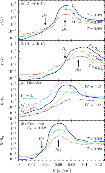
Figure 1: (Color online) (a,b) The MR with an applied magnetic field (a) perpendicular to the surface and (b) parallel to the surface. The blue curve (highest at large fields) is at low temperature, yellow intermediate and red high temperature. The arrows highlight the critical field $B_{\text{C}}$ and the maximum resistance field $B_{\text{M}}$. The points (i - vi) denote the magnetic fields where the current maps of Fig. 3 were evaluated. The perpendicular MR for four different amplitudes of disorder is shown in (c), and with Coulomb repulsion in (d).

In the following we first recover the main experimental results and study how the microscopic variables affect the resistance. We then construct a detailed map of the current flow through the system to uncover the microscopic mechanism that drives the MR peak. First, in Fig. 1(a) we depict the resistance at several temperatures for a sample of size $L_{\text{x}}=21a$ ($\hat{x}$ is the direction of the applied potential), $L_{\text{y}}=11a$, and $L_{\text{z}}=2a$. The interaction strength is $U=2t$, the onsite disorder has width $W=0.5t$, the average density is at $41\%$ filling, and initially there are no long-range repulsive interactions, $U_{\text{C}}=0$. Throughout we set $k_{\text{B}}=1$. At zero magnetic field, the resistance of the SC state is solely the lead-SCR contact resistance. Increasing the magnetic field perpendicular to the surface drives a SCR-insulator transition, around $B_{\text{C}}\simeq 0.04$, in units of (electron) flux quantum per square $[hc/ea^{2}]$, manifested in the reversal of the temperature dependence of the resistance. Above the transition the system displays, in agreement with experiment MR , a peak resistance (at the field $B_{\text{M}}\simeq 0.07$) that is over a hundred times the normal state resistance. This feature consistently emerges for several different statistical configurations of disorder, with the peak resistance varying by a factor of approximately ten. On changing the direction of the (orbital) magnetic field from normal to lying in the plane of the sample (Fig. 1(b)), both $B_{\text{C}}$ and $B_{\text{M}}$ shift to higher fields, with a slight decrease in the magnitude of the MR peak, in complete agreement with recent experiments Johansson11 .

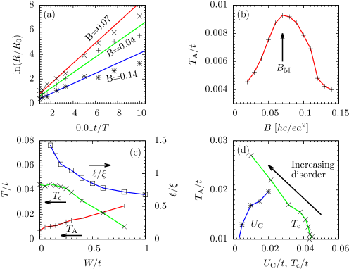
Figure 2: (Color online) (a) The temperature dependence of the resistance at three values of the magnetic field. (b) The activation energy $T_{\text{A}}$ with magnetic field. (c) The activation energy $T_{\text{A}}$ (pluses, red), superconducting transition temperature $T_{\text{c}}$ (crosses, green), and ratio of mean free path $\ell$ to coherence length $\xi$ (squares, blue) with disorder. (d) $T_{\text{A}}$ vs $T_{\text{c}}$ and screened Coulomb interaction $U_{\text{C}}$ for different disorder levels.

We now explore how the MR varies with the parameters of the system. Firstly, in Fig. 1(c) we focus on one specific realization of disorder but increase its amplitude. At low disorder, $W=0.1t$, the magnetic field suppresses the SC state, but there is no MR peak. On increasing the magnitude of the disorder to $W=0.2t$ a peak in the resistive curve emerges at $B\approx 0.09$. (Interestingly, the peak emerges approximately when the mean free path $\ell$ becomes smaller than the coherence length $\xi$, Fig. 2(c).) As disorder is further increased both the SC transition and MR peak shift to lower magnetic fields Siemons08 . In agreement with experiment, the MR peak persists even when the SC phase is suppressed at zero field ($W=0.5t$ and $W=t$), until the peak is extinguished at large enough disorder ($W=2t$). Fig. 1(d) demonstrates that the MR peak becomes more dramatic with increasing Coulomb repulsion, as the MR peak increases by two orders of magnitude. The enhancement of the MR peak by both disorder and Coulomb repulsion points towards a Coulomb blockade mechanism.

(i) $B=0.06hc/ea^{2}$, $T=0.04t$	(ii) $B=0.07hc/ea^{2}$, $T=0.04t$	(iii) $B=0.08hc/ea^{2}$, $T=0.04t$
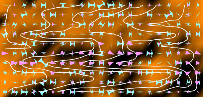
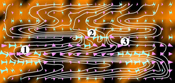
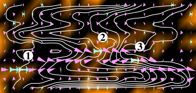
(iv) $B=0.09hc/ea^{2}$, $T=0.04t$	(v) $B=0.08hc/ea^{2}$, $T=0.02t$	(vi) $B=0.08hc/ea^{2}$, $T=0.08t$

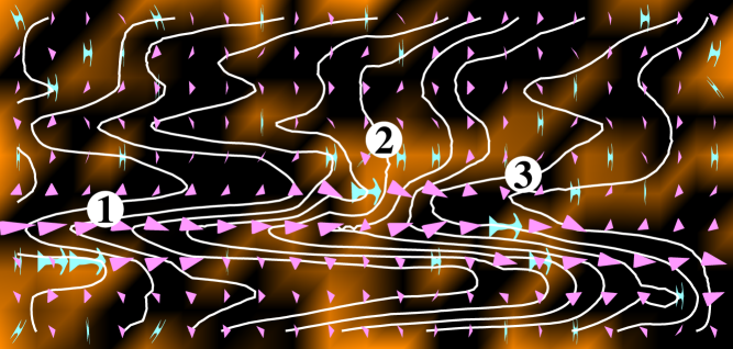
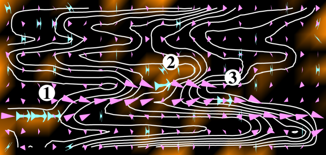
Figure 3: (Color online) Current maps at six values of the normal magnetic field shown in Fig. 1(a). The net current flow is from left to right. The cyan darts show supercurrent and magenta pointers normal current direction and magnitude; their magnitude is renormalized in each map according to the maximum local current flow. The white lines show equi-chemical potential lines across the sample (ten lines correspond to the full potential drop between the two leads), and the background shading depicts the magnitude of the local superconducting order parameter ranging from strong (orange) to zero (black). The labels (1) to (3) highlight three points of special interest.

Fig. 2(a) depicts the temperature dependence of the resistance for several values of magnetic field, which demonstrate an activated behavior, $R=R_{0}\exp(T_{\text{A}}/T)$. The activated behavior, and the peak of the activation temperature $T_{\text{A}}$ at the field $B_{\text{M}}$ (Fig. 2(b)) agrees with experimental observations MR . $T_{\text{A}}$ increases with disorder (Fig. 2(c)) and with repulsive interactions (Fig. 2(d)), consistent with the enhancement of the MR peak by these parameters (Fig. 1(c) and (d)). The critical temperature $T_{\text{C}}$ at which SC correlations are suppressed at zero-field on the other hand falls with disorder. In Fig. 2(d) this gives us an inverse linear dependence of $T_{\text{A}}$ on $T_{\text{C}}$, similar to that seen in experiment MR .

So far we have demonstrated that the calculation reproduces the phenomenology of the experimental observations and hinted that activated transport through a blockade region drives the rise of the resistance. We now take advantage of our ability to probe the evolution of the local currents and chemical potentials with applied magnetic field (Fig. 3 and comprehensively in Fig. S2) to pinpoint the physical processes behind this behavior. Below the critical field, $B_{\text{C}}=0.04$, Fig. S2 shows that no voltage drops across the sample, though the current flow, consisting of Cooper pairs, becomes nonuniform. As the field increases, ($B=0.06$, Fig. 3(i)), there is no longer long-range SC coherence across the system, and current crossing the system changes its nature between SC and normal. Above this field the current has to traverse normal areas of the sample, and as their density increases with magnetic field, the resistance rises. As the field increases further ($B=0.07$, Panel (ii)), the disorder induces specific channels of transport – the current starts as SC, changes into normal current around point (1) and then splits towards points (2) and (3) where it reverts to Cooper pairs, only to change back into normal current as it enters the right-hand lead. At this magnetic field, near the maximal value of the resistance, there are approximately equal contributions to the current from electrons and from Cooper pairs. With increasing field ($B=0.08$, Panel (iii)) the SC areas (2) and (3) shrink and become the main source of voltage drop and resistance in the sample. A larger field ($B=0.09$, Panel (iv)) suppresses the SC correlations, lowering the resistance of the weak links and the overall the resistance. This decrease is, in fact, an interplay of two phenomena – larger SC areas do not serve as weak links (see point (1) in Fig. 3(iii)), but as they shrink with increasing magnetic field the resistance associated with them increases significantly (see point (1) in Fig. 3(iv)). At the same time small SC areas, that gave a significant contribution to the resistance (point (3) in these two panels) become normal and the overall resistance decreases. A much larger magnetic field (Fig. S2) suppresses superconductivity almost completely, giving rise to a uniform drop of voltage across the sample and a significantly lower resistance. Similar behavior has been obtained in the presence of repulsive Coulomb interactions (not shown).

To explore the origin of the Arrhenius behavior panels (v) and (vi) depict the current flow at $B=0.08$ at lower and higher temperatures than Panel (iii). At point (1) we see direct evidence of the activated transport: on lowering the temperature (Panel (v)) more potential is dropped across the weak SC link, whereas with increasing temperature (Panel (vi)) the potential dropped across this weak link falls. The effect of the weak link is so profound that in the hotter panel (vi) despite the reducing SC order more supercurrent flows as the electrons no longer skirt around the SC island as they did in Panel (v). Interestingly at other places in the sample we see the more conventional effect of temperature suppressing superconductivity, for example at point (3) the increasing temperature from Panel (v) to Panel (iii) reduces the SC order parameter and the supercurrent.

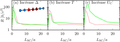
Figure 4: (Color online) The inset of (a) shows the 1D model of a normal state (blue spheres) conducting channel with weak disorder containing a superconducting grain (red prisms) of varying length $L_{\text{SC}}$. In (a) to (c) the red dotted curve is for the same set of standard parameters, and the green solid curves correspond to (a) higher dot order parameter $\Delta=0.9t$, (b) higher temperature $T=0.1t$, and (c) with Coulomb repulsion $U_{\text{C}}=0.02$.

Why would small SC areas serve as weak links and contribute to the increasing resistance? To shed light on this question we studied a toy-model, consisting of a SC island with finite order parameter $\Delta=0.3t$ of length $L_{\text{SC}}$, embedded in disordered normal chain with $\Delta=0$, equal nearest neighbor tunneling, and a temperature $T=0.05t$, shown in the inset of Fig. 4(a). The main figure depicts the resistance of the chain as a function of $L_{\text{SC}}$, with the total chain length fixed. As the SC region becomes shorter, there is a mild increase in the resistance due the increasing length of the resistive normal regions. However, when the SC segment is shorter than $4a$ (similar in size to the SC islands around the resistance peak in Fig. 3(iii)), there is a sudden increase in the resistance of the sample. The resistance peak is enhanced by raising the SC order to $\Delta=0.9t$, (Fig. 4(a)), or increasing temperature to $T=0.1t$ (Fig. 4(b)), demonstrating an activated transport process. This is enhanced on approaching the Anderson limit, where the single particle level-spacing in the SC segment becomes larger than $\Delta$ Anderson . Further corroboration of this picture comes from Fig. 4(a) where the resistance peak emerges at shorter $L_{\text{SC}}$ for higher $\Delta$. Introducing repulsive interactions $U_{\text{C}}=0.05t$ (Fig. 4(c)) has two major effects – there is a larger increase in the resistance and the effect starts at much larger SC segment size, because now the SC gap has to be compared to the Coulomb blockade energy rather than the single-particle spacing. Note that this happens even though this segment is not weakly coupled to the rest of the chain. This is consistent with the description of the MR peak in the two-dimensional systems, where as the SC islands shrink the level spacing, or, more realistically the Coulomb blockade energy becomes of the order of the SC gap, the islands become the weak links and drive up the resistance of the sample.

To conclude, we have demonstrated the emergence of a magnetoresistance peak, starting from a microscopic negative-$U$ Hubbard model. The resistance peak is driven by the competition between Cooper pair and electron transport, where on the weak field side of the peak the normal regions serve as the weak links across the sample, while this role is played by the SC islands on the high field side of the peak, where Coulomb repulsion probably plays a dominant role. These ideas can be further tested by checking the effect of screening by a parallel metallic gate on the peak characteristics. Our picture has some similarities to the heuristic model presented in Ref.Dubi , though there the resistance on the high-field side of the peak was completely associated with the normal electrons, while it is different than the phenomenological approach of Refs.Galitski2005 ; Pokrovsky2010 that discussed the interplay between quasi-particle and Cooper pair transport.

Acknowledgments: GJC acknowledges the financial support of the Royal Commission for the Exhibition of 1851, and the Kreitman Foundation. This work was also supported by the ISF.

I Supplementary material for “Microscopic theory of the magnetoresistance of disordered superconducting films”

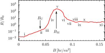
Figure 5: The variation of resistance with an applied magnetic field normal to the surface at $T=0.04t$. $R_{0}=h/e^{2}$ is the resistance quantum. The points (i - xi) denote the magnetic fields where the current maps of Fig. 6 were evaluated, $B_{\text{C}}$ represents the magnetic field where the temperature dependence of the resistance changes sign and $B_{\text{M}}$ the magnetic field at the resistance maximum.

In this supplement we present a comprehensive series of current maps to fully expose the microscopic mechanism driving the breakdown of the superconductor (SC) with applied magnetic field shown in Fig. 5. The maps shown in Fig. 6 cover the entire scope of the SC-insulator transition: maps (i - ii) capture the slight rise of resistance as the superconducting order parameter is reduced but the superconductor remains phase coherent. Maps (iii - vii) outline the loss of phase coherence and formation of weak links through the sample, which drives a dramatic increase in the sample resistance. Finally, in maps (viii - xi) we witness the last remnants of superconductivity being destroyed and the system entering the normal phase with the resistance plateauing out.

(i) $B=0.01hc/ea^{2}$	(ii) $B=0.04hc/ea^{2}$
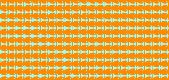
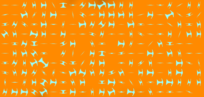
(iii) $B=0.05hc/ea^{2}$	(iv) $B=0.06hc/ea^{2}$
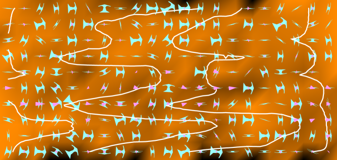
(v) $B=0.07hc/ea^{2}$	(vi) $B=0.08hc/ea^{2}$
(vii) $B=0.09hc/ea^{2}$	(viii) $B=0.10hc/ea^{2}$
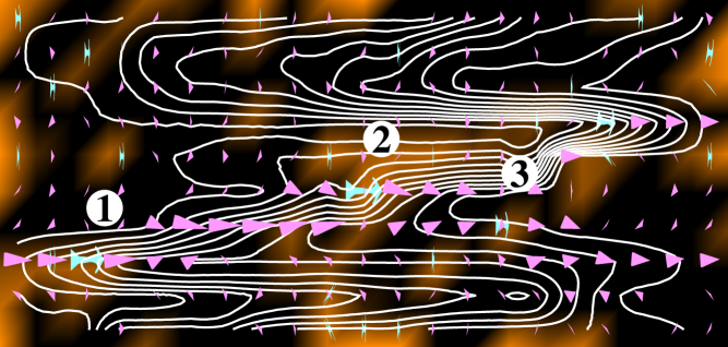
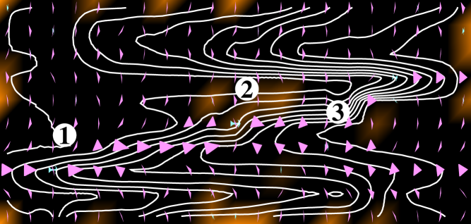
(ix) $B=0.11hc/ea^{2}$	(x) $B=0.12hc/ea^{2}$
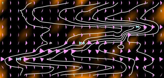
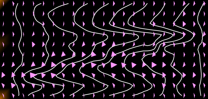
(xi) $B=0.15hc/ea^{2}$	Key

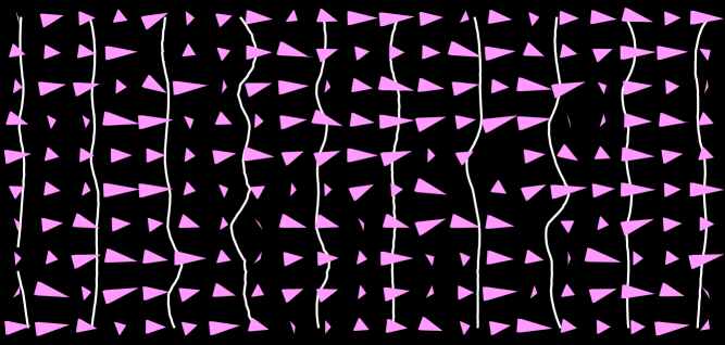
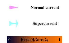
Figure 6: Current maps at eleven values of the magnetic field shown in Fig. 5. The net flow of current is from left to right. As illustrated in the key, the cyan darts show supercurrent and magenta pointers normal current direction and magnitude; their magnitude is renormalized in each map according to the maximum local current flow. The white lines show equi-chemical potential lines across the sample (ten lines correspond to the full potential between the two leads), and background shading depicts the magnitude of the local superconducting order parameter ranging from strong (orange) to zero (black).

We first study the maps (i - ii) that show the current flow when the superconductor is still phase coherent and the resistance is low. The first map (i), corresponds to $B=0.01$, below the critical field $B_{\text{C}}$ (the unit of the magnetic field is the electron quantum flux, $hc/e$, per lattice unit area $a^{2}$). The supercurrent flow is uniform and no voltage is dropped across the sample, but instead the potential is dropped across the lead-superconductor junction. As the field increases to $B=0.04$, (map (ii)), vortices penetrate the sample at points of strong disorder. The supercurrent is no longer uniform as it encircles the vortices, but the sample remains phase coherent and still no potential is dropped across the sample.

Above the critical field $B_{\text{C}}$, the system loses long-range SC coherence and the current changes its nature between SC and normal as it crosses the system. As the field increases to $B=0.05$ (map (iii)) we see the first signs of decay of the order parameter and the current flow becomes normal. With the loss of phase coherence across the system, for the first time potential is dropped across the sample, though around half of the total potential difference is still dropped across the lead-superconductor barriers. Around this field the temperature dependence of the resistance changes sign from superconducting to insulating. As the field increases to $B=0.06$, (map (iv)), normal regions start to form in the sample, and the potential is now dropped mainly across these weak links. As the field increases further to $B=0.07$, (map (v)), the disorder induces specific channels of transport – the current map in Fig. 6 reveals that the current starts as SC, changes into normal current around point (1) and then splits towards points (2) and (3) where it reverts to Cooper pairs, only to change back into normal current as it connects to the right lead. At this magnetic field $B_{\text{M}}$, the maximum in the resistance, there are approximately equal contributions to the current from electrons and from Cooper pairs. On increasing the field to $B=0.08$, (map (iv)), the SC areas (2) and (3) shrink and become the main source of voltage drop and resistance in the sample. A larger field $B=0.09$, (map (v)), suppresses the SC correlations, making area (3) normal, lowering the resistance of that weak link, while at the same time, the SC area (1) shrinks, giving rise to a higher local resistance. Overall the resistance of the sample decreases due to the disappearance of some of the SC island weak links.

Finally, above $B=0.10$ (maps (viii) and (ix)) the SC islands shrink to such extent that the current flows predominantly around them, through the normal areas. With a further increase in the magnetic field to $B=0.12$ (map (x)) only normal current flows through the channels that avoid the residual weak pairing. However, a further increase in magnetic field to $B=0.15$, (map (vi)) suppresses superconductivity almost completely, giving rise to a uniform drop of potential across the sample.

References

- (1) P.W. Anderson, J. Phys. Chem. Solids 11, 26 (1959).
- (2) A.A. Abrikosov, and L.P. Gorkov, Zh. Eksp. Teor. Fiz.36, 319 (1959) [Sov. Phys. JETP 9, 220 (1959)].
- (3) For a recent review , see the relevant chapters in BCS: 50 years, edited by L.N. Cooper and D.E. Feldman, World Scientific, Singapore (2011).
- (4) V.L. Berezinskii, Sov. Phys. JETP 32, 493 (1971); J.M. Kosterlitz and D.J. Thouless, Journal of Physics C: Solid State Physics, 6, 1181, (1973).
- (5) T. Wang, K.M. Beauchamp, A.M. Mack, N.E. Israeloff, G.C. Spalding, and A.M. Goldman, Phys. Rev. B 47, 11619 (1993); V.F. Gantmakher, M.V. Golubkov, J.G.S. Lok, and A.K. Geim, JETP 82, 951 (1996) G. Sambandamurthy, L.W. Engel, A. Johansson, and D. Shahar, Phys. Rev. Lett. 92, 107005 (2004); H.Q. Nguyen, S.M. Hollen, M. D. Stewart, Jr., J. Shainline, Aijun Yin, J.M. Xu, and J.M. Valles, Jr., Phys. Rev. Lett. 103, 157001 (2009).
- (6) G. Sambandamurthy, L.W. Engel, A. Johansson, E. Peled, and D. Shahar, Phys. Rev. Lett. 94, 017003 (2005); V.M. Vinokur, T.I. Baturina, M.V. Fistul, A. Yu. Mironov, M.R. Baklanov and C. Strunk, Nature 452, 613 (2008).
- (7) N. Reyren, S. Thiel, A.D. Caviglia, L. Fitting Kourkoutis, G. Hammerl, C. Richter, C.W. Schneider, T. Kopp, A.-S. Rüetschi, D. Jaccard, M. Gabay, D.A. Muller, J.-M. Triscone, and J. Mannhart, Science 317, 1196 (2007); A.D. Caviglia, S. Gariglio, N. Reyren, D. Jaccard, T. Schneider, M. Gabay, S. Thiel, G. Hammerl, J. Mannhart, and J.-M. Triscone, Nature 456, 624 (2008); J. Biscaras, N. Bergeal, A. Kushwaha, T. Wolf, A. Rastogi, R.C. Budhani, and J. Lesueur, Nature Comm. 1, 1084 (2010).
- (8) G.J. Conduit and Y. Meir, Phys. Rev. B 84, 064513 (2011).
- (9) See, e.g., A. Erez and Y. Meir, Europhys. Lett. 91, 47003 (2010).
- (10) A. Johansson, I. Shammass, N. Stander, E. Peled, G. Sambandamurthy, and D. Shahar, Solid State Comm. 151, 743 (2011).
- (11) W. Siemons, M.A. Steiner, G. Koster, D.H.A. Blank, M.R. Beasley, and A. Kapitulnik, Phys. Rev. B 77, 174506 (2008).
- (12) P.W. Anderson, J. Phys. Chem. Solids 11, 28 (1959); K.A. Matveev and A.I. Larkin, Phys. Rev. Lett. 78, 3749 (1997).
- (13) Y. Dubi, Y. Meir and Y. Avishai, Phys. Rev. B 73, 054509 (2006); Y. Dubi, Y. Meir and Y. Avishai, Nature 449, 876 (2007).
- (14) V.M. Galitski, G. Refael, M.P.A. Fisher, and T. Senthil, Phys. Rev. Lett. 95, 077002 (2005).
- (15) V.L. Pokrovsky, G.M. Falco, and T. Nattermann, Phys. Rev. Lett. 105, 267001 (2010).