Universal scaling in sports ranking

Abstract

Ranking is a ubiquitous phenomenon in the human society. By clicking the web pages of Forbes, you may find all kinds of rankings, such as world’s most powerful people, world’s richest people, top-paid tennis stars, and so on and so forth. Herewith, we study a specific kind, sports ranking systems in which players’ scores and prize money are calculated based on their performances in attending various tournaments. A typical example is tennis. It is found that the distributions of both scores and prize money follow universal power laws, with exponents nearly identical for most sports fields. In order to understand the origin of this universal scaling we focus on the tennis ranking systems. By checking the data we find that, for any pair of players, the probability that the higher-ranked player will top the lower-ranked opponent is proportional to the rank difference between the pair. Such a dependence can be well fitted to a sigmoidal function. By using this feature, we propose a simple toy model which can simulate the competition of players in different tournaments. The simulations yield results consistent with the empirical findings. Extensive studies indicate the model is robust with respect to the modifications of the minor parts.

I Introduction

Most systems in nature have been perceived as a collection of a huge amount of highly interacting units. Although equipped with different components and interactions, different systems could still possess some commonly shared characteristics. Through analyzing the statistical distributions of varieties of empirical quantities, two main patterns of distributions CSN have been found.

For the first one, there is a typical value, around which most quantities distribute tightly clustered NewM , or that is to say, such pattern of distributions are peaked around this typical value. Representative examples include the height of human beings, the speed of cars on the motorway, the intelligence quotient (IQ) test of people, etc. In the traditional IQ test for adults, most people (about 69% of the population) would score in the average range (85-114), a small number (about 26% of the population) would score moderately below average (70-84) and moderately above average (115-129), very high (130 or higher) and very low (below 70) are extremely rare (about 5% of the population).

However, not all quantities could be well characterized by their average values, some would change over an enormous dynamic range, sometimes even many orders of magnitude. Such pattern has absolutely long been familiar with, in the studies regarding the distributions of people’s annual incomes Pareto , word frequencies in text Zipf1 , and city sizes Zipf2 . For the city sizes distribution, if cities are ranked by their population from the largest (rank 1) to the smallest (rank N), it is immediately discovered that, only a small number of cities possess the large population, the majority of cities have the small population. Relationship between rank and city sizes has been found to follow $\ln rank=\alpha+\beta\ln size$, with the slope of the curve $\beta$ being close to -1, which has been well known as Zipf ’s law.

A more general expression of such pattern is the power law distribution, with $p(x)=Ax^{-\beta}$, $A=e^{\alpha}$, and $x$ is the observation of the system. Power law distributions have been considerably widely observed in nature, such as the net worth of the richest individuals in the US NewM , the frequencies of occurrence of words in most human languages NewM ; Zipf1 ; Zipf2 , the frequencies of family names in most cultures FamN , the number of calls received by customs Abello ; Aiello , the number of bytes of data received from computer users Willinger , the number of hits on the web sites Adamic , the number of links to web sites Broder , the number of citations received by papers Price , the sizes of computer files (such as the email address books) CME ; NewM2 , the sizes of earthquakes Earthquake , wars War , craters on the moon Moon and solar flares Solar , the severity of worldwide terrorist attacks Attack , the number of species per genus of mammals Species , the number of sightings of birds of different species Bird , the sales of books Book , and music recordings Cox ; Kohli , etc.

As is well known, ranking is a very interesting and ubiquitous phenomenon in the human society as every one tends to seek the best. By clicking the web pages of Forbes you can find all kinds of rankings, from world’s most powerful people to world’s richest people, from top-paid models to American’s top colleges, etc. Our interest here is certainly not the gossip-like topic, but rather whether there are some common patterns in the vastly different ranking systems. Moreover, if yes, can we understand the formalism of such patterns? To facilitate our study we choose a specific kind of ranking systems, sports ranking, in which data are more suitable for analysis. Here players’ performance in attending various competitions will be used as the basis of their respective rankings, in terms of scores and/or prize money. Amazingly we find that the distributions of scores and/or prize money follow universal power-laws, with exponents being nearly identical for different sports fields. The universal scalings can be reproduced by our model in which the key mechanism is concerned with win-loss probability distribution for any pair of players. This win-loss probability distribution has been verified by the empirical data. Our model is found to be robust with respect to the small modifications of minor parts.

II Empirical results of sports ranking systems

To understand how a certain sports ranking system works, let us take tennis as an example. ATP (Association of Tennis Professionals) and WTA (Women’s Tennis Association) are world’s most successful tennis associations for male and female professionals, respectively. To appear on the ranking systems of ATP or WTA, the number of tournaments a player has to play should reach a minimum, say 10. Tournaments have been divided into several categories, such as grand slams, premier tournaments, international tournaments and year-ending tour championships, mainly based on the prize money. For the most important tournaments such as grand slams, the main draw only consists of 128 players. The entry rule is that if you are top-ranked, then you have more chances to attend the important tournaments. On the other hand, players’ good performance will improve their rankings which will in turn entitle them more chances to play tournaments. Since there are so many tournaments each year, for both ATP and WTA, the ranking list of scores and of prize money vary from week to week. Here we are not interested in which specific player is world No.1 in certain sports, but instead the statistical distribution of performance, measured by scores and prize money, of all the member players. What is the form of such a distribution? Is it stable over different time periods? Is it universal?

Our data sets cover 12 different sports fields, such as tennis, golf, snooker, and volleyball, etc. All the data are updated up to February 2011. As the sample size of data is small, we adopt the cumulative distribution to reduce the potential statistical errors.

II.1 Cumulative distribution of scores

A player’s score or prize money is a direct measure of his/her performance in various competitions. The higher the score, the better the performance. The statistical distribution of scores or prize money reflects the profile of the performance of all the members belonging to the same association. Every sports field has its own scoring system, hence the orders of scores are not always at the same level. In order to make the distributions of scores or prize money comparable for different sports fields, we rescale the quantities of interest. That is,

$$R_{S}=S/S_{max},$$ (1)

where $S$ denotes the values of quantities considered, e.g., scores or prize money, and $S_{max}$ is the maximum value of $S$ in the sample, which pertains to the No. 1 player in the ranking list by using $S$.

Cumulative distributions of players’ scores or prize money have been shown in Fig. 1 for 12 different sports ranking systems. Amazingly all the distributions share very similar trend, which can be well fitted to the power-law with an exponential cutoff as below,

$$P_{>}(S)\propto S^{-\tau}exp(-S/S_{c}),$$ (2)

where $\tau$ and $S_{c}$ are critical exponent and size cutoff, respectively. It should also be noticed that for the same field, all the curves collapse with each other. Values of $\tau$ and $S_{c}$ for different sports fields are given in Table 1, where values of $\tau$ range from 0.01 to 0.39, and the counterparts of $S_{c}$, from 0.12 to 0.28.

Table 1: System sizes of 40 samples in the 12 different sports ranking systems, values of the critical exponent $\tau$ and size cutoff $S_{c}$ in the power law with exponential cutoff, p-values for the statistical significance test, and the ratio of the Pareto principle test.

Sports ranking systems	Sizes	$\tau$	$S_{c}$	$p$	ratio
ATP Single	1763	0.31	0.12	0.65	0.79
ATP Double	1516	0.32	0.18	0.52	0.78
ATP Prize Money	1636	0.33	0.13	0.56	0.79
WTA Single	1523	0.39	0.15	0.62	0.78
WTA Double	1028	0.38	0.19	0.75	0.80
WTA Prize Money	1388	0.39	0.12	0.81	0.81
PGA Score	1323	0.16	0.18	0.85	0.82
LPGA Score	734	0.18	0.19	0.82	0.78
PGA Average Score	1323	0.16	0.19	0.76	0.79
LPGA Average Score	734	0.17	0.20	0.82	0.82
ITTF Prize Money Men	1717	0.32	0.17	0.85	0.83
ITTF Prize Money Women	1288	0.32	0.18	0.73	0.82
FIVA Junior Men	105	0.16	0.21	0.86	0.76
FIVA Junior Women	95	0.14	0.20	0.68	0.79
FIVA Senior Men	138	0.13	0.16	0.69	0.78
FIVA Senior Women	127	0.11	0.18	0.92	0.82
FIFA Men	209	0.01	0.19	0.59	0.77
WPBSA Total Score	97	0.11	0.27	0.69	0.83
WPBSA Average Score	97	0.13	0.25	0.58	0.78
BWF Women Single	548	0.12	0.16	0.68	0.80
BWF Women Double	295	0.13	0.18	0.53	0.78
BWF Men Single	833	0.06	0.17	0.62	0.82
BWF Men Double	429	0.08	0.13	0.75	0.81
BWF Mixed Double	407	0.07	0.14	0.63	0.79
FIBA Men	79	0.19	0.20	0.86	0.81
FIBA Women	72	0.18	0.21	0.98	0.83
FIBA Boys	77	0.18	0.23	0.62	0.82
FIBA Girls	72	0.26	0.22	0.85	0.76
FIBA Combined	115	0.23	0.20	0.52	0.81
IBAF Men	78	0.20	0.28	0.96	0.79
FIH Men	73	0.23	0.26	0.86	0.78
FIH Women	68	0.21	0.27	0.83	0.81
IHF Men	52	0.16	0.25	0.68	0.79
IHF Women	46	0.15	0.27	0.69	0.76
FIE Sabre Senior Women	371	0.34	0.25	0.56	0.81
FIE Foil Senior Women	260	0.32	0.23	0.65	0.78
FIE Epee Senior Women	293	0.36	0.24	0.53	0.83
FIE Sabre Senior Men	319	0.32	0.23	0.67	0.78
FIE Foil Senior Men	337	0.30	0.21	0.56	0.82
FIE Epee Senior Men	442	0.28	0.25	0.72	0.81

We employ the Kolmogorov-Smirnov (KS) test to quantify how closely the power laws with exponential cutoffs resemble the actual distributions of the observed sets of samples. Based on the observed goodness of fit, the p-value, which is defined to be the probability that the real data are drawn from the hypothesized distribution, is calculated for each set of sample. The p-values given in Table 1 for the statistical significance test are all much larger than 0.1, thereby we could conclude the power laws with exponential cutoffs are reliable fits to the samples of different sports ranking systems.

The evidence of the power-laws in the sports ranking indicates that there is still significant probability to have superman such as Roger Federer in tennis or Tiger Woods in golf. But the prevalent probability is still the players who do not play in the top form. Unlike the human height system, it seems there is no typical player who plays with average level. The power-laws found here are also different from Zipf’s law in which the critical exponent is -1, much larger than ours (in absolute value).

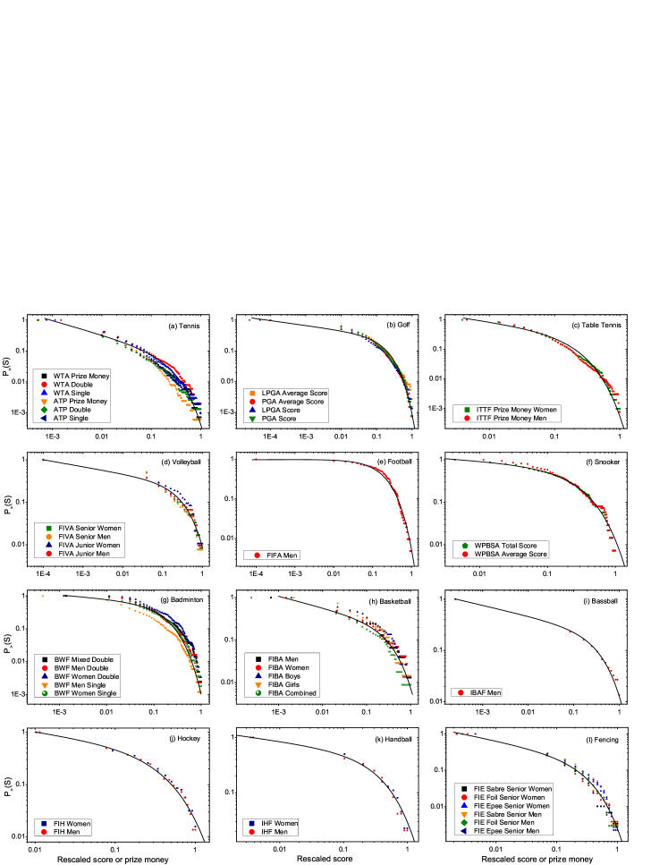
Figure 1: Cumulative distributions of scores and prize money for 12 different sports fields. (a) Tennis: Association of Tennis Professionals (ATP) and Women’s Tennis Association (WTA). (b) Golf: Professional Golfers’ Association (PGA) and Ladies Professional Golf Association (LPGA). (c) Table tennis: International Table Tennis Federation (ITTF). (d) Volleyball: International Federation of Volleyball (FIVB). (e) Football: International Federation of Football Association, commonly known as FIFA. (f) Snooker: World Professional Billiards and Snooker Association (WPBSA). (g) Badminton: Badminton World Federation (BWF). (h) Basketball: International Basketball Federation, more commonly known as FIBA. (i) Baseball: International Baseball Federation (IBAF). (j) Hockey: International Field Hockey Federation (FIH). (k) Handball: International Handball Federation (IHF). (l) Fencing: International Fencing Federation (FIE). All the curves can be fitted to power laws with exponential cutoff, $P_{>}(S)\propto S^{-\tau}exp(-S/S_{c})$, where $\tau$ is the critical exponent and $S_{c}$ is the size cutoff (the turning point). The values of $\tau$ and $S_{c}$ for different sports fields are provided in Table 1.

II.2 Pareto principle

The Pareto principle Pareto2 , also well known as the 80-20 rule, states that, for many events, roughly 80% of the effects comes from 20% of the causes. Pareto noticed that, 80% of Italy’s land was owned by 20% of the population. He carried out such surveys on a variety of other countries further, and to his surprise, the rule was also fulfilled.

The 80-20 rule has also been used to attribute the widening economic inequality, which showed that, the distribution of global income to be very uneven, with the richest 20% of the world’s population controlling 82.7% of the world’s income. The 80-20 rule could be applied to many systems, from the science of management to the physical world.

We also check this rule in the sports ranking systems, it is interesting to find that, 20% players indeed possess approximately 80% scores or prize money of the whole system, the ratios we got in different sports ranking systems are shown in Table. 1, values of the ratios are all very close to 0.8.

II.3 Dependence of win probability on $\Delta$ rank

Here we employ the concept of ”win probability” to describe the chances that a player or a team will win when encountering an opponent. For instance, what is the odds that a No.1 player will top a No.100 player? What is again her chance against No.2? Theoretically, the chance is much higher in the former case than in the latter one. But the result of a competition is not unknown until it is over, which mainly depends on how the player performs at that specific match. However, the win probability could be solely based on the previous performance of a player against a certain opponent, which then can used to predict her future performance against the same opponent. This might have some applications in betting the result of a match. To simplify the case without loss of generality, we relate the win probability solely to the rank difference of a pair of players. Suppose we now have two players A and B, with A having a higher rank. We will then need to know how likely A can beat B when they meet? This quantity is related to but different from the win percentage we usually refer to. The win percentage depicts the percentage of win of a player over all previous encounters. We assume that the win probability only depends on the rank difference between two players. This means, the probability that No.1 beats No.100 is the same as the one that No.100 beats No.200. Hence, we have the following definition,

$$P_{win}(\Delta r)=\frac{N_{win}(\Delta r)}{N_{total}(\Delta r)},$$ (3)

where $\Delta r$ denotes the rank difference (integer), $N_{win}(\Delta r)$ is the total number of win for the higher-ranked players when the rank difference is $\Delta r$, and $N_{total}(\Delta r)$ is the total number of matches in which the rank difference between the pair is $\Delta r$. We here emphasize again that the win probability is the probability that the higher-ranked player will win when two players meet. When $\Delta r$ is small, say 1, it is difficult to judge which player will win, and in this case $P_{win}$ might approximately equal 0.5. When $\Delta r$ is large, for instance 100, $P_{win}$ might approach 1, which means the higher-ranked player is very likely to win.

By using the Head to Head records of ATP and WTA, we find that the dependence of $P_{win}$ on $\Delta r$ can be well fitted to the sigmoidal function as follows,

$$P_{win}=\frac{1}{1+exp{(-a*\Delta r)}},$$ (4)

where $a$ is a parameter dependent on the specific systems. For ATP and WTA, $a$ is 0.021 and $0.032$, respectively. The existence of fluctuations is quite natural since even Roger Federer will not win all the matches. The value of $a$ can still tell us some information about how competitive that certain sports is. The smaller $a$ is, the more competitive the sports will be. Let us take WTA and ATP as two examples. When $\Delta r$ is 30, the win probability for WTA is nearly 0.7, while the counterpart for ATP is 0.65. This means the game is more unpredictable in ATP than in WTA. It is not strange since men’s game is more competitive than women’s. We of course wish to test the empirical finding by checking data from other sports fields, but not so many data are available as far as we know. Despite this, this finding will play a key role in our model to follow.

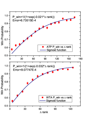
Figure 2: Dependence of win probability on $\Delta r$ of the players for ATP and WTA, which can be well fitted to the sigmoidal function $P_{win}=1/(1+exp{(-a*\Delta r)})$.

III A simple toy model of sports ranking systems

What is the origin of the universal scaling in different sports systems? Of course, there have been so many approaches which can explain the origin of power-laws. Some mechanisms or theories are elegant, e.g., random walks NewM , self-organized criticality (SOC) Bak , etc. It is, however, difficult to try to apply these frameworks to sports ranking systems. We propose a simple toy model, inspired by tennis. Of course, the model may not suit any sports field but does have some general implications. Most importantly, our model can reproduce robust power-laws without having to introduce additional parameters.

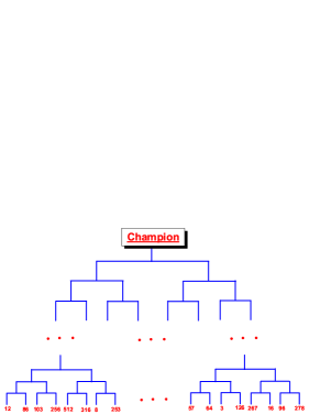
Figure 3: A cartoon of a draw sample. After each round, half players will be eliminated, the numbers ”12, 86 …” denote the ranks of the players.

The rules of the model are defined in the following way,

(1) $2^{N}$ players are ranked from 1 to $2^{N}$, being assigned random scores drawn from a Gaussian distribution.

(2) For each tournament, all the players have entry permission. Therefore the draw will include $2^{N}$ players and in total $N$ rounds. At each round, half of the players will be eliminated when they lose. The rest will enter the next round. The losers at round $n$ will gain score $2^{(n-1)}$. The final champion wins score $2^{N}$.

(3) The key mechanism is to decide which one will lose for a given pair of players. Here our empirical finding will be employed. Namely, when two players meet, the probability that the higher-ranked player will top the lower-ranked opponent is given by $1/(1+exp(-a*\Delta r))$, where $\Delta r$ is their rank difference, as before.

(4) A new tournament opens up and a new draw is made.

In principle, there is only one parameter in our model, that is $a$. We can simply call it competition strength. Of course, there are some shortcomings in the model. First, in the actual tournaments not all the players will be accepted. In grand slams there are only 128 players. Second, tournaments can be divided into many categories and may consist of different players. Third, the scoring systems for different tournaments are a little different. For grand slams the scores and prize money are much higher than other tournaments, if the players are eliminated at the same round. We certainly can add these issues into our model in order to test the resilience of the model. At the moment we do not wish to complicate the model by introducing additional parameters. What we need here is a skeleton which may allow us to understand some key features of the specific systems. Namely, if the power-laws with exponential cutoffs can be reproduced through our model, then it is a feasible model. We need not to care about other minor issues.

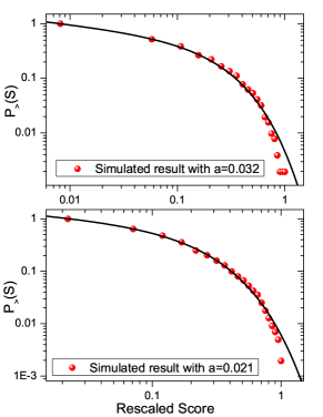
Figure 4: Cumulative distribution of scores from the simulation. For these two samples, number of players $N_{p}=2048$, and number of total tournaments $N_{t}=128$, with $P_{win}=1/(1+exp(-a*\Delta r))$, $a=0.032$ and $0.021$, respectively.

IV Simulation results and discussions

The most important parameter in our model is $a$, the so-called competition strength. The number of players $N_{p}$ and the number of tournaments $N_{t}$ only have finite-size effects. It is natural to check the dependence of the simulation results on these parameters, which can reflect the resilience of our model.

First of all, we need to test whether the model can reproduce the power-laws of the cumulative distribution of scores. In Fig. 4, $N_{p}$ equals 2048, and $N_{t}$ is 128, while win probability, $P_{win}=1/(1+exp(-a*\Delta r))$, with $a=0.021$ and $0.032$, as given by the empirical data of ATP and WTA, respectively. We find that, the cumulative distributions of scores given by the simulations indeed follow the power-law distributions with exponential cut-off, $P(S)\propto S^{-\tau}exp(-S/S_{c})$, with $\tau=0.2,0.22$, $S_{c}=0.23,0.19$, respectively for these two samples. Here we notice that the values of the parameters are very close to what are obtained from the experimental data.

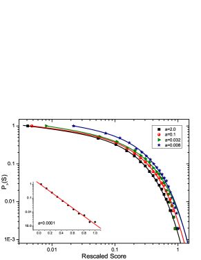
Figure 5: Influence of the critical parameter $a$ on the final cumulative scores distributions, values of $a$ ranging from 0.0001 to 2.0.

In the formula of win probability, smaller values of $a$ correspond to more intensive competition. For instance, when $a=0.0001$, $P_{win}\leqslant 0.525$ for $\Delta r\leqslant 1000$, which means higher-ranked player only has slightly more chances than the lower-ranked player to win the match between them. While larger values of $a$ suggest that the higher ranked players would win the match with a much larger probability. For example, when $a=2.0$, $P_{win}\geqslant 0.88$ for $\Delta rank\geqslant 1$.

Figure 6: Simulation result of the cumulative scores distributions for different number of tournaments, with $N_{t}$=64, 128, and 256.

Thus here, to analyze the influence of win probability, we simulated our models with different values of $a$, $0.0001\leqslant a\leqslant 2.0$. From Fig. 5, we can find that the cumulative scores distributions change from the power laws with exponential cutoff to exponential. Since when $a$ is very small, such as $a=0.0001$, all players nearly win the match randomly, thus the cumulative probabilities of the scores approximately like $1$, $1/2$, $(1/2)^{2}$, …, which results the exponential format.

For different number of tournaments, $N_{t}=64,128$ and $256$, the cumulative distributions of scores are shown in Fig. 6, as seen, one could discover, all the cumulative distributions of scores are power- laws with exponential cutoff, values of the critical exponents $\tau$ and size cutoff $S_{c}$ are also very close to those of the empirical results.

In statistical physics, in order to determine the validity of the statistical approach, we often take the thermodynamic limit, in which the number of components $N$ tends to infinity Finite1 . However, in real world networks, the number of vertices or agents can never be that large, this makes the factor of finite size of paramount importance. For example, even the largest artificial net, the World Wide Web, whose size will soon approach $10^{11}$ Web pages, also shows qualitatively strong finite-size effects Finite2 .

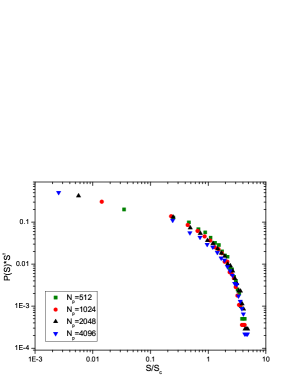
Figure 7: Finite size effects analysis of the simulation results, $N_{p}$=512, 1024, 2048 and 4096.

Therefore, here, in order to test the influence of the finite size effect on the final cumulative scores distribution, we considered the transformed score distribution $P(S)*S^{\tau}$ versus $S/S_{c}$, where $S_{c}$ is the characteristic size cutoff. For four different system sizes, such relationships were shown in Fig. 7, which suggest that, the tails of the four curves almost collapsed with each other, thereby, we can conclude the finite size effect is almost negligible.

V Conclusion

In summary, to characterize the intrinsic common features and underline dynamics of ranking systems, we carry out the investigations in an applicable and specific kind of ranking systems, the sports ranking systems, the main results are: (i) The universal scaling law is extensively found in the distributions of scores and/or prize money, in addition, values of the critical exponents are close to each other for 40 samples of 12 sports ranking systems. (ii) Players’ scores are discovered to obey the Pareto principle, which means, 20% of players approximately possess 80% of total scores of the whole system. (iii) Win probability is introduced to describe the chance that a player or a team will win when meeting an opponent, we simply relate the win probability solely to the rank difference $\Delta r$, for tennis sport, the win probability has been empirically verified to follow the sigmoid function, $P_{win}=1/(1+exp{(-a*\Delta r)})$. (iv) By employing the empirical features of win probability, we proposed a simple toy model to simulate the real process of the sports systems, the universal scaling could be well reproduced by our model, moreover, this result is robust when we change the values of parameters in the model.

We are expecting to find such similar scaling laws in other ranking systems, and we hope all these results and methods could be well applied to analyzing any type of paired competitions, or solving some practical problems in the ranking systems.

References

- (1) Clauset A, Shalizi CR, and Newman MEJ (2009) Power-law distributions in empirical data. SIAM Review 51(4): 661-703.
- (2) Newman MEJ (2005) Power laws, Pareto distributions and Zipf’s law. Contemporary Physics 46(5): 323-351.
- (3) Pareto V (1896) Cours d’Economie Politique. Genève: Droz.
- (4) Zipf GK (1932) Selected Studies of the Principle of Relative Frequency in Language. Cambridge, MA.: Harvard University Press.
- (5) Zipf GK (1949) Human Behavior and the Principle of Least Effort. Cambridge, MA: Addison-Wesley.
- (6) Zanette DH and Manrubia SC (2001) Vertical transmission of culture and the distribution of family names. Physica A 295: 1-8.
- (7) Abello J, Buchsbaum A and Westbrook J (1998) A functional approach to external memory graph algorithms. Proceedings of the 6th European Symposium on Algorithms 1461: 332-343.
- (8) Aiello W, Chung F. and Lu L (2000) A random graph model for massive graphs. Proceeding of the 32nd Annual ACM Symposium on Theory of Computing 171-180.
- (9) Willinger W and Paxson V (1998) Where Mathematics meets the Internet. Notices of the American Mathematical Society 45: 961.
- (10) Adamic LA and Huberman BA (2000) The nature of markets in the World Wide Web. Quarterly Journal of Electronic Commerce 1: 512.
- (11) Broder A, Kumar R, Maghoul F, Raghavan P, Rajagopalan S, Stata R, Tomkins A and Wiener J (2000) Graph structure in the Web. Computer Networks 33: 309.
- (12) Price DJdeS (1965) Networks of scientific papers. Science 149: 510-515.
- (13) Crovella ME and Bestavros A (1996) Self-similarity in World Wide Web traffic: Evidence and possible causes. Proceedings of the 1996 ACM SIGMETRICS Conference on Measurement and Modeling of Computer Systems 148-159.
- (14) Newman MEJ, Forrest S and Balthrop (2002) Email networks and the spread of computer viruses. Phys. Rev. E 66: 035101
- (15) Gutenberg B and Richter RF (1944) Frequency of earthquakes in california. Bulletin of the Seismological Society of America 34: 185-188.
- (16) Roberts DC and Turcotte DL (1998) Fractality and selforganized criticality of wars. Fractals 6: 351-357.
- (17) Neukum G and Ivanov BA (1994) Crater size distributions and impact probabilities on Earth from lunar, terrestial-planet, and asteroid cratering data. Hazards Due to Comets and Asteroids, University of Arizona Press, Tucson, AZ 359-416
- (18) Lu ET and Hamilton RJ (1991) Avalanches of the distribution of solar flares. Astrophysical Journal 380: 89-92.
- (19) Clauset A, Young M and Gleditsch KS (2007) On the Frequency of Severe Terrorist Events. Journal of Conflict Resolution 51: 58.
- (20) Willis JC and Yule GU (1922) Some statistics of evolution and geographical distribution in plants and animals, and their significance. Nature 109: 177-179.
- (21) North American Breeding Bird Survey, Results and Analysis, 1966-2003.
- (22) Hackett AP (1967) 70 Years of Best Sellers, 1895-1965. R. R. Bowker Company, New York.
- (23) Cox RAK, Felton JM, and Chung KC (1995) The concentration of commercial success in popular music: an analysis of the distribution of gold records. Journal of Cultural Economics 19: 333-340.
- (24) Kohli R and Sah R (2003) Market shares: Some power law results and observations. Working paper 04.01, Harris School of Public Policy, University of Chicago.
- (25) Pareto, Vilfredo; Page, Alfred N. (1971), Translation of Manuale di economia politica (”Manual of political economy”), A.M. Kelley, ISBN 9780678008812
- (26) Bak P, Tang C, and Wiesenfeld K (1987), Self-organized criticality: An explanation of the 1/f noise. Physical Review Letters 59: 381-384.
- (27) Toral R and Tessone CJ (2007) Finite size effects in the dynamics of opinnion formation. Commun. Comput. Phys. 2: 177-195.
- (28) Dorogovtsev SN, Goltsev AV and Mendes JFF (2008) Critical phenomena in complex networks. Rev. Mod. Phys. 80: 1275-1335.