Localized Geometric Query Problems

Abstract

A new class of geometric query problems are studied in this paper. We are required to preprocess a set of geometric objects $P$ in the plane, so that for any arbitrary query point $q$, the largest circle that contains $q$ but does not contain any member of $P$, can be reported efficiently. The geometric sets that we consider are point sets and boundaries of simple polygons.

Keywords: Largest empty disk, query answering, medial axis, computational geometry

1 Introduction

Largest empty space recognition is a classical problem in computational geometry, and has applications in several disciplines like database management, operations research, wireless sensor network, VLSI, to name a few. Here the problem is to identify an empty space of a desired shape and of maximum size in a region containing a set of obstacles. Given a set $P$ of $n$ points in $\mathbb{R}^{2}$, an empty circle, is a circle that does not contain any member of $P$. An empty circle is said to be a maximal empty circle (MEC) if it is not fully contained in any other empty circle. Among the MECs, the one having the maximum radius is the largest empty circle. The largest empty circle among a point set $P$ can easily be located by using the Voronoi diagram of $P$ in $O(n\log n)$ time [32].

Although a lot of study has been made on the empty space recognition problem, surprisingly, the query version of the problem has not received much attention. The problem of finding the largest empty circle centered on a given query line segment has been considered in [3]. The preprocessing time, space and query time complexities of the algorithm in [3] are $O(n^{3}\log n)$, $O(n^{3})$ and $O(\log n)$, respectively. In practical applications, one may need to locate the largest empty circle in a desired location. For example, in the VLSI physical design, one may need to place a large circuit component in the vicinity of some already placed components. Such problems arise in mining large data sets as well, where one of the objectives is to search for empty spaces in data sets [23]. In [12], Edmonds et al. formalized the problem of finding large empty spaces in geometric data sets. In particular, they studied the problem of finding large empty rectangles in data sets.

An important problem in this context is the circular separability problem. Two planar sets $P_{1}$ and $P_{2}$ are circularly separable if there is a circle that encloses $P_{1}$ but excludes $P_{2}$. O’Rourke et al. [27] showed that the decision version of the circularly separability of two sets can be solved in $O(n)$ time using linear programming. Furthermore, they show that a smallest separating circle can be found in $O(n)$ time while the computation of the largest separating circle needs $O(n\log n)$ time. Detailed study on circular separability problem can be found in [7, 8, 13, 27]. Boissonnat et al. [8] proposed a linear-time algorithm for solving the decision version of circular separability problem where the sets $P_{1}$ and $P_{2}$ are simple polygons, and the algorithm outputs the smallest separating circle. They also consider the query version of this problem where the objective is to preprocess a convex polygon $P$ such that given a query point $q$ and a query line $\ell$, report the largest circle inside $P$ that contains $q$ and does not intersect $\ell$. The preprocessing time and space complexities of their proposed algorithm are both $O(n\log n)$, and the query can be answered in $O(\log n)$ time. They also showed that a convex polygon $P$ can be preprocessed in $O(n)$ time and space such that for a query set $S$ of $k$ points, the largest circle inside $P$ that encloses $S$ can be computed in $O(k\log n)$ time.

In addition to empty circles, empty rectangles have also been studied. We introduced the query version of the maximal empty rectangle in [1]. The problem entails preprocessing a set of $n$ points such that, given a query point $q$, the largest empty rectangle containing $q$ can be reported efficiently. We gave a solution with query time $O(\log n)$ with preprocessing time and space being $O(n^{2}\log n)$ and $O(n^{2})$, respectively. Recently, Kaplan et al. [19] improved the preprocessing time and space complexities to $O(n\alpha(n)\log^{4}n)$ and $O(n\alpha(n)\log^{3}n)$, respectively, while the query time has increased to $O(\log^{4}n)$. Here $\alpha(n)$ is the inverse Ackermann function.

1.1 Our Results

In this paper, we study the query versions of the maximum empty circle problem (QMEC). The following variations are considered.

• Given a simple polygon $P$, preprocess it such that given a query point $q$, the largest circle inside $P$ that contains the query point $q$ can be identified efficiently.

• Given a set of points $P$, preprocess it such that given a query point $q$, the largest circle that does not contain any member of $P$, but contains the query point $q$ can be identified efficiently.

Our results are summarized in Table 1.

Table 1: Complexity results for different variations of largest empty space query problem

Geometric set	Preprocessing	Space	Query time
	time
Simple Polygon	$O(n\log^{2}n)$	$O(n\log n)$	$O(\log n)$
Point Set	$O(n^{3/2}\log^{2}n)$	$O(n^{3/2}\log n)$	$O(\log n\log\log n)$
Point Set	$O(n^{5/3}\log n)$	$O(n^{5/3})$	$O(\log n)$

We believe that our work will motivate the study of new types of geometric query problems and may lead to a very active research area. The main theme of our work is to achieve subquadratic preprocessing time and space, while ensuring polylogarithmic query times. The results in this paper, improve upon the results in our previous work [1]. Very recently, Kaplan and Sharir [20] provided a solution to the QMEC problem for point sets that only requires $O(n\log^{2}n)$ time and $O(n\log n)$ space for preprocessing. Their query times, however, are $O(\log^{2}n)$.

1.2 Organization of the paper

In Section 2, as a preliminary requisite, we describe a way to answer QMEC query for the case of convex polygons. The same bounds have been achieved by Boissonnat et al. [8], but our solution is slightly different and serves as the basis for solving the QMEC problem on simple polygons. In Section 3, we present the QMEC problem for simple polygons with $n$ vertices. The preprocessing time and space complexities are $O(n\log^{2}n)$ and $O(n\log n)$ respectively, and the query answering time is $O(\log n)$. In Section 4, we consider the same problem on a set $P$ of $n$ points in $\mathbb{R}^{2}$. We present two algorithms (cf. Table 1). Our first algorithm uses the concept of planar separators [22] on the underlying planar graph corresponding to the Voronoi diagram of $P$. It solves the QMEC problem on $P$ with $O(n^{3/2}\log^{2}n)$ preprocessing time and $O(n^{3/2}\log n)$ space. Here, the queries can be answered in $O(\log n\log\log n)$ time. Our second algorithm (cf. Section 4.4) uses the $r$-partitioning [14] of planar graphs. With a suitable choice of $r$, the query time is only $O(\log n)$, an improvement over our first algorithm. However, the preprocessing time and space increase to $O(n^{5/3}\log n)$ and $O(n^{5/3})$, respectively.

2 Preliminaries: QMEC problem for a convex polygon

Let $P$ be a convex polygon and $\{p_{1},p_{2},\ldots,p_{n}\}$ be its vertices in counter-clockwise order. Our objective in this section is to preprocess $P$ such that given an arbitrary query point $q\in P$, the largest circle $C_{q}$ containing $q$ inside the polygon $P$ can be reported efficiently. Note that, the locus of the centers of all the maximally empty circles (MECs) inside $P$ is defined to be the medial axis $M$ of $P$. Let $c$ be the center of the largest MEC inside $P$ (see Figure 1(a)). The medial axis of a convex polygon consists of straight line segments and can be viewed as a tree rooted at $c$ [11]. To avoid confusion with the vertices of the polygon, we call the vertices of $M$ as nodes. Note that, the leaf-nodes of $M$ are the vertices of $P$. Let us denote an MEC of $P$ centered at a point $x\in M$ as ${\tt MEC}_{x}$ and let $A_{x}$ be the area of ${\tt MEC}_{x}$.

In [8], a planar map of circular arcs is constructed by drawing the MEC at each node of $M$ in $O(n)$ time and space. The problem of finding $C_{q}$ reduces to the point location problem in the associated planar map. These point location queries can be answered in $O(\log n)$ time. We propose an alternative solution (with the same complexity results as in [8]) because our new technique plays a basic role in solving the problem when $P$ is a simple polygon (cf. Section 3.2). We use the fact that the medial axis $M$ is a tree, and then use the level-ancestor queries [6] on $M$.

Figure 1: (a) Illustration of Lemma 1, and (b) partition of $P$.

Lemma 1

[8] As the point $x$ moves from the center $c$ of the largest MEC along the medial axis towards any vertex $p_{i}\in P$ (leaf node of $M$), $A_{x}$ decreases monotonically.

Lemma 2

The polygon $P$ can be preprocessed in $O(n)$ time such that given any arbitrary query point $q$, a point $x$ on $M$ such that ${\tt MEC}_{x}$ contains $q$ can be reported in $O(\log n)$ time.

Proof

The medial axis $M$ subdivides $P$ into $n$ convex faces such that each face $P_{i}$ consists of an edge $p_{i}p_{i+1}$ from $P$ and a convex chain of edges from $M$ connecting $p_{i}$ to $p_{i+1}$ (see Figure 1(b)). In the preprocessing phase, we perform the following steps.

1. Compute the medial axis $M$ of $P$, which is a tree rooted at $c$.

2. Compute the subdivision in $O(n)$ time. For this we will need $M$, which can be computed in linear time [11].

3. Store the chain of edges associated with each face in an array so that it is amenable to binary searching.

4. Finally, the subdivision can be preprocessed in $O(n)$ time so that the face containing a query point $q$ can be located in $O(\log n)$ time [21].

In the query phase, we perform the following steps.

1. We find the face $P_{i}$ that contains $q$ in $O(\log n)$ time.

2. Recall that exactly one edge $p_{i}p_{i+1}$ of $P$ will be an edge in $P_{i}$. Consider the line $\ell$ through $q$ that is perpendicular to the edge $p_{i}p_{i+1}$. It will intersect an edge in $M$ that is also an edge bounding $P_{i}$; we report that intersection point as $x$. Note that $x$ can be computed in $O(\log n)$ time via binary searching over the chain of medial axis edges bounding $P_{i}$.

We need to prove that ${\tt MEC}_{x}$ indeed encloses $q$. Firstly, note that $\ell$ will intersect the edge $p_{i}p_{i+1}$ internally at a point $t$ because (i) $P_{i}$ is convex and (ii) the two internal angles in $P_{i}$ at $p_{i}$ and $p_{i+1}$ are both acute. Secondly, note that any MEC that goes through $t$ must be tangential to $p_{i}p_{i+1}$, thereby making it unique and centred on $\ell$; more precisely, the MEC that goes through $t$ must be centred at $x$. Finally, from the construction, it is clear that $q$ lies on the diameter of ${\tt MEC}_{x}$, thus proving that that ${\tt MEC}_{x}$ encloses $q$. ∎

Now we will describe how to solve the QMEC problem for a convex polygon. Given a query point $q$ we find (using Lemma 2) the point $x$ on $M$ such that ${\tt MEC}_{x}$ encloses $q$.

Observe (informally for now) that, for any fixed point $q$ inside $P$, the MECs that encloses $q$ are centered on a connected subtree $M^{q}$ of the medial axis $M$. This observation is formally proved in Lemma 3 in the more general setting of simple polygons. Coupling this observation with Lemma 1, we can conclude that $c_{q}$ is the point on $M^{q}$ closest to the root $c$ of $M$. Therefore, we can locate $c_{q}$ by performing a binary search on the path $x\sim c$. We find two consecutive nodes $v$ and its parent $v^{\prime}$ on the path $x\sim c$ such that ${\tt MEC}_{v}$ encloses $q$, but ${\tt MEC}_{v^{\prime}}$ does not. Since the path lies on a tree representing the medial axis $M$, we can use level-ancestor queries [6] for this purpose. After computing $v$ and $v^{\prime}$, the exact location of $c_{q}$ can be computed in $O(1)$ time. Thus, we have the following theorem:

Theorem 2.1

A convex polygon $P$ with $n$ vertices can be preprocessed in $O(n)$ time and space such that, given any arbitrary query point $q\in P$, the largest circle containing $q$ inside $P$ can be reported in $O(\log n)$ time.

3 QMEC problem for simple polygons

Let $P$ be a simple polygon on $n$ vertices. Recall that the medial axis $M$ of $P$ is defined to be the locus of the centers of all circles inside $P$ that touch the boundary of $P$ in two or more points (see, e.g., [11]). While the medial axis of a convex polygon consists only of straight line segments, the medial axis of a simple polygon may additionally contain parabolic arcs [28].

Our approach for solving the QMEC problem uses the fact that $M$ is a geometric tree. Its leaf nodes correspond to the vertices of $P$, and the internal nodes correspond to the points on $M$ such that the MECs centered at each of those points touch three or more distinct points on the boundary of $P$. We denote the set of internal nodes of $M$ as ${\tt N}$. An edge in $M$ is a path between two nodes that does not contain any other node in its interior. Note that a single edge consists of one or more line segments or parabolic arcs.

For any point $x\in M$, we denote the maximal empty circle centered at $x$ in $P$ by ${\tt MEC}_{x}$. A point $x\in M$, that is not a leaf, is said to be a valley (resp., peak) if for a positive $\delta\to 0$, the MECs centered at points in $M$ within distance $\delta$ from $x$ are at least as large as (resp., no larger than) ${\tt MEC}_{x}$ and at least one such MEC is strictly larger (resp., smaller) than ${\tt MEC}_{x}$. Note that a pair of parallel edges in $P$ may induce a pair of peaks or a pair of valleys. In such cases, we only pick one representative peak or valley and discard the other. We use $\Phi$ and $\Theta$ to denote the set of valleys and peaks, respectively. For any $x\in\Phi$, it is easy to observe that ${\tt MEC}_{x}$ touches $P$ in exactly two points diametrically opposed to each other. Otherwise, we can move along a direction to get smaller MECs. As a consequence, a valley can only be in the interior of an edge. Therefore, $\Phi\cap{\tt N}=\emptyset$. On the other hand, $\Theta\subseteq{\tt N}$.

We define a mountain to be a maximal subtree of $M$ that does not contain any valley point (except as its leaves). We partition $M$ by cutting the tree at all the valley points, and generate a set of mountains ${\tt M}=\{M_{1},M_{2},\ldots,M_{|{\tt M}|}\}$ (See Figure 2(a)).

Observation 1

(i) Each valley point is the common leaf of exactly two mountains.
(ii) Each mountain has exactly one peak.
(iii) If a point $x$ moves from a valley point of a mountain towards its peak, the size of ${\tt MEC}_{x}$ increases monotonically.

Proof

Suppose $v$ is a valley point. We have noted earlier that $v$ can only be in the interior of an edge. Therefore, $v$ must be a common leaf between exactly two mountains.

For part (ii), assume that there are two peaks $p_{1}$ and $p_{2}$ in a mountain. Consider the path in $M$ from $p_{1}$ to $p_{2}$ (denoted $p_{1}\sim p_{2}$). Consider the point $x^{*}=\arg\min_{x\in p_{1}\sim p_{2}}{\tt MEC}_{x}$. One can observe that $x^{*}$ will be a valley, implying that $p_{1}$ and $p_{2}$ cannot be in the same mountain.

Consider a point $x$ that moves from a valley of a mountain towards its peak. If the MECs don’t increase monotonically, it is easy to see that a valley point will be encountered. This implies that $x$ has moved into another mountain.∎

(a)

(b)

Figure 2: (a) Partitioning the medial axis $M$ into mountains, and (b) The subtree $M^{q}$ for a query point $q$

At each valley point $x$ of $M$, consider the chord in $P$ connecting the two points at which ${\tt MEC}_{x}$ touches $P$. These chords induced by each $x\in\Phi$ will partition $P$ into a set of sub-polygons $\{P_{1},P_{2},\ldots,P_{|{\tt M}|}\}$ of cardinality equaling the total number of mountains because this partitioning ensures that the portion of $M$ contained in each of these sub-polygons is a mountain containing a single peak.

Given a (query) point $q\in P$, let $M^{q}\subseteq M$ denote the locus of the centers of all possible maximal empty circles in $P$ that enclose $q$ (see Figure 2(b)). The following structural lemma plays a crucial role in designing our algorithm.

Lemma 3

$M^{q}$ is a (connected) subtree of $M$.

Proof

For the sake of contradiction, let us assume that $M^{q}$ is disconnected. Then, there are at least two distinct points $t_{1}$ and $t_{2}$ on the medial axis such that (a) ${\tt MEC}_{t_{1}}$ and ${\tt MEC}_{t_{2}}$ contain $q$, but (b) ${\tt MEC}_{t}$ does not contain $q$ for some $t$ on the path along the medial axis connecting $t_{1}$ and $t_{2}$.

Without loss of generality, we assume that such a $t$ is not a node in $M$. Therefore, ${\tt MEC}_{t}$ touches the simple polygon $P$ at exactly two points, $a$ and $b$. The chord $[a,b]$ partitions $P$ into two polygons $P_{left}$ and $P_{right}$ to the left and right of $[a,b]$ respectively (see Figure  3(a)). Note that, $t$ also partitions the medial axis into two subtrees, $M_{left}$ and $M_{right}$, such that $t_{1}\in M_{left}$ and $t_{2}\in M_{right}$. For the rest of the proof, we use ${\tt MEC}_{t}$ and $P_{left}$ to denote the region enclosed by them. We now claim that

$${\tt MEC}_{t_{1}}\subset P_{left}\cup{\tt MEC}_{t}=P\setminus(P_{right}\setminus{\tt MEC}_{t}).$$ (1)

Figure 3: Proof of Lemma 3: (a) the general case, and (b) a special case where the points $a$ and $b$ are concave vertices of $P$

To show that Equation 1 holds, we consider the following cases.

Case: ${\tt MEC}_{t_{1}}$ touches $P$ at both $a$ and $b$:

This case is illustrated in Figure 3(b). Here, $a$ and $b$ must be concave vertices that induce a straight line segment edge in the medial axis. Both $t$ and $t_{1}$ are on that edge; in particular, $t_{1}$ will be to the left of $t$. It is now easy to infer that Equation 1 holds.

Case: ${\tt MEC}_{t_{1}}$ touches at most one of $\{a,b\}$:

Let ${\tt MEC}_{t_{1}}$ touch the other point $d\not\in\{a,b\}$ on the boundary of $P$. Clearly, $d\in P_{left}\setminus{\tt MEC}_{t}$. If we assume that ${\tt MEC}_{t_{1}}$ also passes through a point $d^{\prime}\in P_{right}\setminus{\tt MEC}_{t}$, then it is impossible to construct ${\tt MEC}_{t_{1}}$ without properly enclosing some point outside $P$. Therefore, Equation 1 holds.

By symmetry, we can also say that

$${\tt MEC}_{t_{2}}\subset P_{right}\cup{\tt MEC}_{t}=P\setminus(P_{left}\setminus{\tt MEC}_{t}).$$ (2)

Taking the intersection of Equations 1 and 2, we get

${\tt MEC}_{t_{1}}\cap{\tt MEC}_{t_{2}}\subset(P_{left}\cup{\tt MEC}_{t})\cap(P_{right}\cup{\tt MEC}_{t})$
= $(P_{left}\cap P_{right})\cup{\tt MEC}_{t}$ = ${\tt MEC}_{t}$ (since $(P_{left}\cap P_{right})\subset{\tt MEC}_{t}$.

This contradicts our assumption that $q$ falls in ${\tt MEC}_{t_{1}}$ and ${\tt MEC}_{t_{2}}$, but not in ${\tt MEC}_{t}$. ∎

Corollary 1

Let $v\in M$ be such that ${\tt MEC}_{v}$ does not contain $q$. Then $M^{q}$ is contained entirely in one of the subtrees of $M$ obtained by deleting $v$ from $M$.

Corollary 2

Consider two points $u,v\in M$, such that ${\tt MEC}_{v}$ overlaps with ${\tt MEC}_{u}$. Let $\alpha$ be a point in $P$ such that $\alpha\in{\tt MEC}_{v}\cap{\tt MEC}_{u}$. Then $\alpha$ will lie in all MECs centered along the path from $v$ to $u$ in $M$.

Proof

Since ${\tt MEC}_{v}$ overlaps with ${\tt MEC}_{u}$ and $\alpha\in{\tt MEC}_{v}\cap{\tt MEC}_{u}$, both $v$ and $u$ are points on $M^{\alpha}$. The result now follows immediately from Lemma 3. ∎

Before we delve into solving QMEC, in the next three subsections, we define three data structures that we use as building blocks.

3.1 PLiCA: Point location in circular arrangement

The problem is to preprocess a set ${\tt C}=\{C_{1},C_{2},\ldots,C_{n}\}$ of circles of arbitrary radii, so that for any query point $q$ in the plane, we need to quickly report if there exists a circle $C_{i}\in{\tt C}$ such that $q\in C_{i}$. This can be achieved by using the concept of Voronoi diagrams in Laguerre geometry of circles in $\tt C$ [16]. Each cell of the Voronoi diagram is a convex polygon and is associated with a circle in ${\tt C}$. The membership query is answered by performing a point location in the associated planar subdivision. The preprocessing time and space complexities are $O(n\log n)$ and $O(n)$ respectively, and the queries can be answered in $O(\log n)$ time.

3.2 QiM: Query-in-Mountain

Given a mountain $M_{i}\in{\tt M}$, we must preprocess it such that given a query point $q$ inside $P$ such that $M_{i}\cap M^{q}\neq\emptyset$ (and a point $x\in M_{i}\cap M^{q}$), our task is to report the largest MEC centered at a point on $M_{i}$ that contains $q$. Note that if the center moves from $x$ towards the peak of $M_{i}$, the size of the MEC increases monotonically. Thus, we can apply the algorithm proposed in Section 2 for the convex polygon case to identify the largest MEC containing $q$, and centered on $M_{i}\cap M^{q}$. The preprocessing time and space complexities for the mountain $M_{i}$ are both $O(|P_{i}|)$, and the query time is $O(\log|P_{i}|)$, where $|P_{i}|$ denotes the number of edges in the sub-polygon $P_{i}$ that induces $M_{i}$. Since the set of mountains and sub-polygons are partitions of the medial axis $M$ and the polygon $P$, respectively, all the mountains can be preprocessed for the QiM queries in $O(n)$ time.

3.3 QiC: Query-in-Circle (Problem Definition and Bounds)

The QiC is a simplification of the QMEC problem in which, in addition to $P$ and its medial axis $M$, a node $v$ of $M$ is specified as part of the input for preprocessing. We are promised that the query point $q$ will lie inside ${\tt MEC}_{v}$. As in ${\tt QMEC}$, we are to report the largest MEC $C_{q}$ that contains $q$. We defer the details of our solution for the QiC problem to Section 3.6, where we prove the following theorem.

Theorem 3.1

There exists a solution for QiC that takes $O(n\log n)$ time and $O(n)$ space for preprocessing. Queries can be answered in $O(\log n)$ time.

To solve QMEC, we employ a divide-and-conquer strategy that divides the medial axis into smaller pieces. On these smaller pieces, we employ QiC. We remark in Section 3.6 how the solution to the QiC problem on the entire medial axis can be adapted to restricted portions of the medial axis. For now, we note that the preprocessing time and space of QiC scale with the size of the portion of the medial axis that is preprocessed. On a portion $M^{*}$ of the medial axis, the preprocessing time and space are $O(n^{*}\log n^{*})$ time and $O(n^{*})$, respectively, where $n^{*}$ is the number of edges of $P$ that induce the edges in $M^{*}$ (cf. Corollary 4).

Algorithm 1 Preprocessing for QMEC on a Simple Polygon $P$

0:  A simple polygon $P$.

1:  Compute the medial axis $M$ of $P$.

2:  Construct a PLiCA data structure on MECs centered on nodes of $M$.

3:  Construct a secondary PliCA data structure on the MECs centered on valley points of $M$.

4:  Construct a list $(M_{1},M_{2},\ldots)$ of mountains and preprocess each mountain for QiM.

5:  Partition $P$ into sub-polygons $P_{1}$, $P_{2}$, $\ldots$ such that each $P_{i}$ is associated with its corresponding $M_{i}$. (Recall that this can be performed by cutting along diameters of MECs centered on valley points.)

6:  Preprocess $P$ and its sub-polygons (in $O(n)$ time and space) such that, given a query point $q$, the sub-polygon that contains $q$ can be reported efficiently (in $O(\log n)$ time). Call this data structure $D$.

7:  $T\leftarrow$ Decompose($M$).

8:  for each node $t\in T$ do

9:     Let $M^{t}\subseteq M$ be the subtree associated with $t$.

10:     Let $v^{t}$ be the centroid of $M^{t}$ (cf. Lemma 4).

11:     Preprocess ${\tt MEC}_{v^{t}}$ for QiC with the additional promise that the largest empty circle $C_{q}$ that contains query point $q$ is centered on $M^{t}$. Associate this QiC data structure with $t$.

12:  end for

Algorithm 2 Decompose($M$)

0:  A tree $M$ with $n$ nodes.

0:  A divide-and-conquer tree $T$ that decomposes $M$.

1:  if $n=1$ then

2:     return  a tree with the single node.

3:  end if

4:  Find the centroid (cf. Lemma 4) of $M$ that will decompose $M$ into subtrees $M^{1}$, $M^{2}$, $\ldots$

5:  Create a node node with a list child of child pointers.

6:  Associate $M$ with node.

7:  for each subtree $M^{i}$ do

8:     node.child[i] $\leftarrow$ Decompose($M^{i}$).

9:  end for

Algorithm 3 Query phase of QMEC on a simple polygon $P$ with query point $q$

0:  Query point $q$ and all the data structures created in the preprocessing phase. {We can use the PLiCA data structure for the following condition.}

1:  if $q$ falls inside some MEC centered on a node $v$ of $M$ then

2:     {We are in the affirmative case.}

3:     Find the node $t$ in $T$ whose centroid is $v$.{In the next step, $v^{*}$ is the centroid of the subtree of $M$ associated with $t^{*}$.}

4:     Find (in $T$) the farthest ancestor $t^{*}$ of $t$ such that ${\tt MEC}_{v^{*}}$ contains $q$.

5:     $C_{q}\leftarrow$ circle returned by querying the QiC data structure associated with $v^{*}$.

6:     Return $C_{q}$.

7:  else

8:     {We are in the negative case.}

9:     if $q$ falls in some MEC centered on a valley point $p$ then

10:        {$p$ is a valley point connecting exactly two mountains $A$ and $B$.}

11:        $C_{q}$ is the larger of the MECs returned by querying the QiM data structures associated with $A$ and $B$.

12:        Return $C_{q}$.

13:     else

14:        Use data structure $D$ to find the sub-polygon $P^{q}$ that contains $q$.

15:        $C_{q}\leftarrow$ circle returned by querying the QiM data structure associated with $P^{q}$.

16:        Return $C_{q}$

17:     end if

18:  end if

3.4 Preprocessing for the QMEC problem

Algorithm 1 outlines the steps in the preprocessing phase. The first 6 steps are straightforward. Before we explain the subsequent steps, we state (for the sake of completeness) a well-known lemma.

Lemma 4

[18] Every tree $M$ with $n$ nodes has at least one node $v$ whose removal splits the tree into subtrees with at most $\lceil\frac{n}{2}\rceil$ nodes. The node $v$ is called the centroid of $M$.

In line number 7 we call Algorithm 2 (recursively) to build a centroid decomposition tree $T$. We partition using the centroid (cf. Lemma 4) in order to ensure that $T$ is balanced.

The centroid decomposition is constructed in anticipation of the query phase. Suppose $q$ is a query point. If $q$ lies in ${\tt MEC}_{v}$, where $v$ is the centroid associated with the root of ${\tt T}$. Then, we can use the ${\tt QiC}$ attached to the root (in line number 11). If, on the contrary, $q\not\in{\tt MEC}_{v}$, then from Corollary 1 we know that only one of the subtrees rooted at $v$ will contain $M^{q}$, thereby allowing us to recurse into that subtree until we find the centroid whose MEC encloses $q$. To facilitate this recursion, we must provide a way to find the correct subtree to recurse into. For this, we consider the geometry of the polygon $P$. Let ${\tt MEC}_{v}$ touch the polygon $P$ at $k$ ($\geq 3$) points. Consider the partitioning of $P$ into $k$ sub-polygons, apart from the one containing $v$, by inserting chords as shown in Figure 4. These $k$ sub-polygons correspond to the $k$ subtrees of $M$ obtained by removing $v$. It is easy to see now that a point location data structure will suffice. In the query phase, we can simply find the sub-polygon that contains $q$ and recurse into the corresponding subtree.

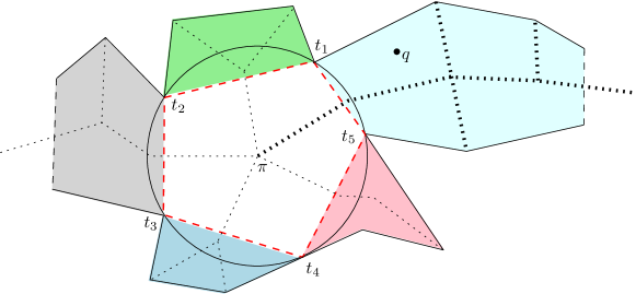
Figure 4: The divide and conquer search structure

In lines 8 to 12, for each node $t$ of $T$ we associate an appropriate subtree $M^{t}$ of $M$ along with the centroid $v^{t}$ of $M^{t}$. Additionally, we will construct a QiC data structure associated with $t$ with the additional promise that the largest empty circle $C_{q}$ that contains query point $q$ is centered on $M^{t}$.

Lemma 5

The time and space required for preprocessing $P$ are $O(n\log^{2}n)$ and $O(n\log n)$, respectively.

Proof

The medial axis $M$ of a simple polygon can be computed in $O(n)$ time [11]. Once we have $M$, the partition of $M$ into mountains, and the associated partitioning of $P$ can be done in $O(n)$ time. The data structure for the planar point location can easily be obtained in $O(n\log n)$ time and $O(n)$ space. The PLiCA data structure for all the MECs centered at the nodes of $M$ requires $O(n\log n)$ time and $O(n)$ space.

Consider a level $\ell$ in the tree $T$. Each node in level $\ell$ implements the QiC data structure on a portion of the medial axis that is disjoint from the portion addressed by other QiC implementations in the same level. Therefore, the preprocessing times and spaces of all QiCs at any level $\ell$ is $O(n\log n)$ and $O(n)$ respectively. Since there are $O(\log n)$ levels in $T$, the total preprocessing time and space for all QiCs is $O(n\log^{2}n)$ and $O(n\log n)$, respectively. ∎

3.5 QMEC query

As discussed in Algorithm 3, in the query phase with a point $q$, we first test whether $q$ lies in the MEC centered at any node $v$ of the medial axis. This can be performed using the PLiCA data structure (see Subsection 3.1) built over the set of MECs centered at all the nodes in $M$. We now need to consider two cases:

Affirmative case: There exists a node $v$ in $M$ such that ${\tt MEC}_{v}$ contains $q$. From $t\in T$ corresponding to $v$ we move upward in the centroid tree $T$ following the parent pointers to identify a node $t^{*}\in T$ at the highest level such that the ${\tt MEC}$ centered at ${v^{*}}$, the medial axis node of the subtree associated with $t^{*}$, contains $q$. Our choice of $v^{*}$ coupled with Corollary 1 imply the following lemma.

Lemma 6

Let $M^{*}$ be the subtree of $M$ associated with $t^{*}\in T$ and let $v^{*}$ be the centroid of $M^{*}$. Then, $M^{q}\subseteq M^{*}$ and ${\tt MEC}_{v^{*}}$ contains $q$.

Lemma 6 ensures all the prerequisites for QiC, so we can query the QiC data structure associated with node $t^{*}$ and correctly obtain $C_{q}$.

Negative case: There exists no node $v$ in $M$ such that ${\tt MEC}_{v}$ contains $q$. In this case, $M^{q}$ cannot span more than two mountains as otherwise $M^{q}$ must include a node in $M$. If $q$ falls in an MEC centered at a valley point $p$, we query the QiM data structure associated with the two polygons connected by $p$. Otherwise, the center of $C_{q}$ lies in only one mountain, the mountain that contains $q$. We identify the sub-polygon $P_{i}$ in the planar subdivision that contains $q$ using the data structure D (see line number 6 of Algorithm 1). Finally, we can compute $C_{q}$ by performing the QiM query in $M_{i}$, the mountain associated with $P_{i}$.

Theorem 3.2

Given a simple polygon $P$, we can preprocess it in $O(n\log^{2}n)$ time and $O(n\log n)$ space, such that for a query point $q\in P$, the largest circle $C_{q}$ in $P$, that contains $q$, can be reported in $O(\log n)$ time.

Proof

The correctness follows from the above discussion. Preprocessing time and space have already been established in Lemma 5. We now analyze the query time. The PLiCA query requires $O(\log n)$ time [16]. If we are in the affirmative case, then finding the node $v^{*}$ at the maximum level in $T$ such that $q\in{\tt MEC}_{v^{*}}$ needs another $O(\log n)$ time. The QiC query for ${\tt MEC}_{v^{*}}$ can be executed in $O(\log n)$ time (Lemma 10). In the negative case, finding the appropriate sub- polygon and then performing the ${\tt QiM}$ query requires $O(\log n)$ time.∎

3.6 Description of the QiC Data Structure

Recall from Section 3.3 that the QiC data structure preprocesses the medial axis and a specified node $v$ such that when queried with a point $q\in{\tt MEC}_{v}$, the largest MEC containing $q$ can be reported efficiently.

We use the concept of guiding circles associated with node $v\in M$ to find $C_{q}$. Let ${\tt R}$ be an array containing the radii of the MECs centered at all the nodes in $M$, sorted in increasing order.

Definition 1

(Guiding Circles of a node $v$ of $M$) An MEC $C$ centered somewhere on $M$ is called a guiding MEC of the node $v$ of $M$ if (i) its radius is in ${\tt R}$, (ii) every MEC on the path from $v$ to the center of $C$ in $M$ (both inclusive) is no larger than $C$, and (iii) $C$ overlaps with ${\tt MEC}_{v}$. (See Figure 5 for an illustration of guiding circles on a single path from $v$.) We denote the set of guiding circles of the node $v\in M$ by ${\tt S}_{v}$.

3.6.1 Computing ${\tt S}_{v}$.

We can compute ${\tt S}_{v}$ by adapting either depth-first search or breadth-first search traversal on $M$ starting from $v$. As we traverse $M$ using (say) depth first search starting from $v$, we keep track of the largest MEC along the path from $v$ to the current position in the traversal. When we encounter an MEC $C$ that fits our definition of a guiding circle, we include $C$ in ${\tt S}_{v}$ along with the id of the mountain in which it is centered.

Algorithm 4 Preprocessing Phase of QiC

0:  Polygon $P$, its medial axis $M$ and a vertex $v$ of $M$.

1:  Compute the radii of MECs centered at nodes of $M$ and store them in a sorted array ${\tt R}_{v}$.

2:  Compute the guiding circles ${\tt S}_{v}$ of node $v$. {We can use an adaptation of either depth first search or breadth first search.}

3:  To each $C\in{\tt S_{v}}$ centered at $c$, attach the mountain id of the mountain containing $c$.

4:  For each $r\in{\tt R}_{v}$, attach the set $S_{v}^{r}\triangleq\{s\in S_{v}|\text{ radius of $s$ is $r$\}}$. {In Lemma 8, we will see that, for any $r$, $|S_{v}^{r}|$ is a constant.}

Before we provide the pseudocode for the query phase, we establish a few lemmas. Recall from Lemma 2 that if a guiding circle $C$ contains $q$, then every guiding circle from ${\tt MEC}_{v}$ to $C$ will contain $q$. The proof for the following lemma follows from the definition of guiding circles.

Lemma 7

Let $\Pi$ be the path on $M$ from $v$ to some guiding circle $C$.

1. The radii of guiding circles along $\Pi$ are non-decreasing.

2. Furthermore, if $r\in{\tt R}$ is the radius of $C$ and $r_{v}$ is the radius of ${\tt MEC}_{v}$, then for every $r^{\prime}\in{\tt R}$ such that $r_{v}\leq r^{\prime}\leq r$, there is at least one guiding circle of radius $r^{\prime}$ in the path from $v$ to the center of $C$.

Corollary 3

Given a query point $q$, let $\rho_{q}$ be the radius in ${\tt R}_{v}$ such that $\exists C\in{\tt S}_{v}^{\rho_{q}}$ that contains $q$ but $\forall r>\rho_{q}$, $\nexists C\in{\tt S}_{v}^{r}$ that contains $q$. Then, for every $r^{\prime}\in{\tt R}_{v}$ such that $r^{\prime}\leq\rho_{q}$, $\exists C\in{\tt S}_{v}^{r^{\prime}}$ that contains $q$.

Figure 5: For the sake of intuition on the construction and usefulness of guiding circles, we show a path $\Pi$ laid out on the $x$-axis.

Corollary 3 will allow us to perform a binary search for $\rho_{q}$ which in turn will lead us to the largest guiding circles in ${\tt S}_{v}$ that contain $q$. The following lemma ensures that the binary search will run in $O(\log n)$ time.

Lemma 8

For any $r\in{\tt R}_{v}$, $|{\tt S}_{v}^{r}|$ is bounded by a constant.

(a)

(b)

Figure 6: (a) Bounding $|{\tt S}|$, and (b) Illustration of Lemma 8

Proof

Consider any $r\in{\tt R}$. Let ${\tt S}_{v}^{r}$ be the MECs of radius $r$ in ${\tt S}_{v}$. For convenience, let us assume that ${\tt S}_{v}^{r}$ does not contain MEC centered at any node of $M$. Since MECs centered at nodes of $M$ have distinct radii, at most one MEC in ${\tt S}_{v}^{r}$ can be centered at a node.

By the condition (ii) of Definition 1, $\rho_{v}\leq r$. Also recall that every MEC in ${\tt S}_{v}$ must intersect ${\tt MEC}_{v}$ (see Figure 6(a)). Therefore, every MEC in ${\tt S}_{v}^{r}$ must lie entirely within a circle $\chi$ of radius $\rho_{v}+2r$ centered at $v$. Thus, we need to prove that the number of guiding circles of radius $r$ at node $v$ inside $\chi$ is bounded by a constant.

Let us consider a point $\alpha\in P$. Let ${\tt S}_{v}^{r}(\alpha)\subseteq{\tt S}_{v}^{r}$ be the set of MECs in $S_{v}^{r}$ that enclose $\alpha$. Consider any MEC $C\in{\tt S}_{v}^{r}(\alpha)$; let $c$ be its center. Let $p_{1}$ and $p_{2}$ be the two points at which $C$ touches the boundary of the polygon $P$. The chord $p_{1}p_{2}$ must intersect the medial axis (see Figure 6(b)). Note that, the points $v$ and $c$ lie on different sides of $p_{1}p_{2}$. On the contrary, if $v$ and $c$ lie in the same side of $p_{1}^{\prime}p_{2}^{\prime}$, where $p_{1}^{\prime}$ and $p_{2}^{\prime}$ are the points of contact of the said MEC and the polygon $P$, then we can increase the size of the MEC by moving its center $c$ towards $v$ along the medial axis (see Figure 6 (b)). Thus, $C\not\in{\tt S}_{v}^{r}$. Thus, we have $\angle p_{1}\alpha p_{2}\geq\pi/2$. Again, the angles subtended by different MECs in ${\tt S}_{v}^{r}(\alpha)$ are disjoint. These two facts imply that $|{\tt S}_{v}^{r}(u)|\leq 4$. In other words, any point inside the circle $\chi$ can be enclosed by at most four different circles of ${\tt S}_{v}^{r}$. We need to compute $|{\tt S}_{v}^{r}|$. Let us consider a function $\eta(\alpha)$ defined as the number of circles in ${\tt S}_{v}^{r}$ that overlap at the point $\alpha$, $\alpha\in\chi$. Clearly, $\eta(\alpha)\leq 4$ for all $\alpha\in\chi$. The total number of circles in ${\tt S}_{v}^{r}$ can be bounded as follows:

Total area of circles in ${\tt S}_{v}^{r}\leq\int_{\alpha=(x,y)\in\chi}\eta(\alpha)~{}dx~{}dy\leq 4\pi(r_{v}+2r)^{2}$.

Therefore, $|{\tt S}_{v}^{r}|\leq\frac{4\pi(r_{v}+2r)^{2}}{\pi r^{2}}\leq\frac{4\pi(3r)^{2}}{\pi r^{2}}=36$. ∎

3.6.2 Answering QiC query

Given a query point $q$ and a node $v$ in $M$ such that $q\in{\tt MEC}_{v}$, we compute $C_{q}$ as follows. Let $\rho\in{\tt R}$ be the radius of the largest guiding circle in ${\tt S}_{v}$ containing $q$, and ${\tt S}_{v}^{\rho}(q)$ be all the members of ${\tt S}_{v}$ with radius $\rho$ that contain $q$. We report $C_{q}$ by executing the steps in Algorithm 5.

Algorithm 5 Query Phase of QiC

0:  A query point $q$ lying inside ${\tt MEC}_{v}$. {We want to find $\rho\in{\tt R}_{v}$ such that $\exists C\in{\tt S}_{v}^{\rho}$ that contains $q$ but $\forall r>\rho$, $\not\exists C\in{\tt S}_{v}^{r}$ that contains $q$.}

1:  Perform a binary search in the array ${\tt R}_{v}$ to identify $\rho\in{\tt R}_{v}$. This also returns the members in ${\tt S}_{v}^{\rho}(q)$. Note that, each member $C\in{\tt S}_{v}^{\rho}(q)$ is attached with its corresponding mountain-id.

2:  For each member in $C\in{\tt S}_{v}^{\rho}(q)$, locate the largest MEC containing $q$ in the mountain attached to $C$ by executing the QiM query algorithm.

3:  Report $C_{q}$ as the largest one among the MECs obtained in Step 2.

Lemmata 9 and 10 state the correctness and complexity.

Lemma 9

At least one of the circles in ${\tt S}_{v}^{\rho}(q)$ is centered at some point on the mountain in which $C_{q}$ is centered.

Proof

Since $M^{q}$ is a subtree of $M$ (Lemma 3), if we explore all the paths in $M$ from node $v$ towards its leaves, the center $c_{q}$ of $C_{q}$ is reached in one of these paths, say $\Pi$. Let $C^{\prime}$ be the last guiding circle when going from $v$ to $c_{q}$. Let the center of $C^{\prime}$ be $c^{\prime}$. As a consequence of Lemma 7, $C^{\prime}\in{\tt S}_{v}^{\rho}(q)$. Suppose for the sake of contradiction, $C^{\prime}$ is not centered on the same mountain on which $c_{q}$ is centered. Then, between $c^{\prime}$ and $c_{q}$ there is a valley point $\alpha$ on the path $\Pi$, such that the radius of ${\tt MEC}_{\alpha}$ is less than the radius of ${\tt MEC}_{c^{\prime}}$. Also, there exists another point $\beta$ on the path $\Pi$ between $\alpha$ and $c_{q}$ such that the radius of ${\tt MEC}_{\beta}$ is equal to the radius of ${\tt MEC}_{v^{\prime}}$. Since the radius of ${\tt MEC}_{\beta}$ matches with an element of ${\tt R}$, ${\tt MEC}_{\beta}$ must also be a guiding circle. This contradicts our assumption that $C^{\prime}$ is the last guiding circle between $v$ and $c_{q}$. ∎

Lemma 10

(i) For a node $v$, ${\tt S}_{v}$ can be computed in $O(n\log n)$ time and $O(n)$ space. (ii) If the query point $q$ lies in ${\tt MEC}_{v}$, then $C_{q}$ can be computed in $O(\log n)$ time.

Proof

(i) First of all, note that $|{\tt R}|\in O(n)$. The breadth first search in $M$ needs $O(n)$ time. The time for computing the members in ${\tt S}_{v}$ is $\sum_{r\in{\tt R}}|{\tt S}_{v}^{r}|=O(|{\tt R}|)$ (by Lemma 8), which may be $O(n)$ in the worst case. A sorting of the members in ${\tt S}_{v}$ with respect to their radii is required; this takes $O(n\log n)$ time. Once sorted, attaching ${\tt S}_{v}^{r}$ with each $r\in{\tt R}$ will take $O(n)$ time. The space requirement can be argued similarly.

(ii) If $q\in{\tt MEC}_{v}$, the binary search in ${\tt S}_{v}$ considers at most $O(\log|{\tt R}|)=O(\log n)$ distinct radii. For each radius, the number of guiding circles inspected to find whether any one contains $q$ is bounded by a constant (see Lemma 8). Thus $\rho$, the largest radius among the guiding circles of node $v$ that contains $q$, can be identified in $O(\log n)$ time.

Let ${\tt S}_{v}^{\rho}(q)$ denote the set of guiding circles of node $v$ of radius $\rho$ that contains $q$. Each of them is attached with the corresponding mountain- id. For each member in $C\in{\tt S}_{v}^{\rho}(q)$, we invoke QiM query to find the largest MEC in the associated mountain $M_{i}$; this takes $O(\log|M_{i}|)$ time, where $M_{i}$ may be $O(n)$ in the worst case (see Subsection 3.2). ∎

Corollary 4

Suppose QiC is restricted to a connected $M^{*}\subseteq M$, i.e., $v\in M^{*}$ and $M^{q}\subseteq M^{*}$. Suppose further that $n^{*}$ edges of $P$ induce the edges in $M$. Then, the preprocessing time and space for QiC are $O(n^{*}\log n^{*})$ and $O(n^{*})$, respectively. The query time will be $O(\log n^{*})$.

Proof

We can restrict our ${\tt R}$ to radii of MECs centered on nodes only in $M^{*}$. Hence $|{\tt R}|\in O(n^{*})$. Rest of the proof follows from the previous discussion. ∎

Proof (of Theorem 3.1)

The proof follows from Lemma 9 and Lemma 10. ∎

4 QMEC problem for Point Set

The input consists of a set of points $P=\{p_{1},p_{2},\ldots,p_{n}\}$ in $\mathbb{R}^{2}$. The objective is to preprocess $P$ such that given any arbitrary query point $q\in\mathbb{R}^{2}$, the largest circle $C_{q}$ that does not contain any point of $P$ but contains $q$, can be reported quickly. Observe that, if $q$ does not lie in the interior of the convex hull of $P$, then we can easily report a circle of infinite radius passing through $q$, that does not overlap with $P$. So, in the rest of this section, we shall consider the case where $q$ lies in the interior of the convex hull of $P$.

Consider the Voronoi diagram of $P$. Observe that the MEC centered at any Voronoi vertex touches at least three points of $P$. To simplify our presentation, we assume that MECs centered at Voronoi vertices are of distinct sizes. In the course of our algorithm, we treat the Voronoi diagram of $P$, as a plane graph $G$. To keep $G$ within a finite region, we insert artificial vertices, one for each unbounded edge in the Voronoi diagram of $P$, so that $G$ is the plane graph of the Voronoi diagram of $P$ with each unbounded edge clipped at its corresponding artificial vertex. In placing the artificial vertices, we ensure that (i) every MEC centered at an artificial vertex must be larger than all the MECs centered at Voronoi vertices, and (ii) the MECs centered at artificial vertices do not overlap pairwise within the convex hull of $P$. They may overlap outside the convex hull of $P$. The second condition ensures that there exists no query point $q$, in the convex hull of $P$, which can be enclosed by more than one MEC centered at artificial vertices. From now onwards, we will use the term vertices of $G$ to collectively refer to Voronoi vertices and artificial vertices. We will use both the geometric and graph theoretic properties of $G$. In particular, to achieve the subquadratic preprocessing time, we use the classical planar separator theorem [22]. The intuition is as follows.

Consider the following naive approach to solving QMEC on points. Suppose we store the MECs of vertices in $G$ in a PLiCA data structure. Suppose, furthermore, that we preprocess each vertex for QiC adapted for points set. We note that here also the QiC data structure of a vertex can be implemented using guiding circles (cf. Section 4.1 for details). Given an arbitrary query point $q$ in the convex hull of $P$, we know that $q$ lies in at least one of the MECs centered on vertices, so we can locate one such MEC, say ${\tt MEC}_{v}$ for some vertex $v$. We can execute the QiC query for the point set to identify $C_{q}$. This, unfortunately, will require $O(n^{2}\log n)$ time for preprocessing because each QiC preprocessing requires $O(n\log n)$ time. Instead, to achieve sub-quadratic bounds on the preprocessing time and space for the QMEC problem we employ a divide-and-conquer approach by recursively splitting the vertices of $G$ using the planar separator theorem stated below.

Theorem 4.1

[22] A planar graph $G$ on $n$ vertices can, in $O(n)$ time, be partitioned into disjoint vertex sets $A$, $B$, and $W$ such that (i) $|W|\in O(\sqrt{n})$, (ii) $|A|,|B|\leq 2n/3$, and (iii) there is no edge in $G$ that joins a vertex in $A$ to a vertex in $B$.

Algorithm 6 Preprocessing Phase of QMEC for set $P$ of points in $\mathbb{R}^{2}$

0:  This is a recursive algorithm. In the first call, the input graph ${G_{\text{in}}}$ is $G$. Subsequently, the input graph ${G_{\text{in}}}$ is a subgraph of $G$.

0:  The first call on the entire plane graph $G$ will return a pointer $r$ to the root of the separator decomposition tree ${\tt T}$.

1:  if ${G_{\text{in}}}$ is empty then

2:     return  null.

3:  end if

4:  Create a node $v$ of the separator decomposition tree ${\tt T}$.

5:  Compute the planar separator vertices ${W_{\text{in}}}$ of ${G_{\text{in}}}$ (cf. Theorem 4.1). Denote the two separated subgraphs as $A$ and $B$.

6:  Compute a PLiCA data structure $\Phi$ on the MECs centered on vertices in ${W_{\text{in}}}$.

7:  Compute a PLiCA data structure $\Theta$ on the MECs centered on vertices in $A$.

8:  Compute a QiC data structure corresponding to node $v$. {This QiC data structure is built on the two promises that (i) at least one MEC centered on the planar separator vertices ${W_{\text{in}}}$ will enclose the query point $q$, and (ii) $C_{q}$ is centered on an edge of the plane graph ${G_{\text{in}}}$.}

9:  Attach $\Phi$, $\Theta$ and the QiC data structures to $v$.

10:  $v.\textsc{LeftChild}\leftarrow$ (Call Algorithm 6 on $A$).

11:  $v.\textsc{RightChild}\leftarrow$ (Call Algorithm 6 on $B$).

12:  return  pointer to $v$.

Algorithm 7 Query Phase of QMEC for set $P$ of points in $\mathbb{R}^{2}$

0:  A query point $q$ inside the convex hull of $P$ and pointer $r$ to root of the separator decomposition tree ${\tt T}$.

0:  The larges MEC $C_{q}$ that contains $q$ is returned.

1:  ptr $\leftarrow$ $r$.

2:  while ptr is not null do

3:     Let $t\in{\tt T}$ be the node pointed by ptr.

4:     Let $G_{t}$ be the subgraph of $G$ associated with $t$.

5:     Let $W_{t}$ be the separator vertices of $G$.

6:     Let $A_{t}$ and $B_{t}$ be the two disconnected subgraphs obtained when vertices in $W_{t}$ are removed from $G_{t}$.

7:     Let $\Phi_{t}$, $\Theta_{t}$, and ${\tt QiC}_{t}$ be the data structures attached to $t$.

8:     if $\exists w\in W_{t}$ such that $w$ encloses $q$ (we check this using $\Phi_{t}$) then

9:        $C_{q}\leftarrow$ (circle returned by querying ${\tt QiC}_{t}$ with query point $q$).

10:        return  $C_{q}$.

11:     end if

12:     if $\exists w^{\prime}$ in the data structure $\Theta$ associated with $v$ such that $w^{\prime}$ encloses $q$ then

13:        ptr = $v.\textsc{LeftChild}$.

14:     else

15:        ptr = $v.\textsc{RightChild}$.

16:     end if

17:  end while

18:  {The execution will not reach this point.}

We construct a separator decomposition tree ${\tt T}$ as follows (cf. Algorithm 6 for a detailed pseudocode). The root $r$ of ${\tt T}$ represents the plane graph $G$. We attach two PLiCA data structures $\Phi$ and $\Theta$ at $r$. In $\Phi$, we store MECs centered on the $O(\sqrt{n})$ planar separator vertices (denoted by $W$). We also build the QiC data structure for the node $r$. The details of QiC in the current context of a set of points (rather than polygon) is described in Subsection 4.1. For now, however, we state the QiC problem in the current context where $P$ is a set of points. The node $r$ has $O(\sqrt{n})$ MECs corresponding to the $O(\sqrt{n})$ separator vertices and therefore, the QiC attached to $r$ comes with two promises. The first promise is that the query point $q$ will be enclosed by at least one of the separator MECs. (Note that this first promise is an adaptation from the context where $P$ is a simple polygon. In that context, because the medial axis of $P$ was a tree, the separator was a single vertex.) Our second promise is that $C_{q}$ is centered on some edge of the plane graph $G$ attached to $r$. In the query phase of QiC, given a query point $q$, we are to return $C_{q}$.

The removal of the vertices in $W$ from $G$ will induce two disjoint subgraphs $A$ and $B$. Without loss of generality, we pick $A$ and build $\Theta$ containing the MECs centered at the vertices of $A$. The root $r$ has two children LeftChild and RightChild in ${\tt T}$. LeftChild is associated with the subgraph $A$ while RightChild is associated with the subgraph $B$. The two children of $v$ are then processed recursively.

In the query phase (cf. Algorithm 7), we are given a query point $q$. We find the highest node $t$ in T such that (at least) one of the MECs $C$ stored in the associated $\Phi$ encloses $q$. We find $t$ by a traversal from the root node of T. Let $v$ be the center of $C$. The point $v$ is a separator vertex in the graph $G_{t}$ associated with $t$. Recall that each separator vertex has a QiC data structure (restricted to $G_{t}$) associated with it. We prove subsequently that when we query the QiC data structure attached to $v$ with the query point $q$, we will indeed obtain the largest MEC $C_{q}$ that encloses $q$.

We now turn our attention to analyzing Algorithm 6 and Algorithm 7. We begin with some important lemmata.

Lemma 11

Consider any cycle $H$ in the Voronoi diagram of $P$. Let $C_{H}$ be an MEC centered at some point on $H$. Then, there exists another MEC $C^{\prime}_{H}$ centered at some other point on $H$ that does not properly overlap with $C_{H}$.

Proof

Clearly, any cycle in the Voronoi diagram of $P$ must contain at least one point from $P$ inside it. Let $p\in P$ be such a point that lies inside the cycle $H$ (see Figure 7). Let $C_{H}$ be any MEC centered at some point on $H$; let $c_{H}$ be the center of $C_{H}$. Consider the line connecting $c_{H}$ and $p$. It intersects $H$ at another point $c^{\prime}_{H}$. It is easy to see that the MEC $C_{H}^{\prime}$, centered at $c^{\prime}_{H}$, will not properly overlap $C_{H}$ as, otherwise, $p$ will lie inside both $C_{H}$ and $C^{\prime}_{H}$.

Figure 7: Illustration for Lemma 11

Figure 8: Illustration of $\Pi(c,c^{\prime})$ in unique path lemma

Lemma 12

(Unique Path Lemma.) If $C$ and $C^{\prime}$ are two distinct but overlapping MECs with centers at $c$ and $c^{\prime}$, respectively, then there is a unique path $\Pi(c,c^{\prime})$ from $c$ to $c^{\prime}$ in the Voronoi diagram of $P$ such that every MEC centered on that path encloses $C\cap C^{\prime}$.

Proof

The structure of the proof is as follows. We provide a procedure that constructs a path $\Pi(c,c^{\prime})$ from $c$ to $c^{\prime}$ along the Voronoi edges, and ensure that every MEC centered on that path encloses $C\cap C^{\prime}$. As a consequence of Lemma 11, the path does not form an intermediate cycle and terminates at $c^{\prime}$. Finally, we again use Lemma 11 to show that no path $\Pi^{\prime}$, other than $\Pi(c,c^{\prime})$, exists between $c$ and $c^{\prime}$ such that every MEC centered on $\Pi^{\prime}$ contains $C\cap C^{\prime}$. Throughout this proof, we closely follow Figure 8 in order to keep the arguments intuitive. To keep arguments simple, we assume that $c$ and $c^{\prime}$ are Voronoi vertices. The arguments hold even when $c$ and $c^{\prime}$ are not Voronoi vertices.

Let $\alpha$ be the number of points in $P$ that $C$ touches. These $\alpha$ points partition $C$ into $\alpha$ arcs. The degree of the corresponding Voronoi vertex $c$ (center of $C$) is also $\alpha$ because each adjacent pair of points of $P$ on the boundary of $C$ will induce a Voronoi edge incident on $c$ and vice verse. These Voronoi edges and their corresponding arcs are denoted by $e^{i}_{C}$ and $s^{i}_{C}$, for $1\leq i\leq\alpha$.

Consider the other MEC $C^{\prime}$ ($\neq C$ and centered at a vertex $c^{\prime}$) that overlaps with $C$. $C^{\prime}$ intersects $C$ at two points $t_{1}$ and $t_{2}$. Since $C^{\prime}$ is empty, both $t_{1}$ and $t_{2}$ must lie on one of the $\alpha$ arcs of $C$. Let us name this arc by $s^{j}_{C}$. Consider the edge $e^{j}_{C}=(c,c_{2})$ that corresponds to the arc $s^{j}_{C}$. The other end of $e^{j}_{C}$, i.e., the vertex $c_{2}$, is called the next step from $c$ toward $c^{\prime}$ and denote it as $\mathbf{ns}(c,c^{\prime})$. Consider the pseudocode in Procedure 8 that generates the path denoted by $\Pi(c,c^{\prime})$:

Algorithm 8 $\Pi(c,c^{\prime})$ Computation

1:  $\Pi(c,c^{\prime})\leftarrow(c)$

2:  $\mathbf{next}\leftarrow c$

3:  repeat

4:     $\mathbf{next}\leftarrow\mathbf{ns}(\mathbf{next},c^{\prime})$

5:     Append $\mathbf{next}$ to $\Pi(c,c^{\prime})$

6:  until $\mathbf{next}$ equals $c^{\prime}$. {Note that this is the only terminating condition.}

We now show that (i) $\Pi(c,c^{\prime})$ is our desired path, and (ii) there exists no other path satisfying the unique path lemma.

Proof of correctness: Algorithm 8 constructs a path $\Pi(c,c^{\prime})=(c_{1}=c,c_{2},\ldots,c_{i},c_{i+1},\ldots,c^{\prime})$, where each $c_{i}$ is a vertex in the Voronoi diagram of $P$. Let $C_{2}$ denote the MEC centered at $c_{2}$. If $C_{2}=C^{\prime}$, then the procedure terminates and, as required, every MEC centered on the edge $(c,c_{2})$ encloses $C\cap C_{2}=C\cap C^{\prime}$.

Therefore, we consider the case where $C_{2}\neq C^{\prime}$. We need to prove $C\cap C^{\prime}\subseteq C\cap C_{2}$.

Let $p_{1},p_{2}\in P$ be the points at which $C$ and $C_{2}$ intersect; $p_{1},p_{2}$ are the end points of the arc $s^{j}_{C}$ that defines the move of the next step toward $c^{\prime}$ (in Figure 8, $j$ is $2$). By definition, $t_{1}$ and $t_{2}$ lie on the arc $s^{j}_{C}$. Notice that $C\cap C^{\prime}$ (shaded region in Figure 8) is shaped like a rugby ball with $t_{1}$ and $t_{2}$ at its end-points. One side of $C\cap C^{\prime}$ (called the initial side) is in $C$ and the other side (called the final side) is in $C^{\prime}$. Clearly, $t_{1}$ and $t_{2}$ are inside (or on the boundary of) every MEC centered on the edge $e^{j}_{C}$. Otherwise, as we go from $C$ to $C_{2}$, a circle would be present that must touch the final side of $C\cap C^{\prime}$, but that would mean that we have either

• reached $C^{\prime}$, which contradicts our assumption that $C_{2}\neq C^{\prime}$,

• or found a MEC that contains $C^{\prime}$, which contradicts the fact that $C^{\prime}$ is itself a MEC.

We now make two observations: (i) $C$ touches the initial side of $C\cap C^{\prime}$, but (ii) no other MEC centered on $e^{j}_{C}$ ($C_{2}$ in particular) touches the final side of $C\cap C^{\prime}$.

Observation (i) is obvious. We prove Observation (ii) by contradiction. Let $C^{*}$ be an MEC centered on $e^{j}_{C}$ that touches the final side of $C\cap C^{\prime}$ at, say, some point $t^{*}$. It is easy to see that $C^{*}$ will contain $C^{\prime}$ because $C^{*}$ touches $C^{\prime}$ at the point $t^{*}$ and also $C^{*}$ contains $t_{1}$ and $t_{2}$, which are also on the boundary of $C^{\prime}$. Thus we have a contradiction that $C^{\prime}$ is an MEC. Thus, it is clear that $C\cap C^{\prime}\subseteq C\cap C_{2}$.

Consider two adjacent vertices $c_{i}$ and $c_{i+1}$ along $\Pi(c,c^{\prime})$ with MECs $C_{i}$ and $C_{i+1}$ centered on them, respectively. The above argument can be easily extended to give us the following:

$$C_{i}\cap C^{\prime}\subset C_{i+1}\cap C^{\prime}.$$

Therefore, we can conclude that every MEC along $\Pi(c,c^{\prime})$ encloses $C\cap C^{\prime}$. Lemma 11 suggests that $\Pi(c,c^{\prime})$ does not form a cycle. The only stopping condition is when we actually reach $c^{\prime}$. So $\Pi(c,c^{\prime})$ terminates at $c^{\prime}$ in at most $O(n)$ steps.

Proof of uniqueness: To complete the proof of this lemma, we must show that $\Pi(c,c^{\prime})$ is the only required path. For the sake of contradiction, assume that there is another path $\Pi^{\prime}$ such that every MEC centered on $\Pi^{\prime}$ contains $C\cap C^{\prime}$. Then, there are two distinct paths from $c$ to $c^{\prime}$ such that every MEC centered on both the paths contain $C\cap C^{\prime}$. Clearly, there must be a cycle when the two paths are combined. From Lemma 11, we know that there are pairs of MECs in the cycle that do not overlap on each other. This is a contradiction. Thus $\Pi(c,c^{\prime})$ is the only required path. ∎

Recall that, given a query point $q$, we locate $C_{q}$ by traversing the tree ${\tt T}$ from its root node $r$. At each node $t$ on the search path, we search in the $\Phi_{t}$ data structure to check whether $q$ lies in an MECs corresponding to a separator vertex of node $t$. If there exists an ${\tt MEC}_{v}\in\Phi_{t}$ containing $q$, then we perform QiC query in $t$ to identify $C_{q}$. Otherwise, we search $q$ in $\Theta_{t}$, associated with the partition $A_{t}$. Now, if there exists an ${\tt MEC}_{v}\in\Theta_{t}$ containing $q$, we proceed towards the left child of $t$, otherwise we proceed towards the right child.

Lemma 13

The search with $q$ must stop at a node $t$ of T, and outputs a vertex $v$ in the plane graph $G_{t}$ associated with $t$ such that (i) $q\in{\tt MEC}_{v}$ and (ii) $C_{q}$ is centered on some edge of $G_{t}$.

Proof

Because MECs on Voronoi vertices are circumcircles of triangles in the Delaunay triangulation of $P$, the union of these MECs covers the entire convex hull region. Since every ${\tt MEC}$ centered on a Voronoi vertex of $G$ is a separator for some node in T, the proof of (i) follows.

Suppose some MEC $C^{\prime}$ centered somewhere outside $G_{t}$ encloses $q$. From the planar decomposition of $G$ down to $G_{t}$, it is clear that the (collective) neighborhood $\Gamma(G_{t})$ of $G_{t}$ consists of vertices that appear in the separator vertices associated with some ancestor of $t$. Therefore, by the Unique Path Lemma, there must exist a vertex $v^{*}\in\Gamma(G_{t})$ such that the MEC centered on $v^{*}$ encloses $q$. Since $v^{*}$ is associated with some ancestor $t^{*}$ of $t$, the search path in ${\tt T}$ must have stopped at $t^{*}$ instead of coming all the way to $t$, which establishes a contradiction. ∎

Now that Lemma 13 is established, we can easily see that if the search path in T for a query point $q$ stops at node $t\in{\tt T}$, then the two promises required for ${\tt QiC}_{t}$ data structure are fulfilled. Therefore, assuming QiC is correctly designed (established in Section 4.1), we get the following lemma.

Lemma 14

Algorithm 6 preprocesses a set $P$ of points such that given a query point $q$, Algorithm 7 can be used to correctly finds $C_{q}$.

In the next subsection we describe both the preprocessing and query phases of QiC before proving time and space bounds in subsection 4.2.

4.1 QiC data structure for points set

The QiC data structure for the points set case (attached to nodes in T) largely mimics the simple polygon case. Note that each $t\in{\tt T}$ has a ${\tt QiC}$ data structure attached to it. We reiterate that, while the query point $q$ is promised to lie in a particular MEC in the polygon case, in the points set case, $q$ is promised to lie in at least one of the MECs centered on a node in $W_{t}$. The preprocessing and query algorithms are given as self explanatory pseudocode in Algorithm 9 and Algorithm 10, respectively. The time and space bounds of the preprocessing phase follow from the following lemma.

Algorithm 9 Preprocessing for QiC attached to node $t\in{\tt T}$.

0:  A node $t\in{\tt T}$ and the plane graph $G_{t}$ attached to $t$ along with separator vertices $W_{t}$ and parts $A_{t}$ and $B_{t}$.

1:  Compute ${\tt R}=\{r\mid\exists\text{ an {\tt MEC} of radius $r$ centered on a vertex of $G_{t}$}\}$.

2:  for all $v\in W_{t}$ do

3:     Compute ${\tt S}_{v}=\{C\mid\text{$C$ is an {\tt MEC} that fulfills the following}\}$:

1. 1. $C$ overlaps with ${\tt MEC}_{v}$,

2. 2. Radius of $C$ is in ${\tt R}$, and

3. 3. Every MEC in the unique path from ${\tt MEC}_{v}$ to $C$ has radius no more than that of $C$.

4:     Sort $S_{v}$

5:     Compute BFS tree $\Lambda_{v}$ rooted at $v$ with centers of MECs in ${\tt S}_{v}$ as nodes.

6:     For each node $\nu$ in $\Lambda_{v}$, there is at most one edge $\eta$ incident on $\nu$ such that the MECs centered on $\eta$ strictly grow in size (starting from $\nu$). Mark $\eta$ red.

7:  end for

8:  The QiC data structure associated with $t$ consists of ${\tt S}_{v}$ and $\Lambda_{v}$ for all $v\in W_{t}$.

Algorithm 10 Query phase for QiC attached to node $t\in{\tt T}$.

0:  QiC data structure and a query point $q$ that meets the two promises.

0:  The largest MEC containing $q$ is computed and returned.

1:  Using the PLiCA data structure $\Phi$ attached to $t$, we find a $v\in W_{t}$ such that ${\tt MEC}_{v}$ encloses $q$.

2:  Perform a binary search on ${\tt S}_{v}$ to find the radius $r_{\text{max}}$ of the largest MEC in ${\tt S}_{v}$ that encloses $q$. Also compute

$$\mathcal{C}=\{C\mid(C\in{\tt S}_{v})\wedge(\text{radius of }C=r_{\text{max}})\wedge(C\text{ encloses $q$ })\}.$$

3:  $C_{\text{max}}\leftarrow C$, where $C\in\mathcal{C}$ is chosen arbitrarily.

4:  for all $C\in\mathcal{C}$ do

5:     Let $c$ be the center of $C$. Recall that $c$ is a node in $\Lambda_{v}$.

6:     Let $C^{*}$ be the largest MEC centered on the red edge in $\Lambda_{v}$ incident on $c$. If no red edge is incident on $c$, assign $C^{*}\leftarrow C$.

7:     if $C^{*}$ is larger than $C_{\text{max}}$ then

8:        $C_{\text{max}}\leftarrow C^{*}$.

9:     end if

10:  end for

11:  return  $C_{\text{max}}$.

Lemma 15

For any node $t\in{\tt T}$, any vertex $v$ in $G_{t}$ and any $r\in{\tt R}$, we define $S_{v}^{r}\triangleq\{C\mid C\in S_{v}\wedge\text{ and radius of $C$ is $r$}\}$. We claim that $|S_{v}^{r}|$ is bounded by a constant.

Proof

The key ideas required to prove this lemma have already been discussed in the context of Lemma 8. Therefore, we limit ourselves to making a few important observations that establish a correspondence between the current context (where $P$ is a set of points) to the context of Lemma 8 (where $P$ is a simple polygon).

Firstly, observe that all circles in $S_{v}^{r}$ must lie in a circle $\chi$ of radius $\rho_{v}+2r$ centered at $v$; here $\rho_{v}$ is the radius of ${\tt MEC}_{v}$ and $r$ is the radius of circles in $S_{v}^{r}$ (see Figure 6).

To make the second observation, consider a circle $C\in S_{v}^{r}$ centered at a point $c$ strictly in the interior of an edge $e=(v_{1},v_{2})$. Without loss of generality, assume ${\tt MEC}_{v_{1}}$ is smaller than ${\tt MEC}_{v_{2}}$. Therefore, $C$ will be no smaller than ${\tt MEC}_{v_{1}}$ and no larger than ${\tt MEC}_{v_{2}}$. Our second observation is that the MECs centered on $e$ are growing in size in the vicinity of $c$ as we move in the direction from $v_{1}$ to $v_{2}$.

To make the third observation, note first that the unique path (as defined in the Unique Path Lemma) from $v$ to $c$ passes through $v_{1}$ and not through $v_{2}$. Let $p_{1}$ and $p_{2}$ be the two points in $P$ that touch $C$. The third observation is that the chord $p_{1}p_{2}$ intersects the unique path (as defined in the Unique Path Lemma) between $v$ and $c$ (see Figure 6 for a similar situation in the context where $P$ is a simple polygon).

The rest of the proof follows from the proof of Lemma 8. ∎

Lemma 16

Algorithms 9 and 10 correctly implement the QiC data structure. The preprocessing time and space of the QiC attached to node $t$ in T is bounded by $O(n_{t}^{3/2}\log n_{t})$ and $O(n_{t}^{3/2})$, respectively, where $n_{t}$ is the number of vertices in the plane graph $G_{t}$ attached to $t$. Queries can be answered correctly in $O(\log n_{t})$ time.

Proof

Let $G_{t}$ be the subgraph attached to a node $t\in\tt T$, and $W_{t}$ be the separator vertices of $G_{t}$. Recall that $|W_{t}|=O(\sqrt{|n_{t}|})$, where $n_{t}=|G_{t}|$. In the QiC data structure for the node $t$, $|S_{v}|$ can be $O(n_{t})$ for each node in $v\in W_{t}$, and it can be computed in $O(n_{t}\log n_{t})$ time. Thus, the time required to create the QiC data structure for all the nodes in $W_{t}$ is $O(n_{t}^{3/2}\log n_{t})$. The space requirement is $O(n_{t}^{3/2})$.

The correctness argument is similar to the polygon case. In the polygon case, a single path between any two points on the medial axis followed immediately from the fact that the medial axis was a tree. In the current context, the Unique Path Lemma provides a similar unique path. ∎

4.2 Complexity

Lemma 14 justifies that our proposed algorithm correctly computes the largest MEC containing the query point $q$ among the points in $P$. The following lemma establishes the complexity.

Lemma 17

The preprocessing time and space complexities of the QMEC problem are $O(n^{\frac{3}{2}}\log^{2}n)$ and $O(n^{\frac{3}{2}}\log n)$, respectively. The query can be answered in $O(\log^{2}n)$ time.

Proof

The preprocessing consists of the following steps:

• Constructing the tree $\tt T$. At each node $t$ of $\tt T$, we need to compute the separator vertices among the set of vertices of the Voronoi subgraph $G_{t}$ corresponding to the node $t$. The time complexity for this computation is $O(|V_{t}|)$, where $|V_{t}|$ denotes the number of vertices in $G_{t}$. Since the total number of vertices at each level of $\tt T$ is $O(n)$, the total time spent for computing the separator vertices at all nodes in each level of $\tt T$ is $O(n)$. Since the height of T is at most $O(\log n)$, the total time for constructing it is $O(n\log n)$.

• For each node $t$ in T, we need to construct the QiC data structure. The subgraphs associated with each node in any particular level of T are disjoint. Therefore, as a consequence of Lemma 16, the preprocessing time and space required for QiC data structures associated with nodes in any particular level is $O(n^{3/2}\log n)$ and $O(n^{3/2})$, respectively. Since $\tt T$ can have at most $O(\log n)$ levels, the preprocessing time and space complexities follow .

• For each node $t$, we also will need to compute two PLiCA data structures $\Phi$ and $\Theta$, but the time and space complexities of the QiC data structures dominate the complexities of computing the PLiCA data structures.

While querying with a point $q$, searching in the PLiCA data structures $\Phi$ for each node in the search path of ${\tt T}$ will take $O(\log n)$ time. We have to traverse a path of length at most $O(\log n)$ to get to a node $t$ in T such that there is a vertex $v$ of $G_{t}$ such that $q\in{\tt MEC}_{v}$. Thus, traversing $\tt T$ needs $O(\log^{2}n)$ time. Finally searching in $S_{v}$ and $\Lambda_{v}$ to get $C_{q}$ needs another $O(\log n)$ time (see Theorem 3.2). ∎

4.3 Improving the query time

We now show that a minor tailoring of the data structure reduces the query time to
$O(\log n\log\log n)$, while maintaining the same preprocessing time and space.

4.3.1 Data structure.

After computing the planar separator tree $\tt T$, each MEC $C$ centered on a vertex in $G$ is attached with

• an $\tt id$, which is the level of $\tt T$ in which $C$ belongs as a separator MEC, and

• a pointer to the node $t$ in T such that $C$ belongs to the separator vertices of $G_{t}$.

Next, we create an array $\Gamma$ of $O(\log n)$ data structures as follows. Each $\Gamma_{i}$ is a PLiCA data structure constructed with the set of MECs with $\tt id$ ranging from $1$ to $i$, i.e., root to the level $i$.

4.3.2 Query.

While querying with a point $q$, we conduct a binary search on the array $\Gamma$ of data structures to find $\Gamma_{i}$ such that there is an MEC $C^{*}$ in $\Gamma_{i}$ that contains $q$, but no MEC in $\Gamma_{i-1}$ that contains $q$. Let $t^{*}$ the node in T where the center of $C^{*}$ is a separator vertex. We now perform a QiC query on $t^{*}$ and report the result of that QiC query as the required MEC $C_{q}$.

Theorem 4.2

The improvement described in this subsection is correct and its preprocessing time and space complexities for the QMEC problem are $O(n^{3/2}\log^{2}n)$ and $O(n^{3/2}\log n)$ respectively. Each query can be answered in $O(\log n\log\log n)$ time.

Proof

The correctness follows from the fact that there is no MEC with id smaller than $C^{*}$ that contains $q$, but $C^{*}$ in fact contains $q$. Therefore, a QiC on $C^{*}$ indeed gives us the required MEC $C_{q}$.

Each $\Gamma_{i}$ requires $O(n\log n)$ time and $O(n)$ space. Therefore, to construct $\Gamma$, we require $O(n\log^{2}n)$ time and $O(n\log n)$ space, which are subsumed in the bounds established in Lemma 17 to construct $\tt T$.

In the query phase, each PLiCA query on any element of $\Gamma$ requires $O(\log n)$ time and the binary search over all elements of $\Gamma$ requires $O(\log\log n)$ such PLiCA queries, thereby requiring $O(\log n\log\log n)$ time overall. The QiC query requires an additional $O(\log n)$ time, which is subsumed.

4.4 Achieving $O(\log n)$ Query Time

Here, we shall use Frederickson’s $r$-partitioning of planar graphs, stated below, to improve the query time complexity to $O(\log n)$. Furthermore, this algorithm is simpler in that it does not require us to construct a divide and conquer tree.

Lemma 18

[14] Given a planar graph $G$ with $n$ vertices with a planar embedding and a parameter $r$ ($1\leq r\leq n$),

• $G$ can be partitioned into $\Theta(\frac{n}{r})$ parts with at most $O(r)$ vertices in each part, and a total of $O(\frac{n}{\sqrt{r}})$ boundary vertices over all the partitions.

• This partitioning can be computed in $O(n\log n)$ time.

We compute the $r$-partitioning of the graph $G$ with $r$ set to $n^{2/3}$. Now, we construct two data structures, $\Upsilon$ and $\Psi$, as stated below.

• We construct a PLiCA data structure and a QiC data structure over all MECs centered on boundary vertices in the $r$-partitioning.

• It consists of a PLiCA data structures with the set of MECs that correspond to the internal vertices of all the partitions. Furthermore, for each partition $j$, we construct a QiC data structure limited to partition $j$ on the MECs centered on the internal vertices of partition $j$.

For a given query point $q$, we first search in $\Upsilon$ to check whether there exists a boundary MEC that contains $q$. Here two cases may arise:

Case 1:

If an MEC $C\in\Upsilon$ encloses $q$, then we search in the QiC data structure attached with $\Upsilon$ to identify the largest MEC containing $q$.

Case 2:

Otherwise, we search in $\Psi$ to identify an MEC $C^{\prime}$ that contains $q$. We also find the partition $j$ on which $C^{\prime}$ is centered. We then search in the QiC data structure attached with $j^{\prime}$ to identify the largest MEC containing $q$.

Lemma 19

The above algorithm correctly identified the largest MEC containing $q$. The preprocessing time, space and query time complexities of this algorithm are $O(n^{5/3}\log n)$, $O(n^{5/3})$ and $O(\log n)$, respectively.

Proof

The correctness of the algorithms follows from the following argument. During the query, if Case (i) arises the algorithm produces the correct result since the QiC data structure attached to $\Upsilon$ is built on the MECs corresponding to all the vertices in $G$. If Case (ii) arises, and $q$ lies in an MEC $C^{\prime}$ of the $j$-th partition, then it implies that $q$ lies in some MEC in the proper interior of the $j$-th partition. Thus, the largest MEC containing $q$ is surely an MEC $C^{*}$ of the $j$-th partition. Thus the QiC of $C^{\prime}$ constructed with the MECs in the $j$-th partition only is sufficient to obtain $C_{q}$.

Now, we justify the complexity results of the algorithm. The total size of the QiC data structures in $\Upsilon$ is $O(\frac{n^{2}}{\sqrt{r}})$, and these are constructed in $O(\frac{n^{2}}{\sqrt{r}}\log n)$ time. The total size of the QiC data structures for all the MECs in the $j$-th partition of $\Psi$ is $O(r^{2})$, and these are constructed in $O(r^{2}\log r)$ time. Since, we have at most $O(\frac{n}{r})$ partitions, the total space and time required to construct $\Psi$ is $O(nr)$ and $(nr\log r)$, respectively. Thus, the total preprocessing space and time complexities are $O(\frac{n^{2}}{\sqrt{r}}+nr)$ and $O((\frac{n^{2}}{\sqrt{r}}+nr)\log n)$, respectively. Choosing $r=O(n^{2/3})$, the preprocessing time and space complexity results follow.

The query time complexity follows from the fact that the search in the PLiCA of both $\Upsilon$ and $\Psi$ take $O(\log n)$ time, and the search in the QiC data structure of exactly one MEC needs another $O(\log n)$ time in the worst case. ∎

Acknowledgments. We are grateful to Samir Datta and Vijay Natarajan for their helpful suggestions and ideas. We are also thankful to Subir Ghosh for providing the environment to carry out this work. Finally, we are grateful to the anonymous referees for providing insightful comments and suggestions.

References

- [1] J. Augustine, S. Das, A. Maheshwari, S. C. Nandy, S. Roy, and S. Sarvattomananda, Recognizing the largest empty circle and axis-parallel rectangle in a desired location., Technical Report: http://arxiv.org/abs/1004.0558, 2010.
- [2] A. Aggarwal, L. J. Guibas, J. Saxe and P. W. Shor, A linear time algorithm for computing the Voronoi diagram of a convex polygon, Proc. of the 19th Annual ACM Symposium on Theory of Computing, pp. 39-45, 1987.
- [3] J. Augustine, B. Putnam, and S. Roy, Largest empty circle centered on a query line, Journal of Discrete Algorithms, vol. 8, pp. 143-153, 2010.
- [4] A. Aggarwal, S. Suri, Fast algorithms for computing the largest empty rectangle, Proc. of the 3rd Annual Symposium on Computational Geometry, pp. 278 - 290, 1987.
- [5] B. Aronov and M. Sharir, Cutting circles into pseudo-segments and improved bounds for incidences, Discrete Computational Geometry, vol. 28, pp. 475-490, 2000.
- [6] M. A. Bender, and M. Farach-Colton, The level ancestor problem simplified, Theoretical Computer Science, vol. 321, pp. 5-12, 2004.
- [7] J. Boissonnat, J. Czyzowicz, O. Devillers, J. Urrutia, and M. Yvinec, Computing largest circles separating two sets of segments, International Journal of Computational Geometry and Applications, vol. 10, pp. 41-54, 2000.
- [8] J. Boissonnat, J. Czyzowicz, O. Devillers, and M. Yvinec, Circular separability of polygons, Algorithmica, vol. 30, pp. 67-82, 2001.
- [9] R. P. Boland and J. Urrutia, Finding the largest axis aligned rectangle in a polygon in time, Proc. of the Canad. Conf. on Computational Geometry, pp. 41-44, 2001.
- [10] J. Chaudhuri, S. C. Nandy, S. Das, Largest empty rectangle among a point set, Journal of Algorithms, vol. 46, pp. 54-78, 2003.
- [11] F. Y. L. Chin, J. Snoeyink, and C. A. Wang, Finding the medial axis of a simple polygon in linear time, Discrete Computational Geometry, vol. 21, pp. 405-420, 1999.
- [12] J. Edmonds, J. Gryz, D. Liang, and R. J. Miller, Mining for empty spaces in large data sets, Theoretical Computer Science, vol. 296(3), pp. 435-452, 2003.
- [13] S. Fisk, Separating point sets by circles, and the recognition of digital disks, Transactions on Pattern Analysis and Machine Intelligence, vol. 8, pp. 554-556, 1986.
- [14] G. N. Frederickson, Fast algorithms for shortest paths in planar graphs, with applications, SIAM J. on Computing, vol. 16, pp. 1004-1022, 1987.
- [15] W. L. Hsu and K. H. Tsai, Linear time algorithm on circular-arc-graphs, Information Processing Letters, vol. 40, pp. 123-129, 1991.
- [16] H. Imai, M. Iri and K. Murota, Voronoi diagram in the Laguerre geometry and its applications, SIAM Journal on Computing, vol. 14: 93-105, 1985.
- [17] R. Janardan and F. P. Preparata, Widest corridor problem, Nordic Journal on Computing, vol. 1, pp. 231-245, 1994.
- [18] C. Jordan, Sur les assemblages de lignes, Journal fur die Reine und Angewandte Mathematik vol. 70, pp. 185-190, 1869.
- [19] H. Kaplan, S. Mozes, Y. Nussbaum, and M. Sharir, Submatrix maximum queries in Monge matrices and Monge partial matrices, and their applications, in Proceedings of the Symposium on Discrete Algorithms, 2012, pp. 338-355.
- [20] H. Kaplan and M. Sharir, Finding the Maximal Empty Disk Containing a Query Point, in Proceedings of the Symposium on Computational Geometry, 2012.
- [21] D. G. Kirkpatrick, Optimal search in planar subdivisions, SIAM Journal on Computing, vol. 12, pp. 28-35, 1983.
- [22] R. Lipton and R.E. Tarjan, A separator theorem for planar graphs, SIAM Journal on Applied Mathematics, vol. 36, pp. 177-189, 1979.
- [23] B. Liu, L. Ku, and W. Hsu, Discovering interesting holes in data, in Proceedings of the Fifteenth international joint conference on Artifical intelligence, pp. 930-935, 1997.
- [24] K. Mehlhorn and S. Naher, Dynamic fractional cascading, Algorithmica, vol. 5, pp. 215-241, 1990.
- [25] A. Naamad, W.-L. Hsu and D. T. Lee, On the maximum empty rectangle problem, Discrete Applied Mathematics, vol. 8, pp. 267-277, 1984.
- [26] S. C. Nandy, A. Sinha, B. B. Bhattacharya, Location of the largest empty rectangle among arbitrary obstacles, Proc. of the 14th Annual Conf. on Foundations of Software Technology and Theoretical Computer Science, LNCS-880, pp. 159-170, 1994.
- [27] J. O’Rourke, S. Kosaraju and N. Megiddo, Computing circular separability, Discrete & Computational Geometry, vol. 1, pp. 105-113, 1986.
- [28] F. P. Preparata, The Medial Axis of a Simple Polygon, In Mathematical Foundations of Computer Science, pp 443-450, 1977.
- [29] F. P. Preparata and M. I. Shamos, Computational Geometry: An Introduction, Springer, 1975.
- [30] N. Sarnak and R. E. Tarjan, Planar point location using persistent search trees, Communications of the ACM vol. 29, pp. 669-679, 7 July 1986.
- [31] H. Tamaki and T. Tokuyama, How to cut pseudo-parabolas into segments, Discrete Computational Geometry, vol. 19, pp. 265-290, 1998.
- [32] G. Toussaint, Computing largest empty circles with location constraints, International Journal of Parallel Programming, vol. 12, pp. 347-358, 1983.