”Probabilistic” approach to Richardson equations

Abstract

It is known that solutions of Richardson equations can be represented as stationary points of the ”energy” of classical free charges on the plane. We suggest to consider ”probabilities” of the system of charges to occupy certain states in the configurational space at the effective temperature given by the interaction constant, which goes to zero in the thermodynamical limit. It is quite remarkable that the expression of ”probability” has similarities with the square of Laughlin wave function. Next, we introduce the ”partition function”, from which the ground state energy of the initial quantum-mechanical system can be determined. The ”partition function” is given by a multidimensional integral, which is similar to Selberg integrals appearing in conformal field theory and random-matrix models. As a first application of this approach, we consider a system with the constant density of energy states at arbitrary filling of the energy interval, where potential acts. In this case, the ”partition function” is rather easily evaluated using properties of the Vandermonde matrix. Our approach thus yields quite simple and short way to find the ground state energy, which is shown to be described by a single expression all over from the dilute to the dense regime of pairs. It also provides additional insights into the physics of Cooper-paired states.

March 14, 2024

I Introduction

Bardeen-Cooper-Schrieffer (BCS) theory of superconductivityBCS is based on the reduced interaction potential, which couples only electrons with opposite spins and zero total momentum, while the interaction amplitude is taken to be momentum-independent. It is known for a long time that Hamiltonians of this kind are exactly solvable Rich1 ; Rich2 ; Gaudin ; Rich3 . Namely, they lead to Richardson equations, which are nonlinear algebraic equations for the set of complex numbers $R_{j}$($j=1$,…, $N$), where $N$ is the number of Cooper pairs in the system; the energy of the system is given by the sum of all $R$’s. Originally, Richardson equations have been derived by solving directly the Schrödinger equation. However, they can be also recovered through an algebraic Bethe-ansatz approach Pogosyan . The resolution of the system of Richardson equations, in general case, is a hard task Dukel . These equations are now intensively used to study numerically superconducting state in nanosized superconducting systems Dukel ; Braun ; Gladilin . They are also applied in the nuclear physics, see e.g. Ref. Dukel1

Recently, Richardson equations have been usedWe to explore connections between two famous problems: the one-pair problem solved by CooperCooper and the many-pair BCS theory of superconductivityBCS . The essential ingredients of the Cooper model are the Fermi sea of noninteracting electrons and the layer above their Fermi energy, where an attraction between electrons with up and down spins acts. Two additional electrons are placed into this layer. It is also assumed that the energy density of one-electronic states within this potential layer, which has a width equal to the Debye frequency, is constant. Cooper then was able to solve the Schrödinger equation for two electrons. He found that the attraction, no matter how weak, leads to the appearance of the bound state. Cooper model was an important step towards a microscopic understanding of superconductivity. In contrast, BCS theory of superconductivity considers a many-pair configuration, which includes the potential layer half-filled. Traditional methods to tackle this problem is either to use a variational approach for the wave functionBCS or to apply Bogoliubov canonical transformationsBogoliubov . In Ref. [We ], an arbitrary filling of the potential layer has been considered. Obviously, by increasing a filling, one can attain a many-particle configuration starting from the one-pair problem. Although such a procedure seems to be unrealistic from the view point of current experimental facilities, it allows one to deeper understand the role of the Pauli exclusion principle in Cooper-paired states, as well as to analyze a correspondence between the single-pair problem and BCS condensate. This gedanken experiment can be also considered as a toy model for the density-induced crossover between individual fermionic molecules, which correspond to Cooper problem, and strongly overlapping pairs in BCS configurationEagles ; Leggett ; Strinati .

In order to find the ground state energy for $N$ pairs, in Ref. [We ], a new method for the analytical solution of Richardson equations in the thermodynamical limit was proposed. Rigorously speaking, this method is applicable to the dilute regime of pairs only, since it assumes that all Richardson energy-like quantities are close to the single-pair energy found by Cooper. By keeping only the lowest relevant correction to this energy, the expression of the ground state energy was found to read as

$$E_{N}=2N\varepsilon_{F_{0}}+\frac{N(N-1)}{\rho}-2N\left(\Omega-\frac{N-1}{\rho}\right)\frac{\sigma}{1-\sigma},$$ (1)

where $\varepsilon_{F_{0}}$ is the Fermi energy of noninteracting electrons (or a lower cutoff), $\Omega$ is the potential layer width (which corresponds to Debye frequency in Cooper model), $\sigma=\exp(-2/\rho V)$, $\rho$ being a constant density of energy states and $V$ an interaction amplitude. An analysis of this equation shows that first two terms in its right-hand side (RHS) correspond just to the bare kinetic energy increase due to $N$ pairs, while the third term gives the condensation energy. This condensation energy has a quite remarkable structure: it is proportional both to the number of pairs $N$ and to the number of empty states $\rho\Omega+1-N$ in the potential layer. Moreover, in the limit $N\rightarrow 1$, the condensation energy per pair is exactly equal to the binding energy of a single pair, found by CooperCooper . Thus, a pair ”binding energy” in a many-pair configuration appears to be simply a fraction of the single-pair binding energy, the reduction being linear in $N$ and proportional to the number of occupied states.

Although Eq. (1) was derived for the dilute regime of pairs, it is in a full agreement with the mean-field BCS result for the ground state energy (originally derived for the half-filling configuration). BCS approach has been also applied to the case of arbitrary filling of the potential layerMWO ; We , this analysis being similar to BCS-like models developed in Refs. Eagles ; Leggett . The result for an arbitrary filling was also shownMWO ; We to be consistent with Eq. (1). First two terms in the RHS of Eq. (1) must be identified with the normal state energy, as it appears in BCS theory. The third term is exactly the condensation energy, apart from the fact that in BCS theory it is traditionally written in terms of the gap $\Delta$ that masks a link with the single-pair binding energy. A detailed discussion of these issues can be found in Refs. [We ; MWO ].

In the recent paper [EPJB ], the dilute-regime approach to the solution of Richardson equationsWe has been advanced to take into account the next-order term of the expansion, which is needed in order to get rid of the dilute regime. It was found that the corresponding contribution to the ground state energy is underextensive, i.e., negligible in the thermodynamical limit. This means that Eq. (1) derived in the dilute regime of pairs is most likely to be universal, which implies that mean-field BCS results are exact in the thermodynamical limit, in agreement with earlier conclusionsBogoliubov1 ; Bardeen ; Lieb . Finally, very recently the dilute-limit procedure has been extended by taking into account all the terms in the expansionMonique . It was concludedMonique that corrections beyond the dilute-limit result of Ref. [We ] are indeed underextensive.

The aim of the present paper is to find a ground state energy using Richardson equations without utilizing any asymptotic expansions from the single-pair configuration and to address a validity of Eq. (1) (beyond both a mean-field approximation and dilute-limit expansions of Richardson equations). For that, we suggest another way to evaluate Richardson equations analytically in the thermodynamical limit. We start with the so-called exact electrostatic mapping: It was noted [Rich3 ] that Richardson equations can be obtained from the condition of a stationarity for the ”energy” of the two-dimensional system of charges, logarithmically interacting with each other, as well as with the homogeneous external electric field. In the present work, we suggest to make one more step and to consider ”probabilities” to find a system of charges in a certain configuration at the effective temperature, which is just equal to the interaction constant $V$. This constant goes to zero in the large-sample limit, such that the ”energy” landscape is very sharp in the vicinity of its stationary points. The logarithmic character of the particle-particle interaction energy in two dimensions together with our choice for the effective ”temperature” leads to the rather compact expression of ”probability”. Note that it has similarities with the square of Laughlin wave function appearing in the theory of fractional quantum Hall effectLaughlin . Next, we introduce a ”partition function” and identify the ground state energy of the initial quantum-mechanical system with the logarithmic derivative of this function with respect to the inverse effective temperature. This ”partition function” is actually represented by a multidimensional coupled integral. Coupling between integration variables turns out to be similar with that for Selberg integrals (Coulomb integrals) appearing in conformal field theory (see, e.g., Ref. [Fateev ]), in certain random matrix models (Dyson gasDyson ), and in growth problemsgrowth . At the same time, the structure of the integrand for each variable indicates that it can be also classified as the Nörlund-Rice integral.

A connection between Richardson equations and conformal field theory has already been addressed in Ref. [CFT ], where it was shown that BCS model can be considered as a limiting case of the Chern-Simons theory. Indeed, it is easily seen that the structure of Richardson equations has similarities with the structure of Knizhnik-Zamolodchikov equationsKZ . At the same time, Chern-Simons theory also plays a very important role in the description of the quantum Hall effect [Girvin ]. That is why there are similarities between the expression of ”probability”, as introduced in the present paper, and Laughlin wave function. Note that conformal field theories attract a lot of attention, since it is assumed that they can provide a unification between quantum mechanics and the theory of gravitation (anti de Sitter/conformal field theory correspondence).

In the present paper, we restrict ourselves to the case of a constant energy density of one-electronic states. We found an efficient way to calculate the ”partition function” by transforming the integral to the sum of binomial type. Such a transformation is possible due to the Nörlund-Rice structure of the integrand. The sum is evaluated using properties of the determinant of the Vandermonde matrix, this determinant being responsible for the coupling between summation variables. We then are able to obtain Eq. (1) and to prove its validity. We also suggest a ”probabilistic” qualitative understanding of this result, which is related to the factorizable form of ”probability”. We found that the ”probability” for the system of pairs, feeling each other through the Pauli exclusion principle, can be represented as a linear combination of products of ”probabilities” for single pairs, each pair being in its own environment with the part of the one-electronic levels absent. These missing levels form two bands in the bottom as well as at the top of the potential layer for each pair, such that the sum of energies of single pairs for each term of a factorized ”probability” is the same.

Another method to evaluate the multidimensional integral, used in the present paper, is to integrate it through the saddle point corresponding to the single pair. This approach is actually based on a well-known trick used to compute binomial sums by transforming them to Nörlund-Rice integrals, which can be tackled by a saddle-point methodSedgewick . In our case, this procedure appears to be quite similar to the solution of Richardson equations in the dilute regime of pairs, as done in Ref. [We ]. It gives rise to the expansion of energy density in powers of pairs density. However, we were unable to perform calculations along this line beyond few initial terms due to the increasing technical complexity of the procedure. Nevertheless, we show that only the first correction to the energy of noninteracting pairs is extensive, while two others are underextensive, this condition being necessary for Eq. (1) to stay valid. Thus, the first method, based on manipulations with binomial sums, turns out to be much more powerful and, moreover, technically simpler. We believe that the method, suggested in the present paper, is applicable to situations with nonconstant density of energy states, as well as to other integrable pairing Hamiltonians, for which electrostatic analogy existsAmico ; Ibanez .

We also note that there already exists a method for the analytical solution of Richardson equations in the thermodynamical limit Rich3 ; Roman ; Altshuler . For the case of constant density of states, this method, up to now, has been applied to half-filled configuration only, for which its results agree with BCS theory. In Ref. Duk2005 , it was also used for any pair density and for the dispersion of a three-dimensional system. We here consider arbitrary fillings at constant density of states. In addition, the method of Ref. [Rich3 ] assumes that energy-like quantities, in the ground state, are organized into a one-dimensional structure in the complex plane. This assumption is based on the results of numerical solutions of Richardson equationsRich3 . In this paper, which is purely analytical, we would like to avoid using this assumption, that is why we have constructed another method, which, moreover, is technically simple and provides some additional insights to the physics of Cooper pairs. Nevertheless, results of both approaches for the ground state energy do coincide with each other, as well as with results of the mean-field BCS theory.

This paper is organized as follows.

In Section II, we formulate our problem and we introduce a basis of our ”probabilistic” approach.

In Section III, we find the ground state energy in a rather simple way, by using a representation of the ”partition function” through the coupled binomial sum. We also suggest ”probabilistic” interpretation of the obtained result.

In Section IV, we tackle integral entering the ”partition function” by integration through a single-pair saddle point and we also establish a connection with the approach of Refs. [We ; EPJB ].

We conclude in Section V.

II General formulation

II.1 Hamiltonian

We consider a system of fermions with up and down spins. They attract each other through the usual BCS reduced potential, coupling only fermions with zero total momenta as

$$\mathcal{V}=-V\sum_{\mathbf{k},\mathbf{k}^{\prime}}a_{\mathbf{k}^{\prime}\uparrow}^{\dagger}a_{-\mathbf{k}^{\prime}\downarrow}^{\dagger}a_{-\mathbf{k}\downarrow}a_{\mathbf{k}\uparrow}.$$ (2)

The total Hamiltonian reads as $H=H_{0}+\mathcal{V}$, where

$$H_{0}=\sum_{\mathbf{k}}\varepsilon_{\mathbf{k}}\left(a_{\mathbf{k}\uparrow}^{\dagger}a_{\mathbf{k}\uparrow}+a_{\mathbf{k}\downarrow}^{\dagger}a_{\mathbf{k}\downarrow}\right).$$ (3)

It is postulated that the potential $\mathcal{V}$ acts only for the states with kinetic energies $\varepsilon_{\mathbf{k}}$ and $\varepsilon_{\mathbf{k}^{\prime}}$ located in the energy shell between $\varepsilon_{F_{0}}$ and  $\varepsilon_{F_{0}}+\Omega$. In BCS theory, the lower cutoff $\varepsilon_{F_{0}}$ corresponds to the Fermi energy of noninteracting electrons, while $\Omega$ is Debye frequency. We also assume a constant density of energy states $\rho$ inside this layer, which is a characteristic feature of a two-dimensional system. For a three-dimensional system, this is justified, provided that $\Omega\ll\varepsilon_{F_{0}}$. Thus, the total number of states with up or down spins in the potential layer is $N_{\Omega}\equiv\rho\Omega$, while these states are located equidistantly, such that $\varepsilon_{\mathbf{k}}=\varepsilon_{F_{0}}+$ $\xi_{\mathbf{k}}$, where $\xi_{\mathbf{k}}$ runs over $0$, $1/\rho$, $2/\rho$, …, $\Omega$. Energy layer accommodates $N<N_{\Omega}$ electrons with up spins and the same number of electrons with down spins. These electrons do interact via the potential given by Eq. (2).

In this paper, we restrict ourselves to the thermodynamical limit, i.e., to $\Lambda\rightarrow\infty$, where $\Lambda$ is the system volume. In this case, $\rho\sim\Lambda$ and $V$ $\sim\Lambda^{-1}$, so that the dimensionless interaction constant, defined as $v=$ $\rho V$, is volume-independent, $\sim\Lambda^{0}$. The same is valid for $\varepsilon_{F_{0}}$ and $\Omega$; hence $N_{\Omega}\sim\Lambda$. The number of Cooper pairs scales as $N\sim\Lambda$; consequently, filling $N/N_{\Omega}$ is volume-independent, $\ \sim\Lambda^{0}$. We treat arbitrary fillings of the potential layer $N/N_{\Omega}$, while the traditional BCS theory deals with the half-filling configuration. Studies of arbitrary fillings help one to reveal an important underlying physics, which is not easy to see when concentrating on the half-filling configuration, which is quite specific.

II.2 Richardson equations

It was shown by Richardson that the Hamiltonian, defined in Eqs. (2) and (3), is exactly solvable. The energy of $N$ pairs is given by the sum of $N$ energy-like complex quantities $R_{j}$ ($j=1$,…, $N$)

$$E_{N}=\sum_{j=1}^{N}R_{j}.$$ (4)

These quantities satisfy the system of $N$ coupled nonlinear algebraic equations, called Richardson equations. The equation for $R_{j}$ reads as

$$1=\sum_{\mathbf{k}}\frac{V}{2\varepsilon_{\mathbf{k}}-R_{j}}+\sum_{l,l\neq j}\frac{2V}{R_{j}-R_{l}},$$ (5)

where the summation in the first term of the RHS of the above equation is performed for $\varepsilon_{\mathbf{k}}$ located in the energy interval, where the potential acts. Note that the number of pairs enters to the formalism through the number of equations that is rather unusual. The case $N=1$ at $\Lambda\rightarrow\infty$, corresponds to the one-pair problem solved by Cooper. The fully analytical resolution of Richardson equations, in general case, stays an open problem.

II.3 Electrostatic analogy

Let us consider the function $E_{class}(\left\{R_{j}\right\})$, given by

$$E_{class}(\left\{R_{j}\right\})=2\left(\sum_{j}ReR_{j}+V\sum_{j,\mathbf{k}}\ln\left|2\varepsilon_{\mathbf{k}}-R_{j}\right|-2V\sum_{j,l,j<l}\ln\left|R_{l}-R_{j}\right|\right).$$ (6)

This function can be rewritten as

$$E_{class}(\left\{R_{j}\right\})=W(\left\{R_{j}\right\})+W(\left\{R_{j}^{\ast}\right\}),$$ (7)

where

$$W(\left\{R_{j}\right\})=\sum_{j}R_{j}+V\sum_{j,\mathbf{k}}\ln\left(2\varepsilon_{\mathbf{k}}-R_{j}\right)-2V\sum_{j,l,j<l}\ln\left(R_{l}-R_{j}\right).$$ (8)

Richardson equations can be formally writtenRich3 as stationary conditions for $W(\left\{R_{j}\right\})$: $\partial W(\left\{R_{j}\right\})/\partial R_{j}=0$. It is easy to see that $E_{class}(\left\{R_{j}\right\})$ represents an energy of $N$ free classical particles with electrical charges $2\sqrt{V}$ located on the plane with coordinates given by (Re $R_{j}$, Im $R_{j}$). These particles are subjected into an external uniform force directed along the axis of abscissa with the strength $-2$. They are attracted to $N_{\Omega}$ fixed particles each having a charge $-\sqrt{V}$ and located at $\varepsilon_{\mathbf{k}}$’s. Free charges repeal each other. Richardson equations are equivalent to the equilibrium condition for the system of $N$ free charges.

II.4 ”Probabilistic” approach

A key idea of the approach we here suggest is to switch from the ”energy” of the system of charges to the ”probability” $S(\left\{R_{j}\right\})$ for this system to be in a certain state at effective ”temperature” $T_{eff}$ given by the simple condition

$$k_{B}T_{eff}\equiv V,$$ (9)

where

$$S(\left\{R_{j}\right\})=\exp\left(-\frac{W(\left\{R_{j}\right\})}{V}\right).$$ (10)

Taking into account Eq. (8) for $W(\left\{R_{j}\right\})$, we obtain for $S(\left\{R_{j}\right\})$ a nicely compact expression

$$S(\left\{R_{j}\right\})=\frac{\prod_{j,l,j<l}(R_{l}-R_{j})^{2}}{\prod_{j=1}^{N}\prod_{\mathbf{k}}(2\varepsilon_{\mathbf{k}}-R_{j})}\exp\left(-\frac{\sum_{j=1}^{N}R_{j}}{V}\right),$$ (11)

which has obvious similarities with the square of Laughlin wave function at filling 1, due to the factor $\prod_{j,l,j<l}(R_{l}-R_{j})^{2}$.

In principle, it could seem more reasonable to use $E_{class}(\left\{R_{j}\right\})$ instead of $W(\left\{R_{j}\right\})$ in the definition of ”probability”. Indeed, the corresponding function $\exp\left(-E_{class}(\left\{R_{j}\right\})/V\right)$ is real-valued and positive, so that by its properties it is closer to a usual distribution function, as compared to $S(\left\{R_{j}\right\})$. However, such a function is not meromorphic, so that Cauchy theorem is not applicable; therefore, it is not so useful for the reasons, which will be clarified below.

The important fact is that the effective ”temperature” $T_{eff}$ goes to zero in the thermodynamical limit as $k_{B}T_{eff}\sim\Lambda^{-1}$. This makes $W(\left\{R_{j}\right\})/V$ extremely large by its absolute value, while the landscape of $S(\left\{R_{j}\right\})$ is very sharp in the vicinity of stationary points of $W(\left\{R_{j}\right\})$. Hence, it looks attractive to try extracting an information about stationary points of $W(\left\{R_{j}\right\})$ by using integration techniques. We briefly illustrate this idea. Let $g(x)$ be a function of the variable $x$, which has a sharp maximum at $x=x_{0}$. It is possible to find $x_{0}$ approximately without solving equation $g^{\prime}(x_{0})=0$ explicitly, but through the integration. Namely, we consider a ratio of integrals $\int x\exp(g(x))dx/\int\exp(g(x))dx$ with $x_{0}$ located ”deeply enough” inside the integration interval. The dominant contribution to both integrals is provided by a neighborhood of $x_{0}$, so that we expect that their ratio is close to $x_{0}$. In particular, if a second and higher-order derivatives of $g(x)$ at $x_{0}$ are proportional to some large parameter, for example to $\Lambda$, then it is easy to show, by performing Taylor expansion of $g(x)$ around $x_{0}$, that the error in the determination of $x_{0}$ through the above ratio is of the order of $\Lambda^{-1}$.

However, it is easily seen that stationary points do not necessarily correspond to minima of ”energy”, but they rather give its saddle points, so that equilibrium positions of free charges are not stable. The easiest way of seeing it is to consider a one-pair problem, for which equilibrium $R$ is located on the real axis, as indicated in Fig. 1. The energy of the system $E_{class}(R)$ (as well as the real part of $W(R)$) increases, if we start to move $R$ out of equilibrium from the real axis in a perpendicular direction, but it decreases upon motion along the real axis in both directions (see Section IV for more details). Hence, to apply a saddle-point method, we should use an integration path passing through the stationary point, as shown in Fig. 1 by line 1. This procedure could be seen as useless from the viewpoint of determination of a saddle point position, since we already need to know it to apply this technique. However, this is not true, because we use $W(\left\{R_{j}\right\})$ instead of $E_{class}(\left\{R_{j}\right\})$ in the definition of the ”probability” $S$. Function $S$ is meromorphic, which means that the result of integration is independent on an integration path for all paths which can be continuously transformed to each other without crossing any pole of $S$. Hence, we can use a variety of paths, which start at $-i\infty$ and end at $+i\infty$, where $S$ vanishes. By using these ”nonlocal” properties of $S$, we can reconstruct an information on the unknown location of a saddle point in the complex plane. Therefore, we are led to consider the ratio of integrals defined as

$$E\equiv\frac{\int RS(R)dR}{\int S(R)dR},$$ (12)

where integration is performed in a complex plane from $-i\infty$ to $+i\infty$. From one point of view, by passing integration path through the saddle point, we must recover with accuracy $\sim 1/\rho$ the position of the saddle point. From another point of view, we may use any integration path, provided it avoids all poles in the same way as line 1 of Fig. 1. Taking into account Eq. (11) for $S(\left\{R_{j}\right\})$, we may rewrite Eq. (12) in an equivalent form as

$$E=-\frac{\partial}{\partial\left(\frac{1}{V}\right)}\ln Z,$$ (13)

where

$$Z\equiv\int S(R)dR.$$ (14)

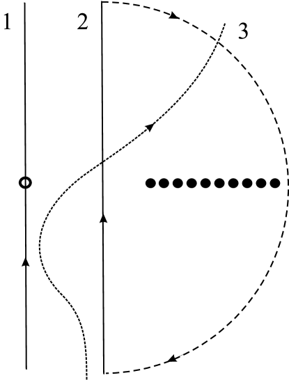
Figure 1: The schematic plot of complex values of $R$ relevant for a single-pair problem. Filled circles show locations of one-electronic levels. Open circle indicates an equilibrium position of $R$ for the ground state. Line 1 shows an integration path through this point in the direction of the steepest descent of $-$Re $W$. Lines 2 and 3 represent examples of integration paths, for which the results of integration will be the same as for the line 1. Dashed line depicts the auxiliary semicircle introduced to use a residue theorem.

For a single-pair problem, $S$ reads as

$$S(R)=\frac{\exp(-R/V)}{\prod_{n=0}^{N_{\Omega}}(2\varepsilon_{F_{0}}+\frac{2n}{\rho}-R)}.$$ (15)

We then perform a partial-fraction decomposition of $1/\prod_{n=0}^{N_{\Omega}}(2\varepsilon_{F_{0}}-R+2n/\rho)$ by using standard rules and rewrite $S$ as

$$S(R)=C\exp(-2\varepsilon_{F_{0}}/V)\sum_{n=0}^{N_{\Omega}}(-1)^{n}\binom{N_{\Omega}}{n}\frac{\exp(-R/V)}{2\varepsilon_{F_{0}}-R+\frac{2n}{\rho}},$$ (16)

where $C$ is an irrelevant $V$-independent constant ($C=\left(\rho/2\right)^{N_{\Omega}}(N_{\Omega}!)^{-1}$), which will be dropped below, as well as similar irrelevant factors, while

$$\binom{N_{\Omega}}{n}=\frac{N_{\Omega}!}{n!(N_{\Omega}-n)!}$$ (17)

is a binomial coefficient. We then substitute Eq. (16) to Eq. (14) and perform an integration. This can be done by various methods. For instance, we may perform integration in a straightforward way, for the integration path along a straight line, like line 2 in Fig. 1. We then see that, of course, the result of the integration depends only on how many poles of function $S$, as given by Eq. (16) (corresponding to the positions of one-electronic levels $2\varepsilon_{\mathbf{k}}$ in the complex plane), is at the right (or left) side of the integration path and it stays the same as long as the number of poles at the right side is the same. In particular, the result is identical for the lines 1 and 2. Alternatively, we can use a residue theorem. For the integration contour, we choose a path, which consists of the line going from $x-iy$ to $x+iy$ (for instance, line 2 in Fig. 1) and then clockwises along a semicircle, as again shown in Fig. 1. We then consider a limit $y\rightarrow\infty$, which ensures that $S$ is infinitely small along the auxiliary semicircle, as follows from Eq. (15). The role of this semicircle is purely technical: it is needed to apply a residue theorem. The result of the integration depends only on how many poles of $S(R)$ are enclosed by the contour. By enclosing the whole set of poles, we arrive to $Z$ corresponding to the ground state of the initial quantum-mechanical problem, for which an equilibrium $R$ is located to the left of the whole set of the one-electronic energies on a complex plane. Enclosing less number of poles leads to $Z$ for excited states, for which an equilibrium $R$ is known to be positioned between two one-electronic levels on real axis (quasi-continuum spectrum). Excited states are beyond the scope of the present paper and will be addressed elsewhere. Note that it is not necessary at all to consider paths consisting of straight lines (see, e.g., curve 3 in Fig. 1).

After integration, we readily obtain a very simple expression for the ground-state $Z$

$$Z=\exp(-2\varepsilon_{F_{0}}/V)\sum_{n=0}^{N_{\Omega}}(-1)^{n}\sigma^{n}\binom{N_{\Omega}}{n}=\exp(-2\varepsilon_{F_{0}}/V)\left(1-\sigma\right)^{N_{\Omega}}.$$ (18)

By finding a logarithmic derivative of $Z$ with respect to $1/V$, we recover a well-known expression of the single-pair energy

$$E_{1}=2\varepsilon_{F_{0}}-2\Omega\frac{\sigma}{1-\sigma},$$ (19)

which also coincides with Eq. (1) for $N=1$.

This method yields the single-pair energy with error of the order of $1/\rho$. The same however applies to the traditional method to derive Eq. (19), which relies on the replacement of the sum by the integral (see Section IV).

The suggested scheme can be applied to the case of many pairs. Let us restrict ourselves for the moment to values of $N$ such that $N\leq N_{\Omega}/2$ for which the degree of the polynomial $\prod_{l,j,j<l}(R_{l}-R_{j})^{2}$ in each $R_{j}$ is smaller than that of the polynomial $\prod_{j=1}^{N}\prod_{\mathbf{k}}(2\varepsilon_{\mathbf{k}}-R_{j})$. It then follows from Eq. (11) that $S(\left\{R_{j}\right\})$, $S(\left\{R_{j}\right\})\sum_{j=1}^{N}R_{j}\rightarrow 0$ at Im $R_{n}\rightarrow\pm\infty$ for any $R_{n}$ from the set $\left\{R_{j}\right\}$.

We consider a system of free charges in the equilibrium and then start to move this system as a whole out of equilibrium, in such a way that mutual distances between free charges stay the same, while the position of the center of mass $\bar{R}$ of this system changes. Now, we concentrate on the change $\delta W$ of $W(\left\{R_{j}\right\})$ upon this motion. By expanding $W(\left\{R_{j}\right\})$ in powers of the deviation $\delta\bar{R}=\bar{R}-\bar{R}^{(0)}$ of $\bar{R}$ from the equilibrium, we easily arrive to the equation

$$\delta W=V\sum_{n=2}^{\infty}\kappa_{n}(\delta\bar{R})^{n},$$ (20)

where

$$\kappa_{n}=-\frac{1}{n}\sum_{j,\mathbf{k}}\frac{1}{(2\varepsilon_{\mathbf{k}}-R_{j}^{(0)})^{n}},$$ (21)

where $R_{j}^{(0)}$ are positions of free charges in equilibrium. Next, we assume that in the ground state all $R_{j}^{(0)}$ are located far enough from the line of fixed charges, so that distances between each free charge and this line are much larger than $1/\rho$. This assumption is rather natural for the thermodynamical limit. Besides, the method for the solution of Richardson equations developed earlier in Ref. [Rich3 ] is also based on the same assumption, since it utilizes a continuous approximation for the positions of free charges. However, in contrast to [Rich3 ], we do not introduce any additional requirements on the shape of a distribution of $R_{j}^{(0)}$ on the complex plane.

In the limit $N\rightarrow\infty$, it follows directly from Eq. (21) that $\kappa_{n}$ depends on system volume as

$$\kappa_{n}\sim\rho N\Omega^{1-n}.$$ (22)

Moreover, $\kappa_{2}$ is purely real due to the mirror symmetry of the system of charges with respect to the real axis. Eq. (22) implies that the absolute value of $S$ is extremely strongly peaked near the equilibrium. Namely, if we go in the direction of the steepest descent of $-$Re $W$, then it is peaked within the interval of the width $\sim 1/\rho$. If we now consider a ratio of integrals similar to the one in Eq. (12), where the integration is performed for the position of the center of mass as well as for internal degrees of freedom of the system of charges, then we can find the equilibrium location of the center of mass, while the error will be in powers in $1/N$, as Eq. (22) suggests, so that it is negligible in the thermodynamical limit. We may formally extend the integration path for $\bar{R}$ from $-i\infty$ to $+i\infty$, where $S$ is zero. At the same time, the integrals entering the ratio are equivalent to the multidimensional integrals with respect to all $R$’s. By using the Cauchy theorem, we may deform the integration path for each $R$, limits of integration being $-i\infty$ and $+i\infty$. Thus, we are led to consider the ratio of integrals defined as in Eq. (12), where an integration is performed for each $R_{j}$. The ratio $E$ will allow us to reconstruct an information about the sum of all $R$’s in an equilibrium, while this is the quantity of interest, since it is equal to the energy of the initial quantum-mechanical system. It is again convenient to introduce $Z$ given by Eq. (14), where an integration is now performed for all variables $R_{j}$ from $-i\infty$ to $+i\infty$. The sum of equilibrium $R$’s is also given by Eq. (13). Eqs. (13) and (14) lead us to associate $Z$ with the ”partition function” for our classical system of charges, although such an analogy is certainly not complete. Nevertheless, we think that this term is far from being meaningless, in the view of Eq. (13). A nontrivial feature is that the energy of the initial quantum mechanical system is determined by the logarithmical derivative of this classical ”partition function”.

Note that our approach has some analogies with thermodynamics. Indeed, for the system of many particles, it is often hopeless to resolve equations for equilibrium positions of each particle. However, such a detailed information is not necessary to understand many global properties of the system, so that a thermodynamical description becomes highly efficient. The major difference with the usual thermodynamics is in the fact that we are dealing with the unstable equilibrium and therefore the ”partition function” is obtained by integrating only over half of the degrees of freedom and by using a complex-valued ”probability”. We also would like to note that the method we here suggest turns out to have similarities with the large-$N$ expansion for the two-dimensional Dyson gas proposed recently in Ref. [Zabrodin ]. Perhaps, our approach may be also related to inverse problems in mathematics. For example, there exists the Radon transform, which allows one to reconstruct an unknown function by using integrals of this function along various paths [Radon ]. This method is widely used in the tomography.

One-dimensional integrals having denominator of the integrand of the form $\prod_{k=0}^{N_{\Omega}}(r-k)$, while integration for $r$ is performed from $-i\infty$ to $+i\infty$ are called Nörlund-Rice integrals. Here we deal with the multidimensional coupled integrals of Nörlund-Rice type. At the same time, factor $\prod_{l,j,j<l}(R_{l}-R_{j})^{2}$ in the integrand makes them similar to Selberg integrals. Note that it is actually known that Nörlund-Rice integrals can be transformed to binomial sums and vise versaSedgewick .

In the next Section, we apply a technique based on binomial sums for finding the ground state energy for arbitrary $N$. However, before doing this, let us address one more point.

We have imposed a restriction $N\leq N_{\Omega}/2$. Configurations with $N\geq N_{\Omega}/2$ can be handled by using a concept of holes, i.e., empty states in the potential layer. In the Appendix A, we show that the initial Hamiltonian is characterized by a duality between electrons and holes, which allows us to map states with $N<N_{\Omega}/2$ to the states with $N>N_{\Omega}/2$.

III Ground state energy through the binomial sum

In this Section, we consider the ground state energy for $N$ pairs, $N\leq N_{\Omega}/2$. It is seen from Eq. (11) that the ”probability” $S$ can be rewritten using a partial-fraction decomposition, in a manner, similar to the one used for the one-pair problem, as

$$S(\left\{R_{j}=2\varepsilon_{F_{0}}-r_{j}\right\})=\exp\left(\frac{-2N\varepsilon_{F_{0}}}{V}\right)\left[\prod_{l,j,l>j}(r_{l}-r_{j})^{2}\right]\sum_{n_{1},n_{2}...,n_{N}=0}^{N_{\Omega}}\left[\prod_{j=1}^{N}(-1)^{n_{j}}\binom{N_{\Omega}}{n_{j}}\frac{\exp(r_{j}/V)}{r_{j}+\frac{2n_{j}}{\rho}}\right].$$ (23)

It can be of interest to note that the sum given by Eq. (23) may be rewritten in terms of the forward difference operators, as usual for binomial sumsumbral ; Sedgewick . This means that Richardson equations can be represented in a similar way too.

After substitution of Eq. (23) to Eq. (14) and integrating in such a way that the integration path for each $R$ avoids the whole set of poles, as for the one-pair problem, we obtain the binomial sum, given by

$$Z=\exp(-2N\varepsilon_{F_{0}}/V)z,$$ (24)

where

$$z=\sum_{n_{1},n_{2}...,n_{N}=0}^{N_{\Omega}}\left[\prod_{j=1}^{N}(-1)^{n_{j}}\sigma^{n_{j}}\binom{N_{\Omega}}{n_{j}}\right]\prod_{l,j,l>j}(n_{l}-n_{j})^{2}.$$ (25)

This sum again corresponds to the ground state of the quantum-mechanical system, for which none of equilibrium $R$’s is located between two one-electronic levels in the real axis.

Without the last factor in the RHS of Eq. (25), this sum reduces to the product of trivial binomial sums for each $n_{j}$, as the one of Eq. (18). In order to tackle the sum with the coupling factor, we first provide some identities, which will be very useful in the derivation presented below.

It is convenient to introduce Pochhammer symbol (or falling factorial) given by

$$(n)_{q}=n(n-1)...(n-q+1),$$ (26)

while $(n)_{0}\equiv 1$. It is then easy to obtain the following identity

$$z_{q,p}\equiv\sum_{n=0}^{N_{\Omega}}(-1)^{n}\sigma^{n}\binom{N_{\Omega}}{n}(n)_{q}(N_{\Omega}-n)_{p}=(-1)^{q}\sigma^{q}(1-\sigma)^{N_{\Omega}-q-p}\frac{N_{\Omega}!}{(N_{\Omega}-q-p)!},$$ (27)

where $q+p\leq N_{\Omega}$. If we now consider a product of sums for each $n_{j}$, every sum being similar to the one of Eq. (27), we get

$$z_{q_{1},p_{1}}...z_{q_{N},p_{N}} = \sum_{n_{1},n_{2}...,n_{N}=0}^{N_{\Omega}}\prod_{j=1}^{N}(-1)^{n_{j}}\sigma^{n_{j}}\binom{N_{\Omega}}{n_{j}}(n_{j})_{q_{j}}(N_{\Omega}-n_{j})_{p_{j}}$$ (28)

$$= \sigma^{\sum_{j=1}^{N}q_{j}}(1-\sigma)^{NN_{\Omega}-\sum_{j=1}^{N}(q_{j}+p_{j})}(-1)^{\sum_{j=1}^{N}q_{j}}\prod_{j=1}^{N}\frac{N_{\Omega}!}{(N_{\Omega}-q_{j}-p_{j})!}.$$

Note that (i) only first two factors in the last line of Eq. (28) depend on the interaction constant $V$ (through $\sigma$); (ii) the dependence of both these factors on the two sets of numbers $\left\{q_{j}\right\}$ and $\left\{p_{j}\right\}$ is only through $\sum_{j=1}^{N}q_{j}$ and $\sum_{j=1}^{N}p_{j}$, which are just degrees of polynomials $\prod_{j=1}^{N}(n_{j})_{q_{j}}$ and $\prod_{j=1}^{N}(N_{\Omega}-n_{j})_{p_{j}}$, respectively. These two observations turn out to be of a crucial importance.

Our approach is to transform the initial coupled sum, as given by Eq. (25), into a linear combination of uncoupled sums, similar to the one given by Eq. (28). To make such an uncoupling, we note that, as known, $\prod_{l,j,l>j}(n_{l}-n_{j})$ can be rewritten as the determinant of the Vandermonde matrix

$$\prod_{l,j,l>j}(n_{l}-n_{j})\equiv V(\left\{n_{j}\right\})=\det\begin{bmatrix}1&1&1&\ldots&1\\ n_{1}&n_{2}&n_{3}&\ldots&n_{N}\\ n_{1}^{2}&n_{2}^{2}&n_{3}^{2}&\ldots&n_{N}^{2}\\ \ldots&\ldots&\ldots&\ldots&\ldots\\ n_{1}^{N-1}&n_{2}^{N-1}&n_{3}^{N-1}&\ldots&n_{N}^{N-1}\end{bmatrix}.$$ (29)

Next step is to note that $\prod_{l,j,l>j}(n_{l}-n_{j})$ can be also written as $(-1)^{N(N-1)/2}V(\left\{N_{\Omega}-n_{j}\right\})$, since $n_{l}-n_{j}=-\left[(N_{\Omega}-n_{l})-(N_{\Omega}-n_{j})\right]$. Hence, we obtain the identity

$$\prod_{l,j,l>j}(n_{l}-n_{j})^{2}=(-1)^{N(N-1)/2}V(\left\{{n_{j}}\right\})V(\left\{N_{\Omega}-n_{j}\right\}).$$ (30)

Now we make use of the well-known rule that the determinant of the matrix does not change if we add a multiple of one row to another row. It is then easy to see that $V(\left\{{n_{j}}\right\})$ can be rewritten in a ”falling factorial” form as

$$V(\left\{{n_{j}}\right\})=\det\begin{bmatrix}(n_{1})_{0}&(n_{2})_{0}&(n_{3})_{0}&\ldots&(n_{N})_{0}\\ (n_{1})_{1}&(n_{2})_{1}&(n_{3})_{1}&\ldots&(n_{N})_{1}\\ (n_{1})_{2}&(n_{2})_{2}&(n_{3})_{2}&\ldots&(n_{N})_{2}\\ \ldots&\ldots&\ldots&\ldots&\ldots\\ (n_{1})_{N-1}&(n_{2})_{N-1}&(n_{3})_{N-1}&\ldots&(n_{N})_{N-1}\end{bmatrix},$$ (31)

while $V(\left\{N_{\Omega}-n_{j}\right\})$ can be represented in a similar form with $n_{j}$ changed into $N_{\Omega}-n_{j}$.

It is obvious that, using Eq. (31), $V(\left\{{n_{j}}\right\})$ can be written as a linear combination of polynomials each having a form $\prod_{j=1}^{N}(n_{j})_{q_{j}}$. The crucial point is that for each term in this sum, $\sum_{j=1}^{N}q_{j}$ is the same: it is just equal to the degree of the polynomial $V(\left\{{n_{j}}\right\})$. This degree is equal to the sum of degrees of polynomials from each row that is to $0+1+...+(N-1)=N(N-1)/2$. The same applies to $V(\left\{N_{\Omega}-n_{j}\right\})$, which is represented as a linear combination of polynomials of the form $\prod_{j=1}^{N}(N_{\Omega}-n_{j})_{p_{j}}$ with $\sum_{j=1}^{N}p_{j}=N(N-1)/2$. Now we see that Eq. (31) together with the similar equation for $V(\left\{N_{\Omega}-n_{j}\right\})$ allows us to rewrite $\prod_{l,j,l>j}(n_{l}-n_{j})^{2}$ as a linear combination of polynomials of the form $\left(\prod_{j=1}^{N}(n_{j})_{q_{j}}\right)\left(\prod_{j=1}^{N}(N_{\Omega}-n_{j})_{p_{j}}\right)$ with the same $\sum_{j=1}^{N}q_{j}$ and $\sum_{j=1}^{N}p_{j}$ for each polynomial. At this stage, we immediately apply Eq. (28) and obtain

$$z=\sigma^{\frac{N(N-1)}{2}}(1-\sigma)^{NN_{\Omega}-N(N-1)}A(N,N_{\Omega}),$$ (32)

where $A(N,N_{\Omega})$ is some function of $N$ and $N_{\Omega}$, which is irrelevant for the determination of the quantum-mechanical energy, since the later is given by the logarithmic derivative of $Z$ with respect to $1/V$. Finally, by finding this logarithmic derivative and by taking into account Eq. (24), we easily arrive to Eq. (1) for the ground state energy.

Eq. (32) can be derived using more formal way of writing. We first note that $V(\left\{{n_{j}}\right\})$ can be expressed in the following form

$$V(\left\{{n_{j}}\right\})\equiv\det(V_{q,p})=\det[(n_{p})_{q-1}]$$

$$=\sum_{j_{1},j_{2},...,j_{N}=1}^{N}\varepsilon_{j_{1}j_{2}...j_{N}}(n_{j_{1}})_{0}(n_{j_{2}})_{1}...(n_{j_{N}})_{N-1},$$ (33)

where $\varepsilon_{j_{1}j_{2}...j_{N}}$ is the Levi-Civita symbol. Similarly, we can write

$$V(\left\{{n_{j}}\right\})V(\left\{N_{\Omega}-{n_{j}}\right\})=\sum_{j_{1},j_{2},...,j_{N}=1}^{N}\varepsilon_{j_{1}j_{2}...j_{N}}\sum_{j_{1}^{\prime},j_{2}^{\prime},...,j_{N}^{\prime}=1}^{N}\varepsilon_{j_{1}^{\prime}j_{2}^{\prime}...j_{N}^{\prime}}$$

$$(n_{j_{1}})_{0}(n_{j_{2}})_{1}...(n_{j_{N}})_{N-1}(N_{\Omega}-n_{j_{1}^{\prime}})_{0}(N_{\Omega}-n_{j_{2}^{\prime}})_{1}...(N_{\Omega}-n_{j_{N}^{\prime}})_{N-1}.$$ (34)

By definition, the Levi-Civita symbol is nonzero only for the set of its indices all different. This means that, for nonzero terms in the double sum in the RHS of Eq. (34), there should be no repetitions in the set $j_{1},j_{2},...,j_{N}$ and also in another set $j_{1}^{\prime},j_{2}^{\prime},...,j_{N}^{\prime}$. We now use Eq. (28) and see that each nonzero term of the double sum gives the same dependence on $V$, when substituted into Eq. (24). Thus, we again arrive to Eq. (32).

In order to reach some qualitative understanding of the result, we have obtained, let us come back to the expression of ”probability”, as given by Eq. (11). We rewrite it as

$$S(\left\{R_{j}=2\varepsilon_{F_{0}}-r_{j}\right\}) = \exp(-2N\varepsilon_{F_{0}}/V)\frac{1}{\prod_{j=1}^{N}\prod_{n=0}^{\rho\Omega}(r_{j}+\frac{2n}{\rho})}\exp\left(\frac{\sum_{j=1}^{N}r_{j}}{V}\right)$$ (35)

$$\det\begin{bmatrix}1&1&\ldots&1\\ \prod_{n=0}^{0}(r_{1}+\frac{2n}{\rho})&\prod_{n=0}^{0}(r_{2}+\frac{2n}{\rho})&\ldots&\prod_{n=0}^{0}(r_{N}+\frac{2n}{\rho})\\ \ldots&\ldots&\ldots&\ldots\\ \prod_{n=0}^{N-2}(r_{1}+\frac{2n}{\rho})&\prod_{n=0}^{N-2}(r_{2}+\frac{2n}{\rho})&\ldots&\prod_{n=0}^{N-2}(r_{N}+\frac{2n}{\rho})\end{bmatrix}$$

$$\det\begin{bmatrix}1&1&\ldots&1\\ \prod_{n=0}^{0}(r_{1}+2\Omega-\frac{2n}{\rho})&\prod_{n=0}^{0}(r_{2}+2\Omega-\frac{2n}{\rho})&\ldots&\prod_{n=0}^{0}(r_{N}+2\Omega-\frac{2n}{\rho})\\ \ldots&\ldots&\ldots&\ldots\\ \prod_{n=0}^{N-2}(r_{1}+2\Omega-\frac{2n}{\rho})&\prod_{n=0}^{N-2}(r_{2}+2\Omega-\frac{2n}{\rho})&\ldots&\prod_{n=0}^{N-2}(r_{N}+2\Omega-\frac{2n}{\rho})\end{bmatrix}.$$

It is seen from the above equation that the ”probability” $S(\left\{R_{j}\right\})$ can be represented in a factorized form as a sum of products of $N$ ”probabilities”, each of them being the one for a single pair. Each single pair is however placed into its own environment with a band of one-electronic states removed from the bottom of the potential layer and another band of states removed from the top of the potential layer, as a result of the Pauli exclusion principle. The energy of a single pair in the state with $n$ levels removed from the bottom of the potential layer and $m$ states removed from the top of the layer is obtained from Eq. (19) by substitution $\varepsilon_{F_{0}}\rightarrow\varepsilon_{F_{0}}+n/\rho$, $\Omega\rightarrow\Omega-(n+m)/\rho$. Hence, it follows from Eq. (35) that the sum of single-pair energies is the same for each term of the factorized ”probability”, although sets of single-pair energies for different terms are not identical.

We therefore can think that the original system of $N$ pairs, feeling each other through the Pauli exclusion principle, is a superposition of ”states” of $N$ single pairs, but each pair is placed into its own environment with bands of the states deleted both from the bottom and from the top of the potential layer. Moreover, the sum of energies of these single pairs for each ”state” of the superposition is the same, which is, probably, a consequence of the constant density of states. This understanding provides an additional nontrivial link between the one-pair problem, solved by Cooper, and many-pair BCS theory.

Note that we see here a quite close analogy with the well-known Hubbard-Stratonovich transformation [Strat ; Hub ], which enables one to represent the partition function for the system of interacting particles through the partition function for the system of noninteracting (single) particles, but in the fluctuating field. We also would like to mention that some of the ”probabilities” appearing in Eq. (35) can be negative; one should not be confused by this fact, since negative ”probabilities” are known to appear in problems involving fermions. In particular, they lead to the well-known negative sign problem arising when trying to apply Monte Carlo methods to compute partition functions. This problem becomes severe in the thermodynamical limit. Actually, we here see some reminiscence of the same problem. Namely, if we try to integrate factorized $S$ through paths crossing individual saddle points of each single pair, we immediately see that the absolute value of resulting $Z$ is going to be much smaller than the result of the integration for each term due to the ”determinantal” structure of Eq. (35). The easiest way to see it is to consider the two-pair problem. The situation is getting more and more difficult with the increase of $N$. Fortunately, by applying the method based on binomial sums, we can circumvent all these difficulties and to evaluate $Z$ exactly.

IV Ground state energy through the Nörlund-Rice integral

In this Section, we present another method, which allows us to find the ground state energy as an expansion in powers of pairs density. In practise, this method is much less powerful compared to the one described in the previous Section. We here calculate just few first terms of the expansion, since calculations become more and more heavy with increasing number of terms. One of the main aims of this Section is actually to establish a link between our approach and the dilute-limit approach of Refs. [We ; EPJB ]. The method presented in this Section turns out to be closely related to the method of Refs. [We ; EPJB ].

The general idea is not to transform the initial multidimensional integral of Nörlund-Rice type into a binomial sum, but to tackle it by using a saddle-point method. For $z$, we have

$$z=\int dr\frac{\prod_{l,j,j<l}(r_{l}-r_{j})^{2}}{\prod_{j=1}^{N}\prod_{m_{j}=0}^{N_{\Omega}}(r_{j}+\frac{2m_{j}}{\rho})}\exp\left(\frac{\sum_{j=1}^{N}r_{j}}{V}\right),$$ (36)

where

$$\int dr=\int dr_{1}\ldots\int dr_{N}.$$

Quantum-mechanical energy $E$ is expressed through the logarithmic derivative of $z$ with respect to $1/V$ as

$$E\equiv 2N\varepsilon_{F_{0}}-\frac{\partial ln(z)}{\partial(1/V)}=2N\varepsilon_{F_{0}}-\frac{1}{z}\int dr\left(\sum_{j=1}^{N}r_{j}\right)\frac{\prod_{l,j,j<l}(r_{l}-r_{j})^{2}}{\prod_{j=1}^{N}\prod_{m_{j}=0}^{N_{\Omega}}(r_{j}+\frac{2m_{j}}{\rho})}\exp\left(\frac{\sum_{j=1}^{N}r_{j}}{V}\right)$$ (37)

The factor $\prod_{l,j,j<l}(r_{l}-r_{j})^{2}$ is responsible for the coupling between $r_{j}$’s. In order to see the effect of this coupling, we use the path of integration for each $r_{j}$, which passes through the stationary point corresponding to a single pair (line 1 in Fig. 1). This point yields the one-pair energy, as found by Cooper.

Because of the symmetry between all $r_{j}$’s in the RHS of Eq. (37), we may replace $\sum_{j=1}^{N}r_{j}$ by $Nr_{1}$. Then, $E$ can be rewritten as

$$E=2N\varepsilon_{F_{0}}-N\frac{F_{1}}{F_{0}},$$ (38)

where

$$F_{n} \equiv \int drr_{1}^{n}\frac{\prod_{l,j,j<l}(r_{l}-r_{j})^{2}}{\prod_{j=1}^{N}\prod_{m_{j}=0}^{N_{\Omega}}(r_{j}+\frac{2m_{j}}{\rho})}\exp\left(\frac{\sum_{j=1}^{N}r_{j}}{V}\right)$$ (39)

$$= \int drr_{1}^{n}\left[\prod_{j=1}^{N}\exp\left(\frac{r_{j}}{V}-\sum_{m_{j}=0}^{N_{\Omega}}\ln\left(r_{j}+\frac{2m_{j}}{\rho}\right)\right)\right]\prod_{l,j,j<l}(r_{l}-r_{j})^{2}.$$

The position of the saddle point is given by the solution of the following equation:

$$\frac{\partial}{\partial r}f(r)\equiv\frac{\partial}{\partial r}\left[\frac{r}{V}-\sum_{m=0}^{N_{\Omega}}\ln\left(r+\frac{2m}{\rho}\right)\right]=\frac{1}{V}-\sum_{m=0}^{N_{\Omega}}\frac{1}{r+\frac{2m}{\rho}}=0.$$ (40)

We replace sum by the integral that is justified in the large-sample limit, and find the solution of Eq. (40), $r=\epsilon_{c}$, which gives the binding energy of an isolated Cooper pair

$$\epsilon_{c}\simeq 2\Omega\frac{\sigma}{1-\sigma},$$ (41)

which actually has already been found in Eq. (19) through the binomial sum. We now introduce a new variable $t$ defined as $it=r-\epsilon_{c}$. Next, we expand $f(r)$ in a Taylor series around $r=\epsilon_{c}$ and rewrite it as

$$f(\epsilon_{c}+it)=f(\epsilon_{c})+\varphi(t),$$ (42)

where $\varphi(t)$ reads as

$$\varphi(t)=\sum_{m=2}^{+\infty}\frac{f^{(m)}(\epsilon_{c})}{m!}(it)^{m}.$$ (43)

Derivatives $f^{(m)}(\epsilon_{c})$ can be easily found from Eqs. (40) and (41) as

$$f^{(m)}(\epsilon_{c})\simeq(-1)^{m}(m-2)!\frac{\rho}{2}\left(\frac{1-\sigma}{2\Omega\sigma}\right)^{m-1}(1-\sigma^{m-1}).$$ (44)

Notice that we again have replaced sums by integrals, when deriving Eq. (44).

It is seen from Eq. (44) that $f^{(2)}(\epsilon_{c})$ is positive, since $\sigma<1$. Thus, the direction of the steepest descent for $\exp(f(r))$ is perpendicular to the real axis in $r$ complex plane, as expected (line 1 in Fig. 1). Hence, we assume that $t$ changes from $-\infty$ to $+\infty$. Next, we introduce a rescaled variable $x$ instead of $t$

$$x=t\sqrt{f^{(2)}(\epsilon_{c})}.$$ (45)

Within new notations, $f$ reads as

$$f\left(\epsilon_{c}+ix/\sqrt{f^{2}(\epsilon_{c})}\right)=f(\epsilon_{c})+\sum_{m=2}^{\infty}\alpha_{m}x^{m},$$ (46)

where

$$\alpha_{m}=\frac{(-i)^{m}}{m(m-1)}\frac{1-\sigma^{m-1}}{1-\sigma}\delta^{m-2},$$ (47)

where $\delta$ is a small dimensionless constant which is inversely proportional to the square root of the system volume

$$\delta=\frac{1}{\sqrt{\rho\Omega\sigma}}.$$ (48)

Note that $\alpha_{2}=-1/2$.

The existence of the small constant $\delta$ is crucial in our derivation, since we are going to calculate the ground state energy as an asymptotic expansion in powers of $\delta$. We will however see that $\delta$ is going to be coupled with the number of pairs, so the resulting expansion of the energy density in the thermodynamical limit will be in powers of pair density, which is proportional to $N\delta^{2}\sim N/\rho$ and is no longer small. Such an unusual feature is due to the fact that we here deal with the multidimensional integral, while integration is performed through the single-pair saddle point.

Next, we rewrite Eq. (38) as

$$E=2N\varepsilon_{F_{0}}-N\epsilon_{c}-iN\delta\frac{2\Omega\sigma}{1-\sigma}\frac{\Phi_{1}}{\Phi_{0}},$$ (49)

where

$$\Phi_{n}=\int dxx_{1}^{n}\left[\prod_{j=1}^{N}\exp\left(\sum_{m=2}^{\infty}\alpha_{m}x_{j}^{m}\right)\right]\prod_{l,j,j<l}(x_{l}-x_{j})^{2},$$ (50)

where integration for each $x_{j}$ is performed from $-\infty$ to $+\infty$.

Let us concentrate on $\Phi_{1}$. It can be integrated by parts with respect to $x_{1}$ in the following manner:

$$\Phi_{1}=\int dx\left[\prod_{j,l,j<l}(x_{l}-x_{j})^{2}e^{\sum_{m=3}^{\infty}\alpha_{m}x_{1}^{m}}\right]_{x_{1}}^{\prime}e^{\alpha_{2}x_{1}^{2}}\prod_{j\neq 1}e^{\sum_{m=2}^{\infty}\alpha_{m}x_{j}^{m}}.$$ (51)

The derivative in the integrand in the RHS of the above equation reads

$$2\sum_{j_{1}\neq 1}(x_{1}-x_{j_{1}})\prod_{\begin{subarray}{c}l,j,j<l,\\ (j,l)\neq(1,j_{1})\end{subarray}}(x_{l}-x_{j})^{2}e^{\sum_{m=3}^{\infty}\alpha_{m}x_{1}^{m}}$$

$$+\delta\sum_{m=2}^{\infty}a_{m}\delta^{m-2}x_{1}^{m}\left[\prod_{l,j,j<l}(x_{l}-x_{j})^{2}e^{\sum_{m=3}^{\infty}\alpha_{m}x_{1}^{m}}\right],$$ (52)

where

$$a_{m}=\alpha_{m+1}(m+1)\delta^{-(m-1)}=\frac{(-i)^{m+1}}{m}\frac{1-\sigma^{m}}{1-\sigma}.$$ (53)

The first term in Eq. (52) vanishes identically after we substitute it into Eq. (51) and perform integration over all $x_{j}$’s, due to the symmetry reasons, which can be easily verified upon the mutual exchange $x_{1}\longleftrightarrow x_{j_{1}}$. The second term, after the integration, yields an expansion of $\Phi_{1}$ through $\Phi_{2}$, $\Phi_{3}$, etc. with coefficients, which represent higher and higher powers of $\delta$

$$\Phi_{1}=\delta\sum_{m=2}^{\infty}a_{m}\delta^{m-2}\Phi_{m}.$$ (54)

We now focus on the first term in the expansion from the RHS of Eq. (54), which is linear in $\delta$. $\Phi_{2}$ can be handled in the same manner, as the one used for $\Phi_{1}$. Namely, we make integration by parts with respect to $x_{1}$. We then obtain an equation, similar to Eq. (51), except that the expression in square brackets must be multiplied by $x_{1}$. The derivative of this expression can be written as

$$\prod_{l,j,j<l}(x_{l}-x_{j})^{2}e^{\sum_{m=3}^{\infty}\alpha_{m}x_{1}^{m}}$$

$$+2x_{1}\sum_{j_{1}\neq 1}(x_{1}-x_{j_{1}})\prod_{\begin{subarray}{c}l,j,j<l,\\ (j,l)\neq(1,j_{1})\end{subarray}}(x_{l}-x_{j})^{2}e^{\sum_{m=3}^{\infty}\alpha_{m}x_{1}^{m}}$$

$$+\delta\sum_{m=2}^{\infty}a_{m}\delta^{m-2}x_{1}^{m+1}\prod_{l,j,j<l}(x_{l}-x_{j})^{2}e^{\sum_{m=3}^{\infty}\alpha_{m}x_{1}^{m}}.$$ (55)

After integration, the first term in the RHS of the above equation gives $\Phi_{0}$. The second term is the sum of $N-1$ terms. By performing a mutual exchange $x_{1}\longleftrightarrow x_{j_{1}}$, it is easy to see that each of these terms also gives $\Phi_{0}$ after the integration. The third term leads to the linear combination of $\Phi_{m}$’s with $m$ starting from $3$. As a result, $\Phi_{2}$ reads

$$\Phi_{2}=N\Phi_{0}+\delta\sum_{m=2}^{\infty}a_{m}\delta^{m-2}\Phi_{m+1}.$$ (56)

At this stage, we substitute Eq. (56) to the expression of $\Phi_{1}$, as given by Eq. (54), and obtain

$$\Phi_{1} = \delta N\Phi_{0}a_{2}+\delta^{2}\sum_{m=2}^{\infty}a_{m+1}^{(1)}\delta^{m-2}\Phi_{m+1}$$ (57)

$$= \delta N\Phi_{0}a_{2}+O(\delta^{2}),$$

where $a_{m+1}^{(1)}$ is a ”new” expansion coefficient, given by

$$a_{m+1}^{(1)}=a_{m+1}+a_{2}a_{m}.$$ (58)

Eq. (57) provides $\Phi_{1}/\Phi_{0}$ in lowest order in $\delta$. It is then substituted to the expression for the energy, given by Eq. (49). Together with Eq. (53) for $m=2$ and the definition of $\delta$ it leads to

$$E=E_{N}+\frac{N}{\rho}\frac{1+\sigma}{1-\sigma}+O\left(\rho^{-3/2}\right),$$ (59)

where $E_{N}$ is given by Eq. (1). The second term in the RHS of Eq. (59) is underextensive, so that it can be dropped. Of course, one has to keep in mind that the third term, $O\left(\rho^{-3/2}\right)$, is not necessarily small due to the coupling with $N$.

Thus, we have calculated the correction to the energy of $N$ noninteracting pairs in the lowest order in $\delta$, which gives nonzero contribution, i.e., in $\delta^{2}$. This correction turns out to be proportional to $N(N\delta^{2})$ (due to the coupling with $N$) that is extensive. Moreover, this first correction already gives the total energy within all relevant (extensive) terms, as evident from the results of Section III. The task is now to prove that the third term in the RHS of Eq. (59), produces underextensive contribution only. This problem is addressed in the Appendix B, where we show, through rather tedious calculations, that two next terms in $\delta$ are indeed underextensive. We stress that we are unable to present a complete proof involving all terms of the expansion. The underextensivity we have revealed follows from ”magic rules” for coefficients $a_{m}$, which are of course linked to the constant density of states. Thus, the method based on calculation of the binomial sum, which enabled us to derive the expression for the ground state energy directly within all extensive terms in a simple way (nonperturbatively in $\delta$), appears to be much more efficient than the method of the present Section.

We also wish to stress that the method of saddle-point evaluation of Nörlund-Rice integral through the single-pair solution is quite similar to the method of analytical solution of Richardson equations presented in Ref. [We ] and advanced further in Ref. [EPJB ]. In Ref. [We ], all Richardson energy-like quantities $R$’s have been expanded around a single-pair solution in seria involving small dimensionless parameter analogous to $\delta$. By keeping only the lowest-order contribution, Eq. (1) has been derived. The lowest-order approximation a priori makes this method restricted to the dilute regime of pairs only, when their density is small. However, in Ref. [EPJB ] it was demonstrated that next term in the small dimensionless parameter vanishes identically due to the first ”magic cancellation”, which implies that the dilute-limit result of Ref. [ We ] is likely to be universal. We have arrived to the similar conclusion within our framework, but we have also revealed the second ”magic cancellation” which exists for the next-order term (see the Appendix B).

The method of integration through the single-pair saddle point, as presented in this Section, has some disadvantages (in addition to its obvious technical complexity compared to the method based on manipulations with binomial sums). Namely, it relies on replacing sums by integrals, as we did to derive Eq. (41). More rigorously, sums of this kind should be expressed through $\Gamma$-functions. By keeping a leading order term in the expansion of these $\Gamma$-functions in $1/\rho$, one obtains the approximation, used here. Dropping all the remaining terms introduces errors of the order of $\delta^{2}\sim 1/\rho$ in many places. Fortunately, this approximation does not lead to any pathologies for extensive quantities, but it produces artificial underextensive terms (not considered here). In addition, the effect of the reduction of a pair binding energy in a many-pair configurationWe compared to the isolated pair is clearly of discrete origin, while, within this approach, it is recovered through the continuous approximation, i.e., in a very indirect way.

V Conclusions

Within the exact mapping of Richardson equations to the system of interacting charges in the plane, we suggested to switch from the ”energy” of this system to the ”probability” for charges to occupy certain states in configurational space at the effective temperature given by the interaction constant. The effective temperature thus goes to zero when system volume goes to infinity. We introduced a ”partition function”, from which the ground state energy of the initial quantum-mechanical many-body problem can be found. This approach leads to the emergency of quite rich mathematical structure. The ”partition function” has a form of a multidimensional integral, similar to Selberg integrals. For the model with constant density of energy states, the structure of the integrand implies that it can be also considered as an integral of Nörlund-Rice type. The most efficient way to evaluate it is by transforming the integral into a binomial sum, where the coupling between variables is due to the determinant of the Vandermonde matrix. Using properties of this matrix, we managed to evaluate the ”partition function” exactly in a rather simple way and to find the ground state energy, which is described by a single expression all over from the dilute to the dense regime of pairs. This expression does coincides with the mean-field BCS result.

We also provided a qualitative understanding of the obtained result in terms of ”probabilities”. Namely, the ”probability” of the system of $N$ pairs, feeling each other through the Pauli exclusion principle, to be in a certain state can be represented in a factorized form as a linear combination of terms. Each of them is given by the product of ”probabilities” for $N$ single pairs, but every single pair is placed into its own environment, which is identical to the initial one, except that two bands of the one-electronic energy states - both from the bottom and from the top of energy interval - are absent due to the Pauli exclusion principle. Moreover, we find that although these environments are different, the sum of energies of the single pairs is the same for all terms of factorized ”probability”.

Finally, we presented another method for evaluation of the Nörlund-Rice integral by integration through the saddle point corresponding to a single pair. This method turns out to be much less efficient; it exactly corresponds to the dilute-limit approach for the solution of Richardson equation proposed very recently in Refs. We ; EPJB . Nevertheless, we managed to calculate several initial terms of the expansion of energy in pairs density.

The suggested method is rather general and we believe that it can be applied to other integrable pairing Hamiltonians, which have electrostatic analogiesAmico ; Ibanez , as well as to situations with nonconstant density of energy states.

Appendix A Electrons-holes duality

We introduce creation operators for holes as $b_{\mathbf{k}\uparrow}^{\dagger}=a_{\mathbf{k}\uparrow}$ and $b_{\mathbf{k}\downarrow}^{\dagger}=a_{\mathbf{k}\downarrow}$ with corresponding rules for destruction operators. These holes should not be confused with holes in the Fermi sea of normal electrons, as appear in BCS theory. By using commutation relations for fermionic operators, it is rather easy to rewrite the initial Hamiltonian in terms of holes as

$$H=-V\sum_{\mathbf{k}}1+2\sum_{\mathbf{k}}\varepsilon_{\mathbf{k}}-\sum_{\mathbf{k}}\left(\varepsilon_{\mathbf{k}}-V\right)\left(b_{\mathbf{k}\uparrow}^{\dagger}b_{\mathbf{k}\uparrow}+b_{\mathbf{k}\downarrow}^{\dagger}b_{\mathbf{k}\downarrow}\right)-V\sum_{\mathbf{k},\mathbf{k}^{\prime}}b_{\mathbf{k}^{\prime}\uparrow}^{\dagger}b_{-\mathbf{k}^{\prime}\downarrow}^{\dagger}b_{-\mathbf{k}\downarrow}b_{\mathbf{k}\uparrow}.$$ (60)

The first two terms of the RHS of Eq. (60) are scalars. Moreover, the first term, $V\sum_{\mathbf{k}}1$, is inderextensive and can be dropped. The fourth term in the RHS of Eq. (60) is fully identical to the interaction potential in terms of electrons, given by Eq. (2). To better understand the role of the third term, we introduce $\xi_{\mathbf{k}}^{{}^{\prime}}$ defined as $\xi_{\mathbf{k}}^{{}^{\prime}}=$ $\varepsilon_{F_{0}}+\Omega-\varepsilon_{\mathbf{k}}$. In the case of a constant density of states, $\xi_{\mathbf{k}}^{{}^{\prime}}$ is $0$, $1/\rho$, $2/\rho$, …, $\Omega$: $\xi_{\mathbf{k}}^{{}^{\prime}}$ just counts states starting from the top of potential layer towards its bottom. Hence, $-(\varepsilon_{\mathbf{k}}-V$) can be rewritten as $\xi_{\mathbf{k}}^{{}^{\prime}}-(\varepsilon_{F_{0}}+\Omega-V)$. A similar term in the Hamiltonian for electrons, given by Eq. (3), contains factor $\xi_{\mathbf{k}}+\varepsilon_{F_{0}}$. Thus, we clearly see a duality between electrons and holes: The ground state of $N$ pairs is equivalent to the ground state of $N_{\Omega}-N$ holes, while the energy of the latter is equal to the energy of $N_{\Omega}-N$ pairs, with $\varepsilon_{F_{0}}$ changed into $-(\varepsilon_{F_{0}}+\Omega-V)$, plus the kinetic energy of the potential layer completely filled, given by $2\sum_{\mathbf{k}}\varepsilon_{\mathbf{k}}$. This means that we can avoid considering configurations with $N>N_{\Omega}/2$ by switching to holes, Cooper pairs in this case being constructed out of them. Moreover, one can directly check that the expression of the ground state energy given by Eq. (1), which we are going to prove, satisfies, within underextensive terms, the above duality criterion. Therefore, it is sufficient to consider the case $N<N_{\Omega}/2$ only. The existence of the duality between electrons and holes in the energy spectrum has already been noted in Ref. [We ; MWO ], although its origin, at the level of the Hamiltonian, stayed unclear.

Appendix B Cancellation of higher-order terms in pairs density

We focus on $\Phi_{3}$ and rewrite it through the integration by parts, as has been done for $\Phi_{1}$ and $\Phi_{2}$

$$\Phi_{3}=2N\Phi_{1}+\delta\sum_{m=2}^{\infty}a_{m}\delta^{m-2}\Phi_{m+2}.$$ (61)

Next, we substitute Eq. (61) to the first line of Eq. (57) and get the following expression of $\Phi_{1}/\Phi_{0}$

$$\frac{\Phi_{1}}{\Phi_{0}}=\delta Na_{2}\frac{1}{1-2\delta^{2}Na_{3}^{(1)}}\left(1+\frac{\delta^{2}}{Na_{2}}\sum_{m=3}^{\infty}a_{m+1}^{(2)}\delta^{m-3}\frac{\Phi_{m+1}}{\Phi_{0}}\right),$$ (62)

where

$$a_{m+1}^{(2)}=a_{m+1}^{(1)}+a_{3}^{(1)}a_{m-1}.$$ (63)

We now consider the first term of the sum in the RHS of Eq. (62). Again integrating by parts, we obtain

$$\Phi_{4}\simeq 2N\Phi_{2}+N\Phi_{1,1}+\delta\sum_{m=4}^{\infty}a_{m-2}\delta^{m-4}\Phi_{m+1},$$ (64)

while $\Phi_{m,n}$ is given by Eq. (50) with $x_{1}^{n}$ replaced by $x_{1}^{m}x_{2}^{n}$. $\Phi_{1,1}$ is evaluated as

$$\Phi_{1,1}=-\Phi_{0}+\delta\sum_{m=1}^{\infty}a_{m+1}\delta^{m-1}\Phi_{1,m+1}.$$ (65)

Now we substitute Eq. (65) for $\Phi_{1,1}$ and Eq. (56) for $\Phi_{2}$ to Eq. (64) for $\Phi_{4}$, and the resulting equation for $\Phi_{4}$ - to Eq. (62) for $\Phi_{1}$. The obtained expression of $\Phi_{1}$ can be written as a sum of two contributions

$$\Phi_{1}=G_{1}+G_{2},$$ (66)

where

$$G_{1}=\delta N\frac{\Phi_{0}a_{2}}{1-2a_{3}^{(1)}\delta^{2}N}\left(1+\frac{2a_{4}^{(2)}}{a_{2}}\delta^{2}N\right),$$ (67)

$$G_{2}=\frac{\delta^{4}}{1-2a_{3}^{(1)}\delta^{2}N}\left(\sum_{m=4}^{\infty}a_{m+1}^{(3)}\delta^{m-4}\Phi_{m+1}+a_{4}^{(2)}N\sum_{m=2}^{\infty}a_{m}\delta^{m-2}(2\Phi_{m+1}+\Phi_{1,m})\right),$$ (68)

where

$$a_{m+1}^{(3)}=a_{m+1}^{(2)}+a_{4}^{(2)}a_{m-2}.$$ (69)

It is can be checked that

$$a_{4}^{(2)}+a_{3}^{(1)}a_{2}=0$$ (70)

for any $\sigma$. Therefore, due to the exact cancellation between the numerator and denominator, Eq. (67) for $G_{1}$ is reduced to

$$G_{1}=(\delta N)\Phi_{0}a_{2}.$$ (71)

This means that terms proportional to $N\delta(N\delta^{2})=N^{2}\delta^{3}$, which are present in $G_{1}$ and not in $G_{2}$, are absent in the expansion of $\Phi_{1}/\Phi_{0}$ in powers of $\delta$. As clearly seen from Eq. (49), these are exactly the terms, which give contribution of the order of $N(N/\rho)^{2}\sim N(N\delta^{2})^{2}$ to the energy, or equivalently, terms in square of pairs density ($\sim(N/\rho)^{2}$) to the energy density. Eq. (70) constitutes first ”magic cancellation” rule and it is fully equivalent to Eq. (68) of Ref. [EPJB ].

Let us now make some comments. In general, at each step of our procedure, we express $\Phi_{m}$ through the linear combination of all possible terms of the form $\Phi_{m_{1},m_{2},...}$, with the sum of nonnegative integer $m$’s equal to $m-2$ and prefactors, independent on $\delta$, plus expansion which involves $\delta^{n}\Phi_{m+n}$, $n$ starting from 1. We then have to proceed with all these ”new” $\Phi_{m_{1},m_{2},...}$’s to lower the sum of $m$’s by 2 at each iteration and finally to bring them either to $\Phi_{0}$ or to $\Phi_{1}$, depending on a parity of $m$. And so on. Of course, this recursive tree-like procedure becomes more and more tedious when $m$ is increasing. That is why we were able to trace only few first terms of the expansion.

Now we provide a sketch for the derivation of the next-order correction to the energy, which will be of the order of $N(N/\rho)^{3}$. For that, we first have to consider $\Phi_{5}$. We express $\Phi_{5}$ through $\Phi_{3}$ (given by Eq. (61)), $\Phi_{1,2}$, and $\Phi_{n}$ for $n$’s starting from $6$. $\Phi_{1,2}$ is expressed through $\Phi_{1}$ and $\Phi_{2,n}$, with $n$ starting from 2. Then, we perform similar manipulations for $\Phi_{6}$. Next, we substitute all these quantities to Eqs. (66)-(68) for $\Phi_{1}$ and obtain more sophisticated fraction than the one in the RHS of Eq. (62) which now includes higher powers of $\delta$.

By expanding this ”new” fraction in $\delta$, we finally ensure that terms of $\Phi_{1}/\Phi_{0}$ in $N\delta(N\delta^{2})^{2}=N^{3}\delta^{5}$ vanish due to the second ”magic cancellation” rule, given by

$$5a_{6}^{(4)}+10a_{5}^{(3)}a_{2}+a_{4}^{(2)}(4a_{3}+9a_{2}^{2})=0,$$ (72)

where

$$a_{m+1}^{(4)}=a_{m+1}^{(3)}+a_{5}^{(3)}a_{m-3}.$$ (73)

Again, Eq. (72) is fulfilled for any $\sigma$. Then, it follows from Eq. (49) that terms in $N(N/\rho)^{3}\sim N(N\delta^{2})^{3}$ vanish in the expression of the quantum-mechanical energy.